Non Local Spatial and Angular Matching :
Enabling higher spatial resolution diffusion MRI datasets through adaptive denoising

Abstract

Diffusion magnetic resonance imaging (MRI) datasets suffer from low Signal-to-Noise Ratio (SNR), especially at high b-values. Acquiring data at high b-values contains relevant information and is now of great interest for microstructural and connectomics studies. High noise levels bias the measurements due to the non-Gaussian nature of the noise, which in turn can lead to a false and biased estimation of the diffusion parameters. Additionally, the usage of in-plane acceleration techniques during the acquisition leads to a spatially varying noise distribution, which depends on the parallel acceleration method implemented on the scanner. This paper proposes a novel diffusion MRI denoising technique that can be used on all existing data, without adding to the scanning time. We first apply a statistical framework to convert both stationary and non stationary Rician and non central Chi distributed noise to Gaussian distributed noise, effectively removing the bias. We then introduce a spatially and angular adaptive denoising technique, the Non Local Spatial and Angular Matching (NLSAM) algorithm. Each volume is first decomposed in small 4D overlapping patches, thus capturing the spatial and angular structure of the diffusion data, and a dictionary of atoms is learned on those patches. A local sparse decomposition is then found by bounding the reconstruction error with the local noise variance. We compare against three other state-of-the-art denoising methods and show quantitative local and connectivity results on a synthetic phantom and on an in-vivo high resolution dataset. Overall, our method restores perceptual information, removes the noise bias in common diffusion metrics, restores the extracted peaks coherence and improves reproducibility of tractography on the synthetic dataset. On the 1.2 mm high resolution in-vivo dataset, our denoising improves the visual quality of the data and reduces the number of spurious tracts when compared to the noisy acquisition. Our work paves the way for higher spatial resolution acquisition of diffusion MRI datasets, which could in turn reveal new anatomical details that are not discernible at the spatial resolution currently used by the diffusion MRI community.

1 Introduction

Diffusion magnetic resonance imaging (MRI) is an imaging technique that allows probing microstructural features of the white matter architecture of the brain. Due to the imaging sequence used, the acquired images have an inherently low signal-to-noise ratio (SNR), especially at high b-values. Acquiring data at high b-values contains relevant information and is now of great interest for connectomics (Van Essen et al., 2013) and microstructure (Alexander et al., 2010) studies. High noise levels bias the measurements because of the non-Gaussian nature of the noise, which in turn prohibits high resolution acquisition if no further processing is done. This can also lead to a false and biased estimation of the diffusion parameters, which impacts on the scalar metrics (e.g. fractional anisotropy (FA)), or in the fitting of various diffusion models (e.g. diffusion tensor imaging (DTI) and high angular resolution diffusion imaging (HARDI) models). This can further impact subsequent tractography and connectivity analysis if the spatially variable noise bias is not taken into account. Therefore, high SNR diffusion weighted images (DWIs) are crucial in order to draw meaningful conclusions in subsequent data or group analyses (Jones et al., 2013).

This paper focuses on denoising techniques since they can be used on all existing data, without adding to the scanning time. They also can be readily applied to any already acquired dataset just like motion and eddy current corrections that are commonly applied on acquired datasets. One possible way to acquire higher quality data is to use better hardware, but this is costly and not realistic in a clinical setting. One can also use a bigger voxel size in order to keep the relative SNR at the same level, but at the expense of a lower spatial resolution or acquiring fewer directions to keep an acceptable acquisition time (Descoteaux and Poupon, 2014). Averaging multiple acquisitions also increases the SNR, but this should be done either using Gaussian distributed noisy data (Eichner et al., 2015) or in the complex domain to avoid the increased noise bias (Jones et al., 2013).

With the advance of parallel imaging and acceleration techniques such as the generalized autocalibrating partially parallel acquisitions (GRAPPA) or the sensitivity encoding for fast MRI (SENSE), taking into account the modified noise distribution is the next step (Dietrich et al., 2008; Aja-Fernández et al., 2014). The noise is usually modeled with a Rician distribution when SENSE is used and a non central Chi (nc-$\chi$) distribution with 2N degrees of freedom (with N the number of receiver coils) when a Sum of Squares (SoS) reconstruction is used. If GRAPPA acceleration is also used with a SoS reconstruction, the degrees of freedom of the nc-$\chi$ distribution will vary between 1 and 2N (Aja-Fernández et al., 2014). Some techniques have been specifically adapted by the medical imaging community to take into account the Rician nature of the noise such as non local means algorithms (Tristán-Vega and Aja-Fernández, 2010; Coupé et al., 2008; Manjón et al., 2010), Linear Minimum Mean Square Error estimator (Aja-Fernandez et al., 2008; Brion et al., 2013), generalized total variation (Liu et al., 2014), a majorize-minimize framework with total variation denoising (Varadarajan and Haldar, 2015), maximum likelihood (Rajan et al., 2012) or block matching (Maggioni et al., 2013). Some methods  (Tristán-Vega and Aja-Fernández, 2010; Brion et al., 2013; Manjón et al., 2013; St-Jean et al., 2014; Bao et al., 2013; Becker et al., 2014; Gramfort et al., 2014; Lam et al., 2014) have also been specifically designed to take advantage of the properties of the diffusion MRI signal such as symmetry, positivity or angular redundancy. Since the data acquired in diffusion MRI depicts the same structural information, but under different sensitizing gradients and noise realization, these ideas take advantage of the information contained in the multiple acquired diffusion MRI datasets.

We thus propose to exploit the structural redundancy across DWIs through a common sparse representation using dictionary learning and sparse coding to reduce the noise level and achieve a higher SNR. Our method can be thought of a Non Local Spatial and Angular Matching (NLSAM) with dictionary learning. To the best of our knowledge, most recent state-of-the-art denoising algorithms either concentrate on modeling the nc-$\chi$ noise bias or the spatially varying nature of the noise in a Rician setting. Our method thus fills the gap by being robust to both of these aspects at the same time, as seen in Table 1. We will compare our method against one structural MRI method and two other publicly available algorithms : the Adaptive Optimized Non Local Means (AONLM) (Manjón et al., 2010), which is designed for 3D structural MRI, the Local Principal Component Aanalysis (LPCA) (Manjón et al., 2013) and the multi-shell Position-Orientation Adaptive Smoothing (msPOAS) algorithm (Becker et al., 2014), both designed for processing diffusion MRI datasets. More information on each method features and parameters will be detailed later.

Noise type		AONLM	LPCA	msPOAS	NLSAM
Stationary	Rician	$\color[rgb]{0,0.5,0}\definecolor[named]{pgfstrokecolor}{rgb}{0,0.5,0}\checkmark$	$\color[rgb]{0,0.5,0}\definecolor[named]{pgfstrokecolor}{rgb}{0,0.5,0}\checkmark$	$\color[rgb]{0,0.5,0}\definecolor[named]{pgfstrokecolor}{rgb}{0,0.5,0}\checkmark$	$\color[rgb]{0,0.5,0}\definecolor[named]{pgfstrokecolor}{rgb}{0,0.5,0}\checkmark$
	nc-$\chi$	X	X	$\color[rgb]{0,0.5,0}\definecolor[named]{pgfstrokecolor}{rgb}{0,0.5,0}\checkmark$	$\color[rgb]{0,0.5,0}\definecolor[named]{pgfstrokecolor}{rgb}{0,0.5,0}\checkmark$
Variable	Rician	$\color[rgb]{0,0.5,0}\definecolor[named]{pgfstrokecolor}{rgb}{0,0.5,0}\checkmark$	$\color[rgb]{0,0.5,0}\definecolor[named]{pgfstrokecolor}{rgb}{0,0.5,0}\checkmark$	X	$\color[rgb]{0,0.5,0}\definecolor[named]{pgfstrokecolor}{rgb}{0,0.5,0}\checkmark$
	nc-$\chi$	X	X	X	$\color[rgb]{0,0.5,0}\definecolor[named]{pgfstrokecolor}{rgb}{0,0.5,0}\checkmark$
Use 4D angular information		X	$\color[rgb]{0,0.5,0}\definecolor[named]{pgfstrokecolor}{rgb}{0,0.5,0}\checkmark$	$\color[rgb]{0,0.5,0}\definecolor[named]{pgfstrokecolor}{rgb}{0,0.5,0}\checkmark$	$\color[rgb]{0,0.5,0}\definecolor[named]{pgfstrokecolor}{rgb}{0,0.5,0}\checkmark$

Table 1: Features of the compared denoising algorithm, see Section 3.3 for an in-depth review of each method. The NLSAM algorithm is the only technique robust to both the spatially varying nature of the noise and the nc-$\chi$ bias at the same time.

The contributions of our work are :

1. Developing a novel denoising technique specifically tailored for diffusion MRI, which takes into account spatially varying Rician and nc-$\chi$ noise.

2. Quantitatively comparing all methods on common diffusion MRI metrics.

3. Quantifying the impact of denoising on local reconstruction models.

4. Analyzing the impact of denoising on tractography with a synthetic phantom and a high spatial resolution dataset.

2 Theory

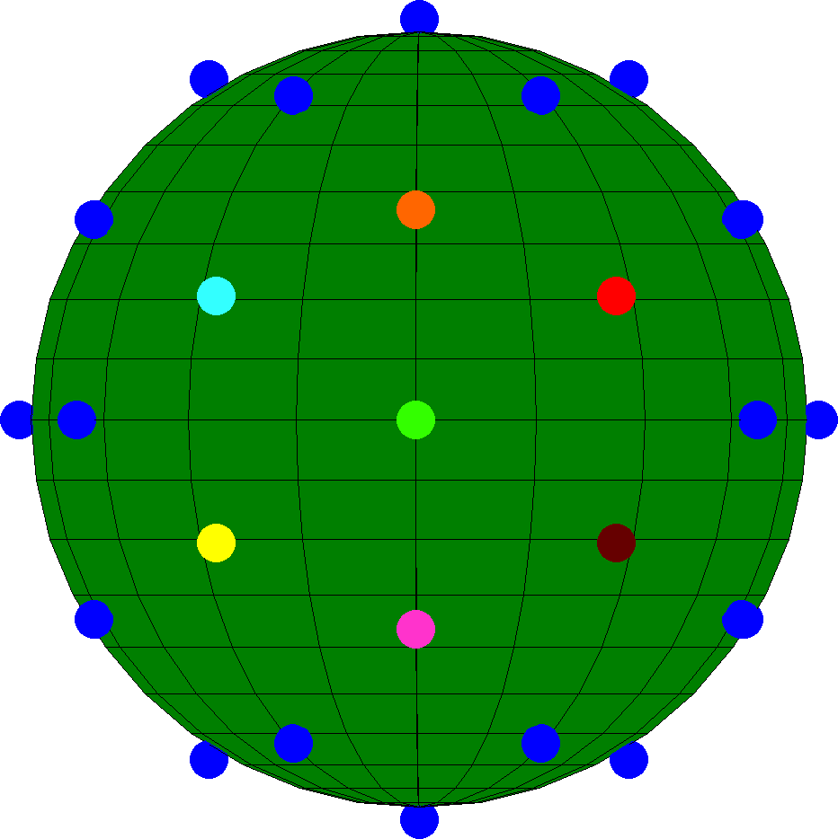
We now define two important terms used throughout the present work. Firstly, a patch is defined as a 3D region of neighboring spatial voxels, i.e. a small local region of a single 3D DWI. Secondly, a block is defined as a collection of patches taken at the same spatial position, but in different DWIs, i.e. a block is a 4D stack of patches which are similar in the angular domain. The reader is referred to Fig. 1 for a visual representation of the process.

(a) A block is made of the b0 and some angular neighbors

(b) Angular neighbors position on the sphere.

Figure 1: a) A 3D block is made by stacking along the 4th dimension the b0, a DWI and its angular neighbors, which share similar structure, but under a slightly different noise realization. b) Disposition of equidistant angular neighbors on the sphere.

The Block Matching Algorithm

Reusing the key ideas from the non local means, the block matching algorithm (Dabov et al., 2007) further exploits image self-similarity. Similar 2D patches found inside a local neighborhood are stacked into a 3D transform domain and jointly filtered via wavelet hard-thresholding and Wiener filtering. Combining these filtered estimates using a weighted average based on their sparsity leads to superior denoising performance than the non local means filter. The idea has been extended in 3D for MRI image denoising in (Maggioni et al., 2013) and an adaptive patch size version for cardiac diffusion MRI image denoising was successfully employed by (Bao et al., 2013).

The Dictionary Learning Algorithm

Dictionary learning has been used in the machine learning community to find data driven sparse representations (Elad and Aharon, 2006; Mairal et al., 2009). Typically, a set of atoms (called the dictionary) is learned over the data, providing a way to represent it with a basis tailored to the signal at hand (Olshausen and Field, 1996). This is analogous to using an off-the-shelf basis like the discrete cosine transform or wavelets, but in a data-driven manner which gives better results than using a fixed, general purpose basis. The main difference is that this is not necessarily a basis in the sense it can also be overcomplete, i.e. it can have more atoms than coefficients. Given a set of input data $\mathbf{X}=[x_{1},\dots,x_{n}]\in\mathbb{R}^{m\times n}$ organized as column vectors, the process is expressed as

$$\min_{\mathbf{D},\boldsymbol{\alpha}}\frac{1}{n}\sum_{i=1}^{n}\left(\frac{1}{2}\left\lVert x_{i}-\mathbf{D}\alpha_{i}\right\rVert_{2}^{2}+\lambda\left\lVert\alpha_{i}\right\rVert_{1}\right)\enspace\text{s.t.}\enspace\left\lVert\mathbf{D}\right\rVert_{2}^{2}=1\enspace,$$ (1)

where $\mathbf{D}\in\mathbb{R}^{m\times p}$ is the learned dictionary, $\lambda$ is a trade-off parameter between the data fidelity term and the penalization on the coefficients $\boldsymbol{\alpha}=[\alpha_{1},\dots,\alpha_{n}]\in\mathbb{R}^{p\times n}$. A higher value of $\lambda$ promotes sparsity at the expense of the similarity with the original data. The columns of $\mathbf{D}$ are also constrained to be of unit $\ell_{2}$ norm in order to avoid degenerated solutions (Mairal et al., 2009; Elad and Aharon, 2006; Gramfort et al., 2014). The key is to devise a sparse representation to reconstruct structural information and discard noise, since the latter does not typically allow a sparse representation in any basis. Using a penalization on the $\ell_{1}$ norm of the coefficients promotes sparsity, hence providing denoising through the regularized reconstruction. This idea has led to inpainting and denoising applications from the machine learning community (Mairal et al., 2009; Elad and Aharon, 2006) or even to accelerated acquisition process in the diffusion MRI community for diffusion spectrum imaging (DSI) (Gramfort et al., 2014).

Adjusting for various noise types

Although the original formulations of Eq. (1) and Eq. (4) assume stationary, white additive Gaussian noise, this is usually not true in diffusion MRI data, especially at high b-values and low SNR. The noise is usually modeled as following a Rician distribution or a nc-$\chi$ distribution when used with parallel imaging depending on the reconstruction algorithm and the number of coils N used during the acquisition (Dietrich et al., 2008; Aja-Fernández et al., 2014). This introduces a bias which depends on the intensity of the signal that must be taken into account to recover the expected value of the original signal as shown in Fig. 2. Note, though, that other common preprocessing corrections, such as motion correction or eddy current correction, require interpolation and could thus change the theoretical noise distribution (Veraart et al., 2013).

Figure 2: Top : a) A noisy acquisition with slowly varying nc-$\chi$ noise and b) the resulting stabilized, Gaussian distributed noisy DWI. c) A noisy acquisition with fast varying Rician noise where the background was masked by the scanner with d) its stabilized counterpart. Bottom : Histogram of the nc-$\chi$ noise distribution in the selected background region of a) before stabilization and b) after stabilization. Note the non-Gaussianity of the noise in a) versus b).

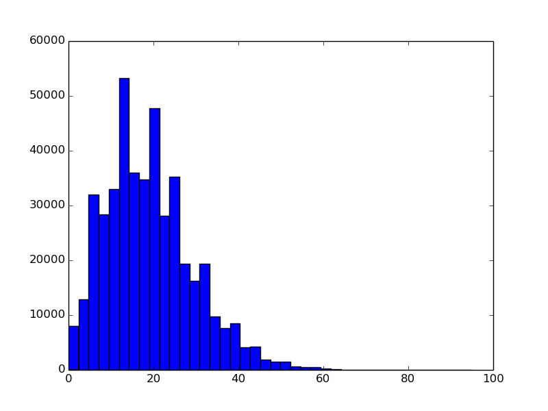
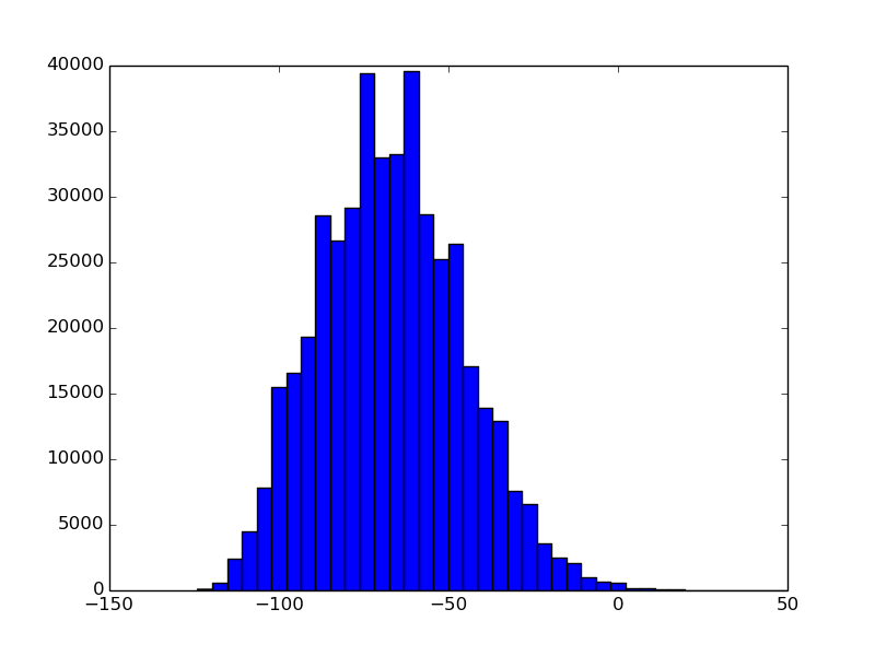
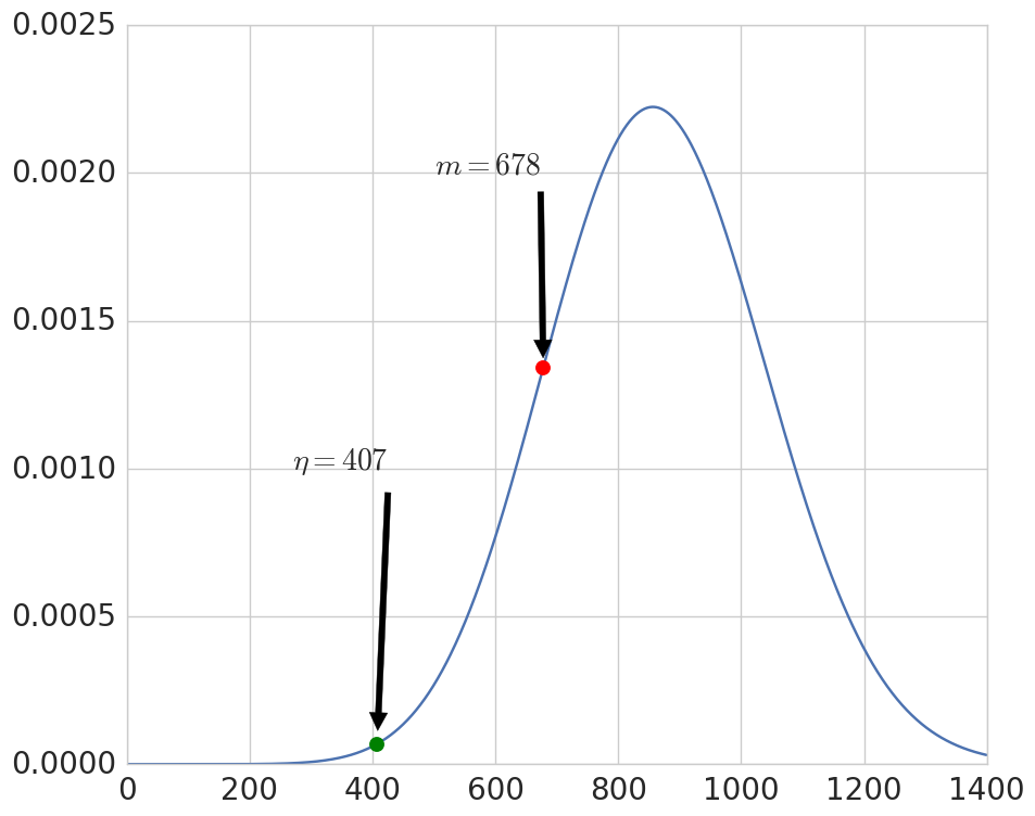
The key idea lies in the fact that the nc-$\chi$ distribution is actually made from a sum of Gaussians, from which the Rician distribution is a special case with N = 1. By making the hypothesis that each of the 2N Gaussian distributions share the same standard deviation $\sigma_{G}$ (Koay et al., 2009a), one can map a value $m$ from a nc-$\chi$ distribution to an equivalent value $\hat{m}$ from a Gaussian distribution. We first compute estimates for $\sigma_{G}$ and $\eta$ (which is an estimate of the signal value in a Gaussian setting). If $\eta$ is below the noise floor due to a low local SNR, that is when $\eta<\sigma_{G}\sqrt{\pi/2}$, we set $\eta=0$ instead of being negative as suggested by (Bai et al., 2014). The next step uses the cumulative distribution function (cdf) of a nc-$\chi$ distribution and the inverse cumulative distribution function (icdf) of a Gaussian distribution to find the equivalent value $\hat{m}$ between the two distributions. This effectively maps a noisy nc-$\chi$ distributed signal $m$ to an equivalent noisy Gaussian distributed signal $\hat{m}$. See Fig. 3 for a synthetic example with a visual depiction of the process for mapping nc-$\chi$ signals to Gaussian distributed signals and (Koay et al., 2009a) for the original in-depth details.

(a) pdf of nc-$\chi$ distribution.

(b) cdf of nc-$\chi$ distribution.

(c) icdf of Gaussian distribution.

Figure 3: A synthetic example of the stabilization algorithm. a) Given a noisy value $m=678$ observed in a nc-$\chi$ distribution with $N=4$ and $\sigma_{G}=200$, the underlying value is estimated as $\eta=407$. b) The associated probability in the nc-$\chi$ cdf with $\eta$ is $\alpha=0.513$, c) thus giving from the inverse cdf of a Gaussian distribution with mean $\mu=407$ and standard deviation $\sigma_{G}=200$ a new noisy value $\hat{m}=413$.

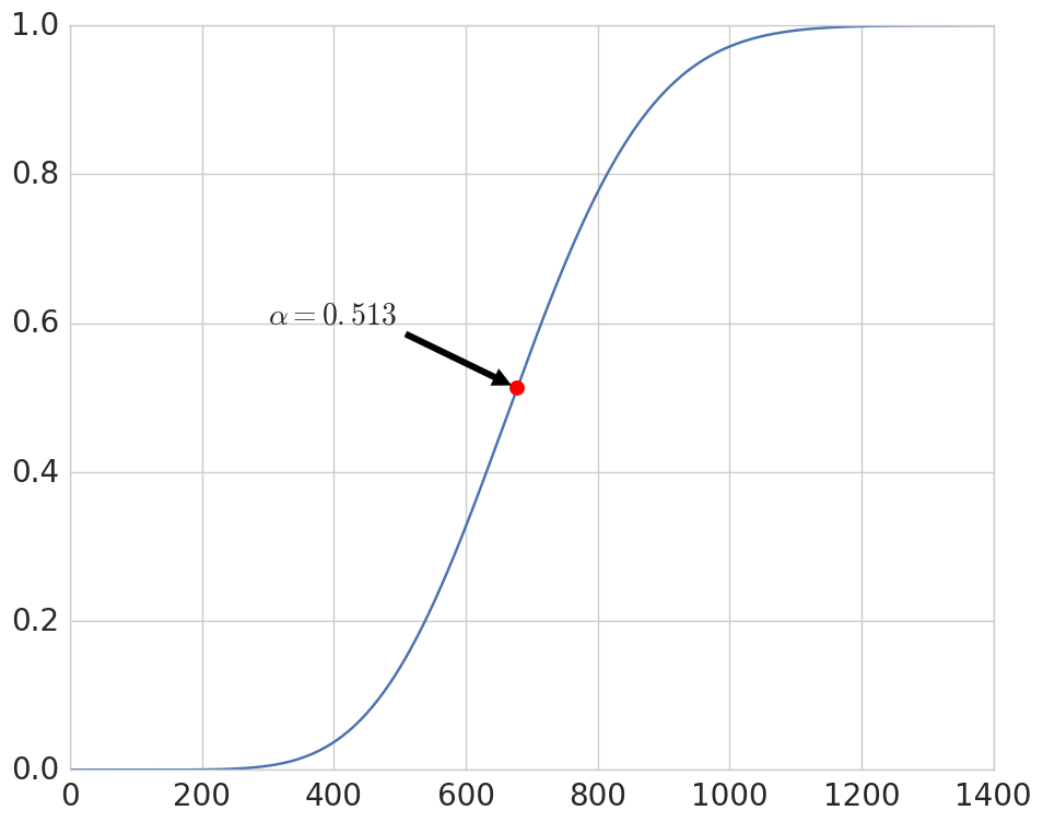
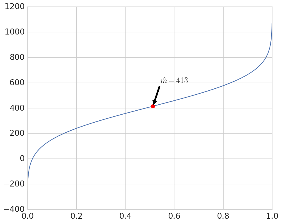
Using a variance stabilization means considering the noise as additive white Gaussian noise, which allows any already designed technique for Gaussian noise to be used without any modification. The author of (Foi, 2011) has shown that techniques with a Rician noise adaptation performed equally well as their Gaussian noise version through the use of a noise stabilization approach. The same idea has been directly applied with block matching  (Dabov et al., 2007) for structural MRI in (Maggioni et al., 2013). The classical solution to remove the noise bias is to include the noise model into the denoising algorithm itself, as for example done in  (Aja-Fernandez et al., 2008; Becker et al., 2014; Lam et al., 2014; Manjón et al., 2010). The drawback with this solution is that each method has to be rethought to account for any other noise type not considered in its original formulation.

3 Method

Adjusting for various noise types

In this paper, we will deal with both the Rician and nc-$\chi$ noise model on a voxelwise basis through the noise stabilization technique of (Koay et al., 2009a). This indeed makes our algorithm easily adaptable for any noise type by simply changing the pre-applied transformation as needed. We will use the Probabilistic Identification and Estimation of Noise (PIESNO) (Koay et al., 2009b) to estimate the stationary noise standard deviation. PIESNO works on a slice by slice basis, assuming the background noise as stationary along the selected slice, and is designed to find the underlying standard deviation of the Gaussian noise given its Rician or nc-$\chi$ nature. Voxels that are considered as pure background noise are found automatically by the method, using the fact that the squared mean of those voxels follows a Gamma distribution. Once automatically identified, the standard deviation $\sigma_{G}$ of those voxels can be computed and a new estimation of the Gamma distribution is made with the updated $\sigma_{G}$ until convergence. In the case of spatially varying noise, we will use a method similar to (Manjón et al., 2010), where the noise is estimated locally as

$$\sigma^{2}_{i}=\min||u_{i}-u_{j}||_{2}^{2},\forall i\neq j,$$ (2)

with $u_{i}$ a noisy patch computed by subtracting a patch to a low-pass filtered version of itself and applying the local Rician correction factor of (Koay and Basser, 2006). If the background was masked automatically by the scanner or is unreliable due to the scanner preprocessing for statistical estimation, we use a similar idea by computing the local standard deviation of the noise field as

$$\sigma_{i}=\text{std}(u_{i}-\text{low\rule{4.30554pt}{0.4pt}pass}(u_{i}))$$ (3)

If a noise map was acquired during the scanning session, it can be sampled directly to estimate the parameters of the noise distribution. In the event that such a map is unavailable, a synthetic one can be constructed by subtracting the image from its low-pass filtered counterpart (see Eq. 3). Since the noise is assumed as independent and identically distributed across DWIs, we apply a median filter on the 4D dataset to get a 3D noise field. Finally, a Gaussian filter with a full-width at half maximum of 10 mm is applied to regularize the noise field, which is then corrected for the more general nc-$\chi$ bias with the correction factor of (Koay and Basser, 2006). A similar approach based on extracting the noise field with a principal component analysis was used by (Manjón et al., 2013).

Locally Adapting the Dictionary Learning

In order to locally adapt the method to spatially varying noise, we add some more constraints to the classical formulation of Eq. (1). Firstly, since the measured signal in diffusion MRI is always positive, we use this assumption to constrain the positivity of the global dictionary $\mathbf{D}$ and the coefficients $\boldsymbol{\alpha}$, i.e. $\mathbf{D}\geq 0,\boldsymbol{\alpha}\geq 0$ as done in (Gramfort et al., 2014). We fixed the regularization parameter $\lambda$ for Eq. (1) in the same fashion as (Mairal et al., 2009), that is $\lambda=1.2/\sqrt{m}$, with $m=ps^{3}\times an$, $ps$ is the patch size and $an$ the number of angular neighbors. Secondly, once $\mathbf{D}$ is known, we use Eq. (4) (see the next paragraph) iteratively until convergence with the constraint $\boldsymbol{\alpha}\geq 0$ and $\lambda_{i}=\sigma_{i}^{2}(m+3\sqrt{2m})$, where $\sigma^{2}_{i}$ is the local noise variance found either with PIESNO or Eq. (3). In accordance with (Candès et al., 2008), $\lambda_{i}$ is an upper bound on the $\ell_{2}$ norm of the noise. We set the convergence as reached for $\alpha_{i}$ at iteration $j$ when $\max|\alpha_{i,j}-\alpha_{i,j-1}|<10^{-5}$ or until a maximum of 40 iterations is realized.

Adaptive and Iterative $\ell_{1}$ Minimization

While Eq. (1) will both construct the dictionary $\mathbf{D}$ and find the coefficients $\boldsymbol{\alpha}$, there are specialized iterative algorithms for solving $\ell_{1}$ problems in order to yield sparser solutions (Daubechies et al., 2010; Candès et al., 2008). An equivalent constrained formulation for solving each column $i$ of $\boldsymbol{\alpha}$ is

$$\min_{\alpha_{i}}\left\lVert w_{j}\alpha_{i}\right\rVert_{1}\enspace\text{s.t.}\enspace\frac{1}{2}\left\lVert x_{i}-\mathbf{D}\alpha_{i}\right\rVert_{2}^{2}\leq\lambda_{i},$$ (4)

where $w_{j}$ is a weighting vector penalizing the coefficients of $\alpha_{i}$ at iteration $j$. Eq. (4) can thus be iterated to further identify non zero coefficients in $\alpha_{i}$ by setting $w_{j+1}=\frac{1}{\lvert\alpha_{i}\rvert+\epsilon}$ for the next iteration. The algorithm is then started with $w_{0}=1$ and $\epsilon=\max\lvert\mathbf{D}^{T}\xi\rvert$. As suggested by (Candès et al., 2008), $\xi\sim\mathcal{N}(0,\sigma^{2})$ is set as a random Gaussian vector, which gives a baseline where significant signal components might be recovered. While similar in spirit to Eq. (1), Eq. (4) provides a way to find the sparser representation for $\alpha_{i}$ while bounding the $\ell_{2}$ reconstruction error.

To the best of our knowledge, our paper is also the first to use the noise variance as an explicit bound on the $\ell_{2}$ reconstruction error. This yields a sparse representation while controlling at the same time the fidelity with respect to the original data, while the classical way is to use the variance as a regularized penalization factor.

3.1 The proposed algorithm

Our new NLSAM algorithm combines ideas from block matching and sparse coding. We will use the same kind of framework, but by replacing the thresholding part in the block matching with a step of dictionary denoising instead, allowing the penalization on the sparsity of the signal to regularize the noisy blocks. We also take explicit advantage of the fact that diffusion MRI data is composed of multiples volumes of the same structure, albeit with different noise realizations and contrasts across DWIs. This allows sparser estimates to be found, further enhancing the separation of the data from the noise (Olshausen and Field, 1996). Our method is thus composed of three steps :

1. Correct the noise bias if needed.

2. Find angular neighbors on the sphere for each DWI.

3. Apply iterative local dictionary denoising on each subset of neighbors.

Step 1. In case the noise is not Gaussian distributed, we first correct for the noise bias by finding the Gaussian noise standard deviation with PIESNO (Koay et al., 2009b). If the background is masked, we instead use Eq. (3). We then transform the DWIs into Gaussian distributed, noisy signals using the correction scheme of (Koay et al., 2009a).

Step 2. We find the angular neighbors for each of the DWIs. In this step, the local angular information is encoded in a 4D block of similar angular data, as seen in Fig. 1. The gradients are symmetrized to account for opposite polarity DWIs, which share similar structure to their symmetrized counterpart. The search is also made along all the shell at the same time, since structural information (such as sharp edges) is encoded along the axial part of the data. This encodes the similar angular structure of the data along the 4th dimension in a single vector.

Step 3. The dictionary D is constructed with Eq. (1) and the blocks are then denoised with Eq. (4). This step can be thought of finding a linear combination with the smallest number of atoms to represent a block. In order to adapt to spatially varying noise, each block is penalized differently based on the local variance of the noise. This enables the regularization to adapt to the amount of noise in the block, which is usually stronger as the acquired signal is farther from the receiver coils. Since each overlapping block is extracted, each voxel is represented many times and they are recombined using a weighted average based on their sparsity as in (Manjón et al., 2013; Maggioni et al., 2013). For each voxel $i$ with intensity $v_{i}$ contained in multiple overlapping blocks $V_{j}$ in neighborhood $V$, we set the final value of $v_{i}$ as

$$v_{i}=\frac{\sum\limits_{j\in V}v_{j}(1+||V_{j}||_{0})}{\sum\limits_{j\in V}1+||V_{j}||_{0}},$$ (5)

where $V$ is the same spatial position for voxel $i$ across multiple blocks $V_{j}$. This assumes that more coefficients in block $V_{i}$ also means more noise in the reconstruction. The $\ell_{0}$ norm thus penalizes reconstructions with more coefficients and assigns a lower weight in that case for the overlapping weighted average.

This third step is then repeated for all the DWIs. Since each DWI will be processed more than once with a different set of neighbors each time (see Fig. 1 for the block formation process), we obtain multiple denoised volumes of exactly the same data, but denoised in a different angular context. Once all the DWIs have been processed, we average the multiple denoised versions obtained previously in order to further reduce any residual noise. See A for an outline of the NLSAM algorithm as pseudocode. The result will be a denoised version of the input, through both dictionary learning and spatial and angular block matching.

3.2 Datasets and acquisition parameters

Synthetic phantom datasets

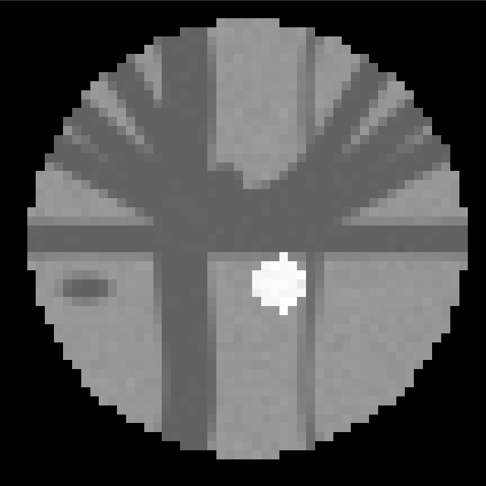
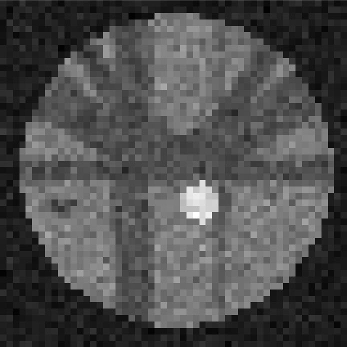
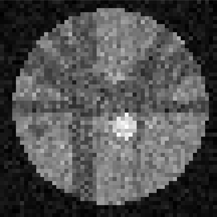
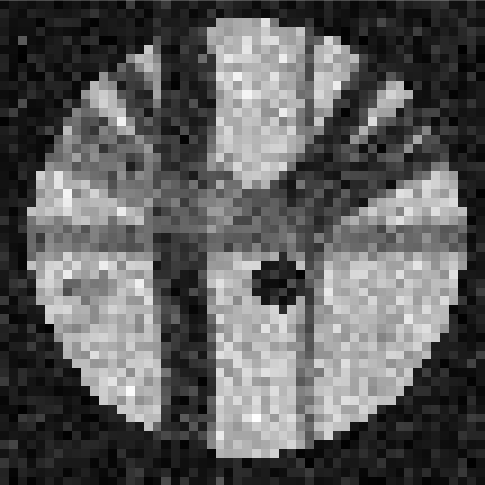
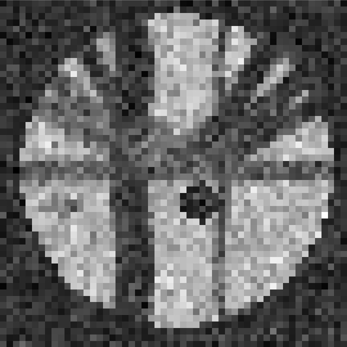
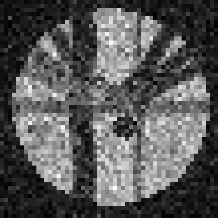
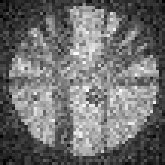
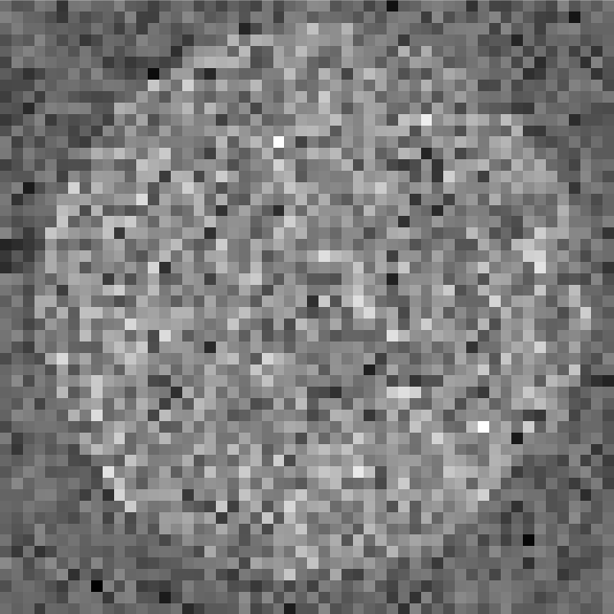
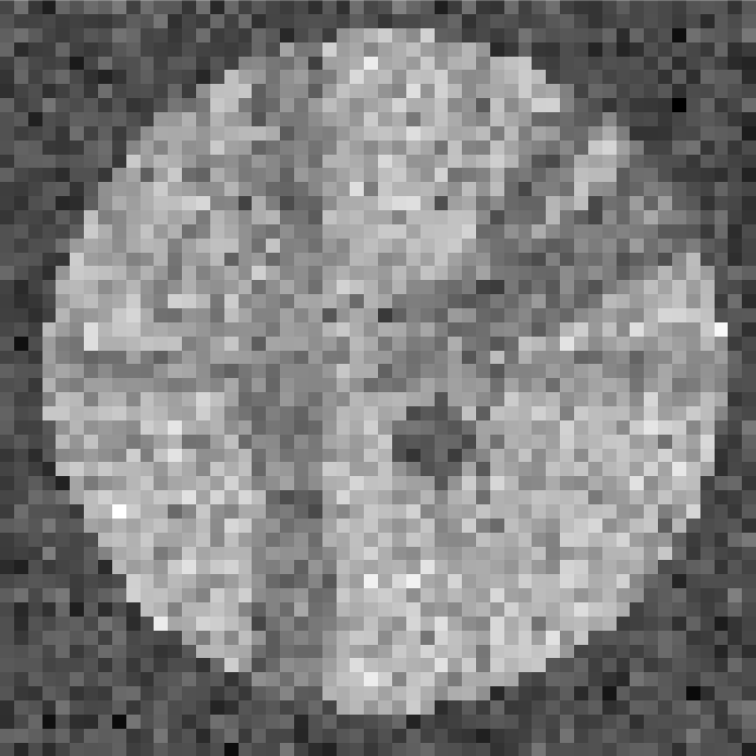
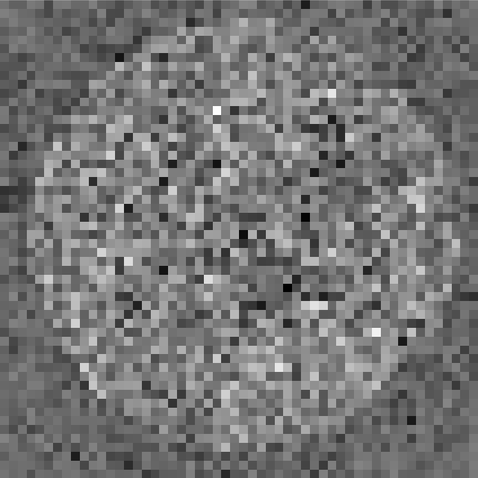
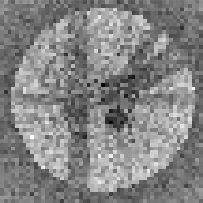
The synthetic data simulations are based on the ISBI 2013 HARDI challenge phantom and were made with phantomas. We used the given 64 gradients set from the challenge at b-values of 1000 and 3000 s/mm². For simplicity, we will now refer to these datasets as the b1000 and the b3000 datasets. The datasets were generated with Rician and nc-$\chi$ noise profile, both stationary and spatially varying, at two different signal-to-noise ratios (SNR) for each case. In total, we thus have 8 different noise profiles for each b-value. The stationary noise was generated with SNR 10 and 20 and the spatially varying noise was generated with SNR varying linearly from 5 to 15 and from 7 to 20. The noise distributions were generated for each SNR by setting $N=1$ for the Rician noise and $N=12$ for the nc-$\chi$ noise. The noisy data was generated according to

$$\hat{I}=\sqrt{\sum_{i=0,j=0}^{N}\left(\frac{I}{\sqrt{N}}+\beta\epsilon_{i}\right)^{2}+\beta\epsilon_{j}^{2}},\enspace\mbox{where }\epsilon_{i},\epsilon_{j}\sim\mathcal{N}(0,\sigma^{2}),$$ (6)

where $\hat{I}$ is the resulting noisy volume, $\mathcal{N}(0,\sigma^{2})$ is a Gaussian distribution of mean 0 and variance $\sigma^{2}$ with $\sigma$ = mean (b0) / SNR and mean(b0) is the mean signal value of the b $=0$ s/mm² image. $\beta$ is a mask to create the noise distribution set to 1 in the constant noise case and as a sphere for the spatially varying noise case. For the spatially varying noise experiments, $\beta$ has a value of 1 on the borders up to a value of 3 at the middle of the mask, thus generating a stronger noise profile near the middle of the phantom than for the stationary (constant) noise case. As shown on Fig. 4, this results in a variable SNR ranging from approximately SNR 5 and SNR 7 in the middle of the phantom up to SNR 15 and SNR 20 for the spatially varying noise case. This noise mimics a homogeneous noise reconstruction as implemented by some scanners while still having a spatially varying noise map.

b0 image

DW image

Added noise g

(a) Noiseless

(b) SNR10 stat Rician

(c) SNR10 stat nc-$\chi$

(d) SNR15 var Rician

(e) SNR15 var nc-$\chi$

Figure 4: Synthetic b1000 datasets with various noise profiles used in the experiments. The top row shows the b0 image, the middle row shows the same DWI across noise types and the bottom row shows the various noise distribution which generated the middle row. From left to right : the noiseless data, SNR 10 with stationary Rician noise, SNR 10 with stationary nc-$\chi$ noise, SNR 15 with spatially variable Rician noise, SNR 15 with spatially varying nc-$\chi$ noise.

Real datasets

In order to compare our NLSAM method on a real dataset, we acquired a full brain in-vivo dataset consisting of 40 DWIs at $\mbox{b}=1000\mbox{ s/mm}^{2}$ and one $\mbox{b}=0\mbox{ s/mm}^{2}$. The acquisition spatial resolution was $1.2\times 1.2\times 1.2\mbox{ mm}^{3}$, TR/TE = 18.9 s / 104 ms, gradient strength of 45 mT/m on a 3T Philips Ingenia scanner with a 32 channels head coil for a total acquisition time of 13 minutes. An in-plane parallel imaging factor of R = 2 was used with the SENSE reconstruction algorithm, thus giving a fast spatially varying Rician noise distribution (hence, the denoising algorithms will be set with $N=1$) even if multiple coils are used by the reconstruction algorithm for producing the final image (see Fig. 2). No correction was applied to the dataset, as we wanted to show the effectiveness of denoising without any other preprocessing step such as eddy current or motion correction, which could introduce blurring caused by interpolation. To obtain a comparable clinical-like baseline dataset and show the advantage of acquiring directly high resolution DWIs, we also obtained a 64 DWIs dataset at $\mbox{b}=1000\mbox{ s/mm}^{2}$ and one $\mbox{b}=0\mbox{ s/mm}^{2}$ of the same subject. The spatial resolution was $1.8\times 1.8\times 1.8\mbox{ mm}^{3}$, TR/TE = 11.1 s / 63 ms, for a total acquisition time of 12 mins. The acquisition was made on the same scanner, but during another scanning session. No further processing nor denoising was done on this dataset for the reasons mentioned above. This can be thought of having a higher angular resolution at the cost of a lower spatial resolution for a comparable acquisition time.

3.3 Other denoising algorithms for comparison

We now present the various features and cases covered by the denoising algorithms studied in this paper. The Adaptive Optimized Nonlocal Means (AONLM) method (Manjón et al., 2010) is designed for Rician noise removal in a 3D fashion and works separately on each DWIs volume. It also includes a Rician bias removal step and is able to spatially adapt to a varying noise profile automatically. We used the recommended default parameter of a 3D patch size of 3 x 3 x 3 voxels with the Rician bias correction in all cases. The Local Principal Component Analysis (LPCA) method (Manjón et al., 2013) is also made to take into account the Rician noise bias and is spatially adaptive, but also uses the information from all the DWIs in the denoising process. We used the automatic threshold set by the method with the Rician noise correction for all experiments. Both AONLM and LPCA can be downloaded from the author’s website. The multi-shell Position-Orientation Adaptive Smoothing (msPOAS) algorithm (Becker et al., 2014) was designed for both Rician and nc-$\chi$ noise, while also taking into account the angular structure of the data for adaptive smoothing. We discussed with the authors of msPOAS for their recommendations and using their suggestion, we set $k^{\star}=12$ and $\lambda=18$. We also supplied the correct value for $N$ and used the implemented automatic detection of the noise standard deviation from msPOAS. For the NLSAM algorithm, we used a patchsize of 3 x 3 x 3 voxels with 4 angular neighbors, which corresponds to the number of angular neighbors at the same distance on the sphere for each selected DWI. The value of $N$ was given to the algorithm and the number of atoms was set to two times the number of voxels in a block for the dictionary learning part, which was repeated for 150 iterations. The other parameters were set as described in Section 3. As shown in Table 1, our method is designed to work on both stationary and spatially variable Rician and nc-$\chi$ noise. The NLSAM algorithm is implemented in python and is also freely available.

Finally, we quantitatively assess the performance of each method by comparing them against the noiseless synthetic data using

1. The peak signal-to-noise ratio (PSNR) in dB and the structural similarity index (SSIM) on the raw data intensities (Wang et al., 2004).

2. The dispersion of the FA error, computed from a weighted least-square diffusion tensor model.

3. The mean angular error (AE) in degrees and the discrete number of compartments (DNC) error for a region of crossings (Daducci et al., 2014; Paquette et al., 2014).

4. The Tractometer (Côté et al., 2013) ranking platform on deterministic tractography algorithms for the synthetic datasets. This platform computes global connectivity metrics, giving an insight on the global coherence of the denoised datasets in a tractography setting.

5. Tracking some known bundles on the high resolution in-vivo dataset and qualitatively comparing them to their lower spatial resolution counterpart.

3.4 Local models reconstruction and fiber tractography

The weighted least-square diffusion tensors were reconstructed using the default parameters of Dipy (Garyfallidis et al., 2014) to compute the FA values. We used the Constrained Spherical Deconvolution (CSD) (Tournier et al., 2007) with a spherical harmonics of order 8 to reconstruct the fODFs and extract the peaks subsequently used for the deterministic tracking. To compute the fiber response function (frf), we used all the voxels in the white matter that had an FA superior to 0.7. If less than 300 voxels meeting this criterion were found, the FA threshold was lowered by 0.05 until the criterion was met. See Sections 4.2 and 5.3 for more information about the bias introduced in the FA. For the synthetic datasets, the tracking was done inside the white matter mask and the seeding was done from the bundles extremities to mimic seeding from the white-gray matter interface (Girard et al., 2014). We used 100 seeds per voxels to allow sufficient bundle coverage, a stepsize of 0.2 mm and a maximum angle deviation of 60 degrees. The other parameters used were the defaults supplied by the tractometer pipeline (Côté et al., 2013). The in-vivo datasets deterministic tracking was made with the technique of (Girard et al., 2014) by seeding from the white matter and gray matter interface with the particle filtering and generating approximately 1 million of streamlines. White matter masks were created by segmenting a T1 image with FSL FAST from the same subject and then registered with ANTs to each in-vivo dataset. The bundles were finally automatically segmented using the White Matter Query Language (WMQL) (Wassermann et al., 2013) Tract Querier tool with regions obtained from a T1 white matter and gray matter parcellation. This atlas-based automatic dissection method extracts fiber bundles automatically using anatomical definitions in a reproducible manner for all methods, as opposed to the traditional way of manually defining including and excluding ROIs to define bundles. Visualization of fODFs, peaks and tractography was made using the fibernavigator (Chamberland et al., 2014).

4 Results

4.1 Preserving the raw DWI data

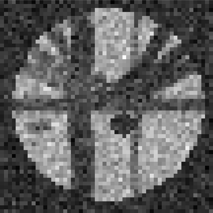
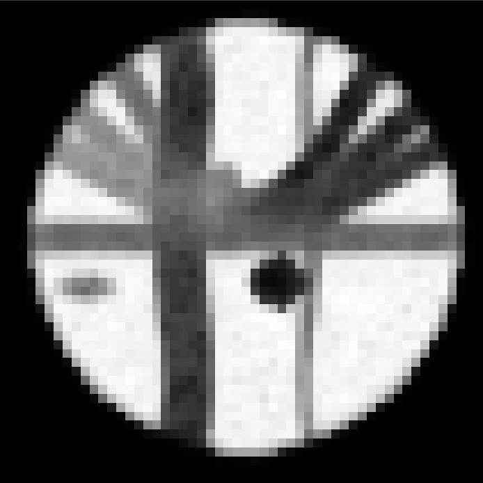
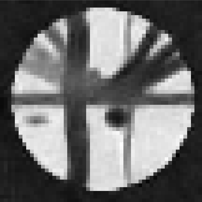
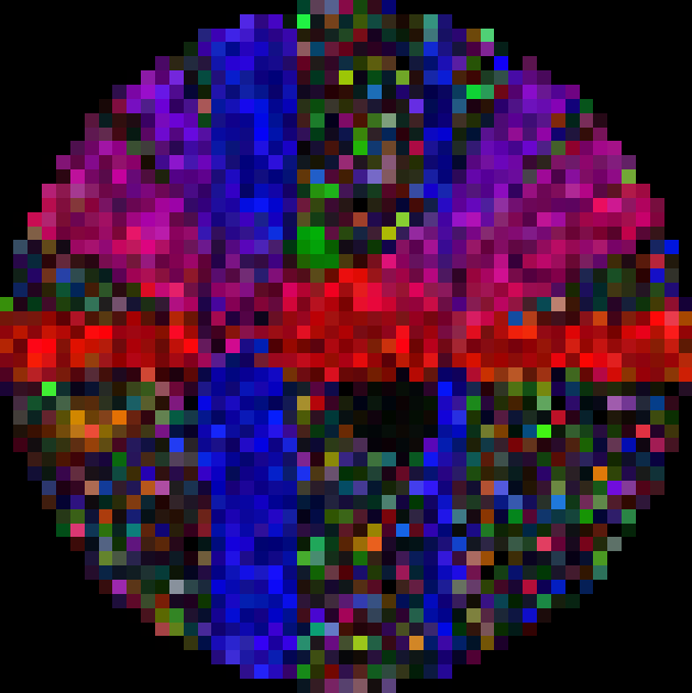
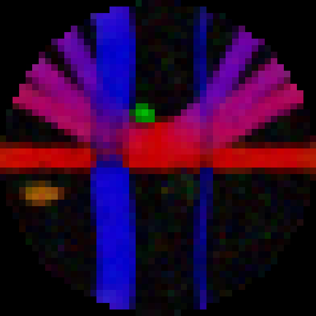
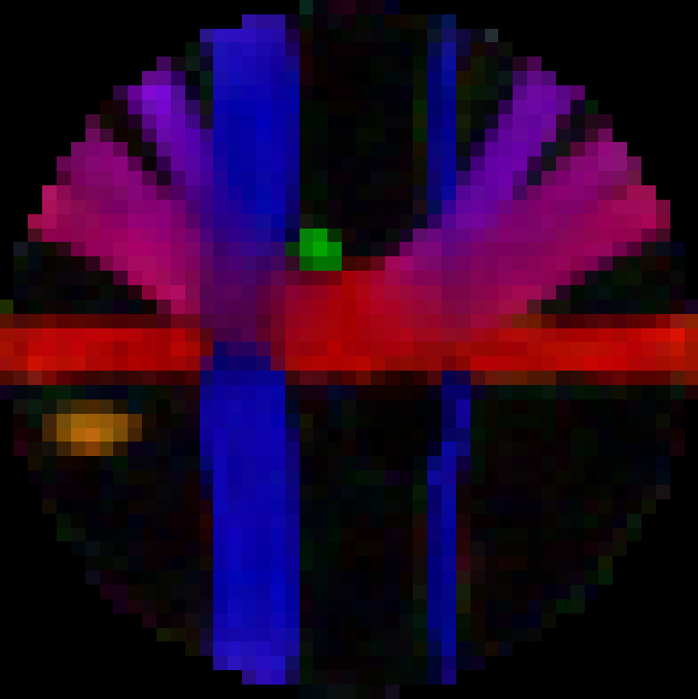
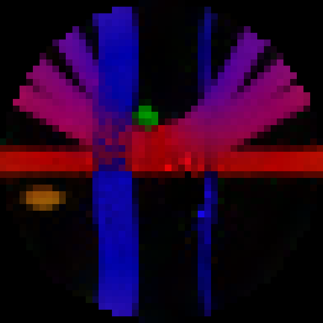
Fig. 5 (displayed in landscape to see all the compared methods on the same figure) shows the b1000 noiseless data, the noisy input data at SNR 10 for nc-$\chi$ stationary noise and the results of the denoising on the synthetic phantom for all compared methods. This is the noise case theoretically covered by msPOAS and our NLSAM algorithm. We also show two zoomed regions of crossings with the reconstructed peaks extracted from fODFs. All perceptual and FA metrics were computed on the slice shown while angular metrics were computed in the zoomed region depicted by the yellow box. Note how the small blue bundle and its crossings are preserved on the NLSAM denoised dataset, while other denoising methods tend to introduce blurring.

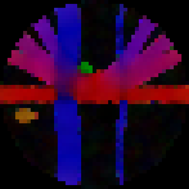
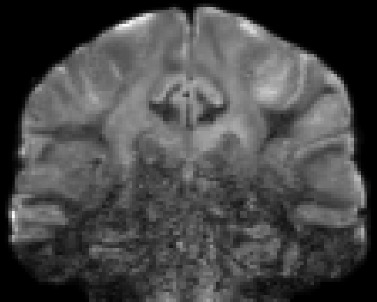
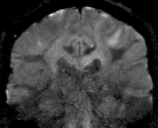
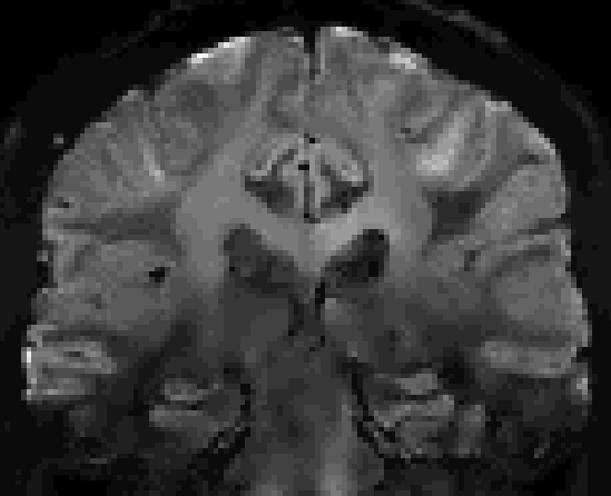
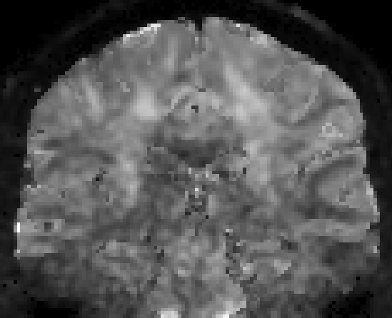
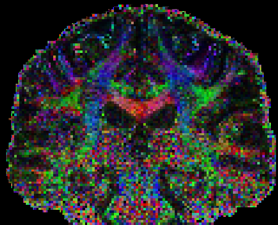
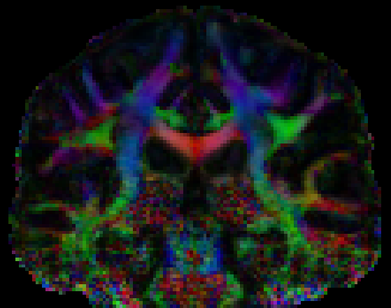
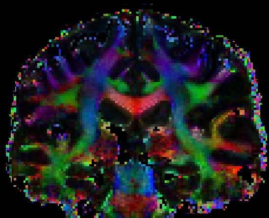
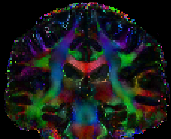
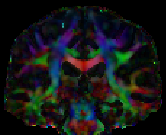
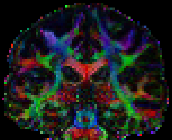
Fig. 6 (also in landscape for enhanced viewing) shows the noisy high resolution in-vivo dataset, the denoised version obtained for each algorithm and the low spatial resolution acquisition of the same subject without any denoising. Since our scanner uses a 32 channels head-coil but implements the SENSE reconstruction algorithm, the resulting spatially varying Rician noise distribution is the case covered by AONLM, LPCA and our NLSAM algorithm. We show a coronal slice for the gradient direction closest to (0, 1, 0), the colored FA map and a zoom on two regions of crossings. The yellow region shows the junction of the corticospinal tract (CST) and superior longitudinal fasciculus (SLF) while the white region shows the junction of the corpus callosum (CC) and the CST. While the high resolution dataset is noisier than its lower resolution counterpart, the highlighted crossings regions are well recovered by the denoising algorithms and thus offer an improvement in anatomical details over the lower spatial resolution dataset. We also see in the yellow box that the NLSAM denoised dataset recovers crossings extending from the CC which are almost absent in the compared datasets.

(a) Noiseless

(b) Noisy

(c) NLSAM

(d) AONLM

(e) LPCA

(f) msPOAS

Figure 5: Phantomas b1000 synthetic dataset at SNR 10 for stationary nc-$\chi$ noise on the y = 24 slice. From top to bottom : Raw diffusion MRI, colored FA map, zoom on extracted peaks from fODF of order 8. Note how NLSAM restores the structure without blurring on the colored FA map and is the only method to restore the peaks from the noisy dataset in the zoomed white box region.

0

(a) Noisy 1.2 mm

(b) NLSAM

(c) AONLM

(d) LPCA

(e) msPOAS

(f) Noisy 1.8 mm

Figure 6: From top to bottom, the raw high resolution in-vivo data corrupted with spatially varying Rician distributed intensities, the colored FA map and a zoom on two regions of crossings. All denoised methods were applied on the high spatial resolution 1.2 mm dataset. We also show an acquisition of the same subject at 1.8 mm for visual comparison. Our NLSAM algorithm is able to recover more crossings from the 3 way junction of the SLF, the CST and the CC as shown in the yellow and white boxes. While the 1.8 mm dataset is less noisy, its lower spatial resolution also means that each voxel contains more heterogeneous tissues and mixed diffusion orientations. The 1.2 mm denoised dataset shows more crossings without the averaging effect of the larger voxel size. For a comparable acquisition time, the denoised high resolution dataset has more information than its lower resolution counterpart without processing.

0

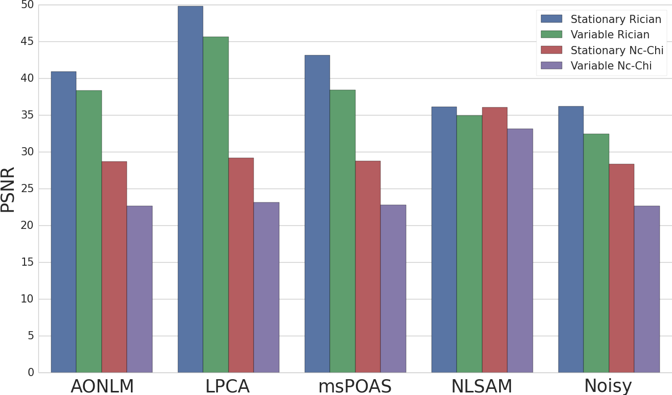
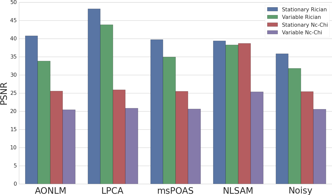
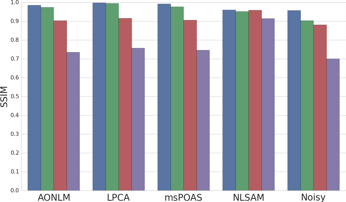
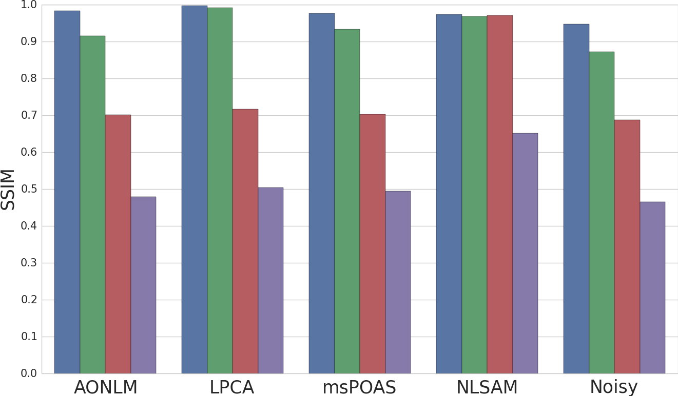
Fig. 7 shows the PSNR and SSIM for the SNR 10 (stationary noise) and SNR 15 (spatially varying noise) synthetic datasets. The LPCA algorithm performs best in term of PSNR on the Rician noise case, but attains a lower score for nc-$\chi$ noisy datasets. The same trend is seen for AONLM and msPOAS algorithms, where the SNR 15 nc-$\chi$ case is the hardest test case. In contrast, our NLSAM technique is above 30 dB for the PSNR and 0.9 for the SSIM in most cases, with a relatively stable performance amongst the majority of tested cases. We also note that even though msPOAS is made to adjust itself to nc-$\chi$ noise, the fact that the algorithm does not account for the intensity bias makes the perceptual metrics drop for the nc-$\chi$ noise cases.

(a) PSNR b1000

(b) PSNR b3000

(c) SSIM b1000

(d) SSIM b3000

Figure 7: PSNR and SSIM metrics for the SNR 10 stationary and SNR 15 spatially variable noise cases datasets. All methods can correct the stationary and spatially varying Rician noise case to some extent while only our NLSAM algorithm has the best performance for the nc-$\chi$ noise case, especially for the spatially varying noise case.

4.2 Bias introduced in the FA

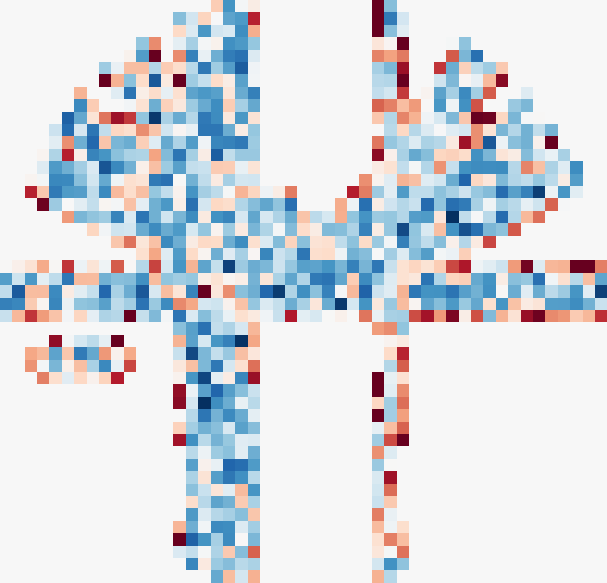
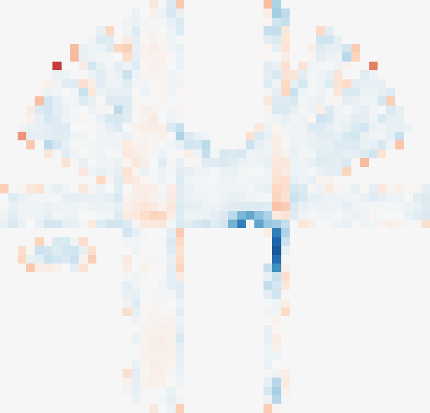
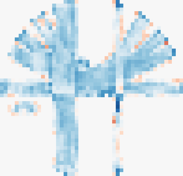
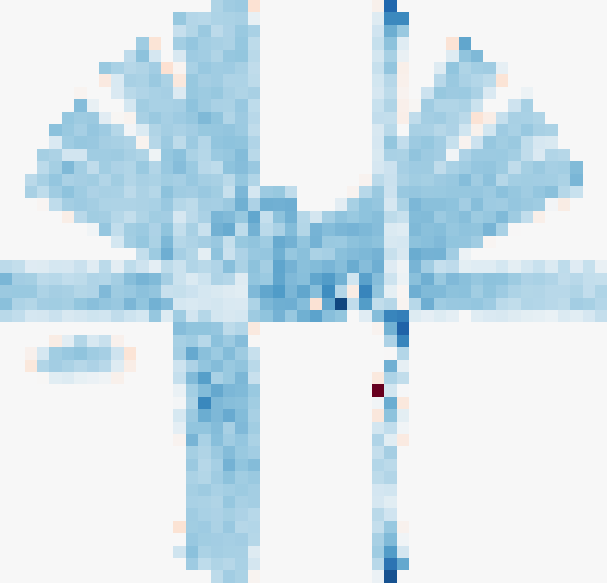
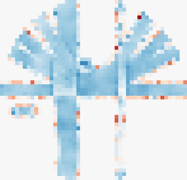
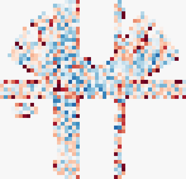
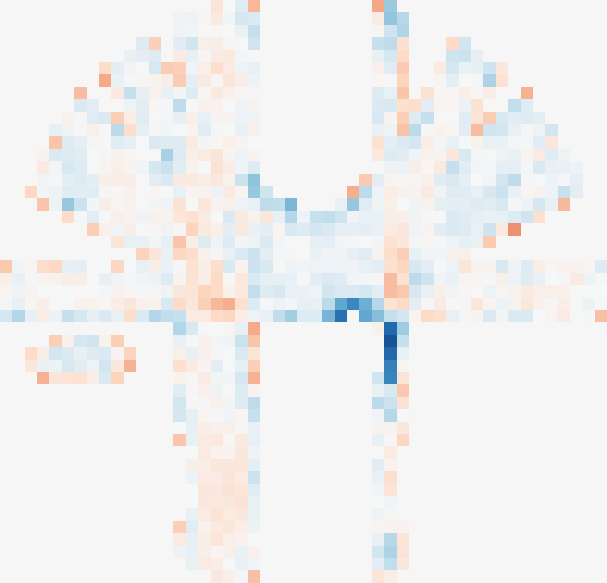
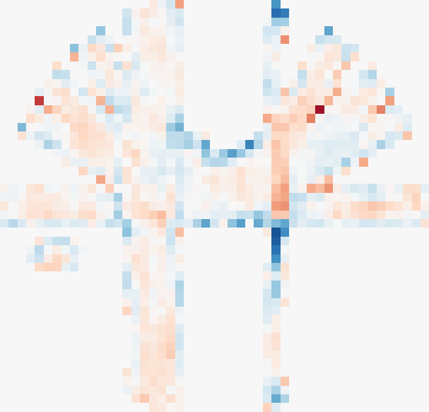
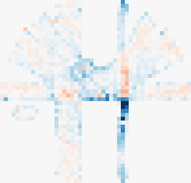
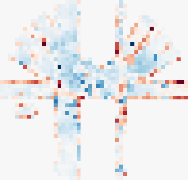
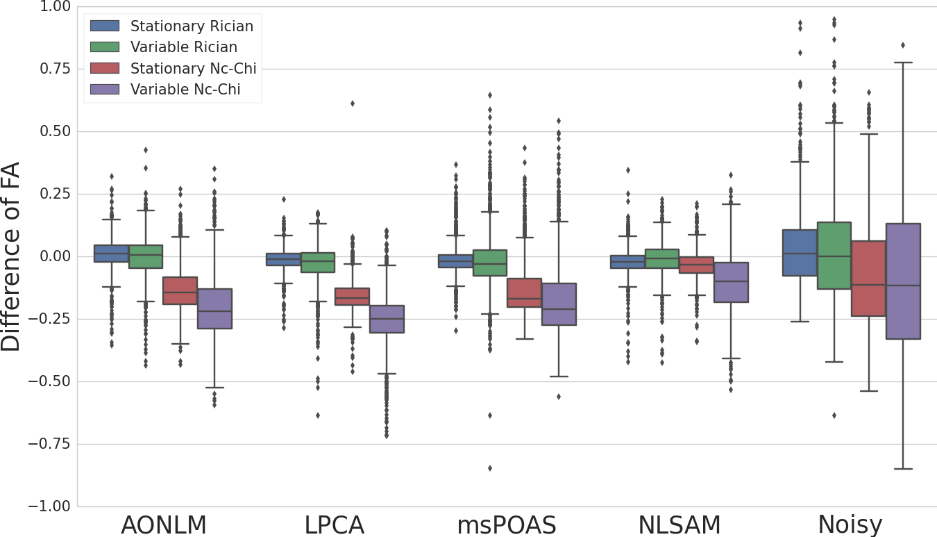
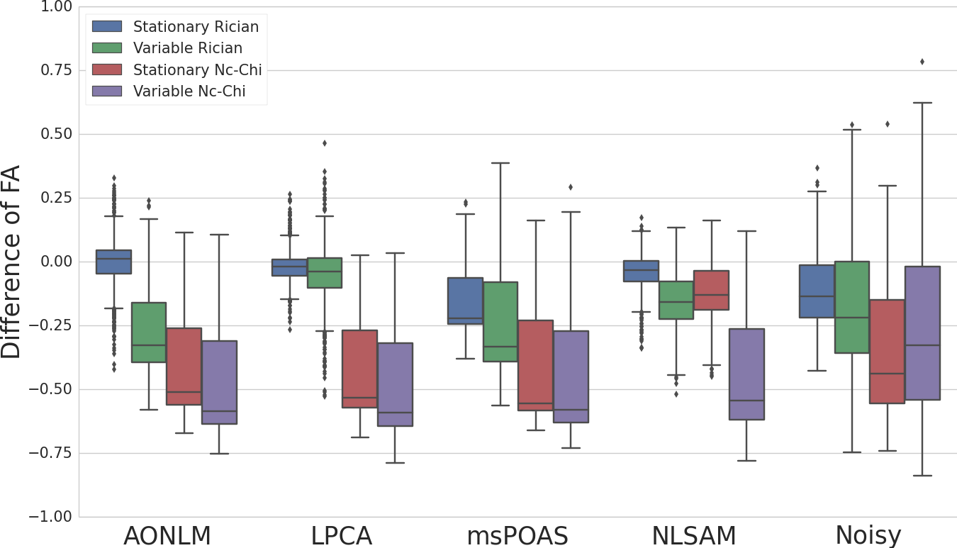
As shown by the FA difference map on Fig. 10, our NLSAM method commits a small FA error locally with a smaller maximum error than the compared methods. Voxelwise underestimation is denoted in blue and overestimation in red, where white means the computed value is close to the expected value. The noisy data largely overestimates the FA values for the synthetic datasets, while other denoising methods underestimate the real FA value most of the time. On the b1000 datasets, NLSAM has the smallest spread of FA error. The effect of stabilizing the data prior to denoising can also be seen by the stable FA median error committed by NLSAM across all noise types. For the b3000 datasets, the need to correct the intensity bias caused by the noise becomes more important, as seen by the increased error in underestimating the correct FA value for most methods. For the spatially varying Rician noise case, our method commits the lowest overestimation, as opposed to AONLM and LPCA, which are developed for this particular noise case. It is also important to note that in contrast to the other methods, msPOAS does not explicitly correct for the intensity bias by design, but rather leaves this correction to subsequent processing steps. The SNR 15 nc-$\chi$ noise case is where all the methods make the biggest error, as they reduce the variance but still suffer from a large bias in FA. Overall, our method restores the value of the FA for large bundles more accurately. We also see that most methods make their largest error near the partial volume ball mimicking cerebrospinal fluid (CSF).

Stationary nc-$\chi$

Spatially var. Rician

(a) Noisy

(b) NLSAM

(c) AONLM

(d) LPCA

(e) msPOAS

FA difference for the phantomas stationary nc-$\chi$ SNR 10 and spatially varying Rician SNR 15 b1000 datasets. Blue values denote underestimation while red values show overestimation of the FA. Top : Stationary nc-$\chi$ noise. NLSAM is less biased than the other methods in large, homogeneous regions, while the compared methods produces more underestimation for the nc-$\chi$ case. Bottom : Spatially variable Rician noise. While being a harder case than the SNR 10 dataset since it varies from SNR 5 to 15, all methods adapt themselves to some extent to the varying noise profile.

b1000

b3000

Figure 10: Boxplot of the difference in FA for the synthetic datasets at b1000 (left) and b3000 (right). The whiskers show 1.5 times the interquartile range (1.5 x IQR), where outliers are plotted individually. The bars represent the first quantile, the median and the third quartile. No method performs well on the nc-$\chi$ b3000 spatially varying noise case, which is the hardest test case. NLSAM overall produces less error or is equal to the other methods, but has a lower bias in the FA error along noise type.

4.3 Impact on angular and discrete number of compartments (DNC) error

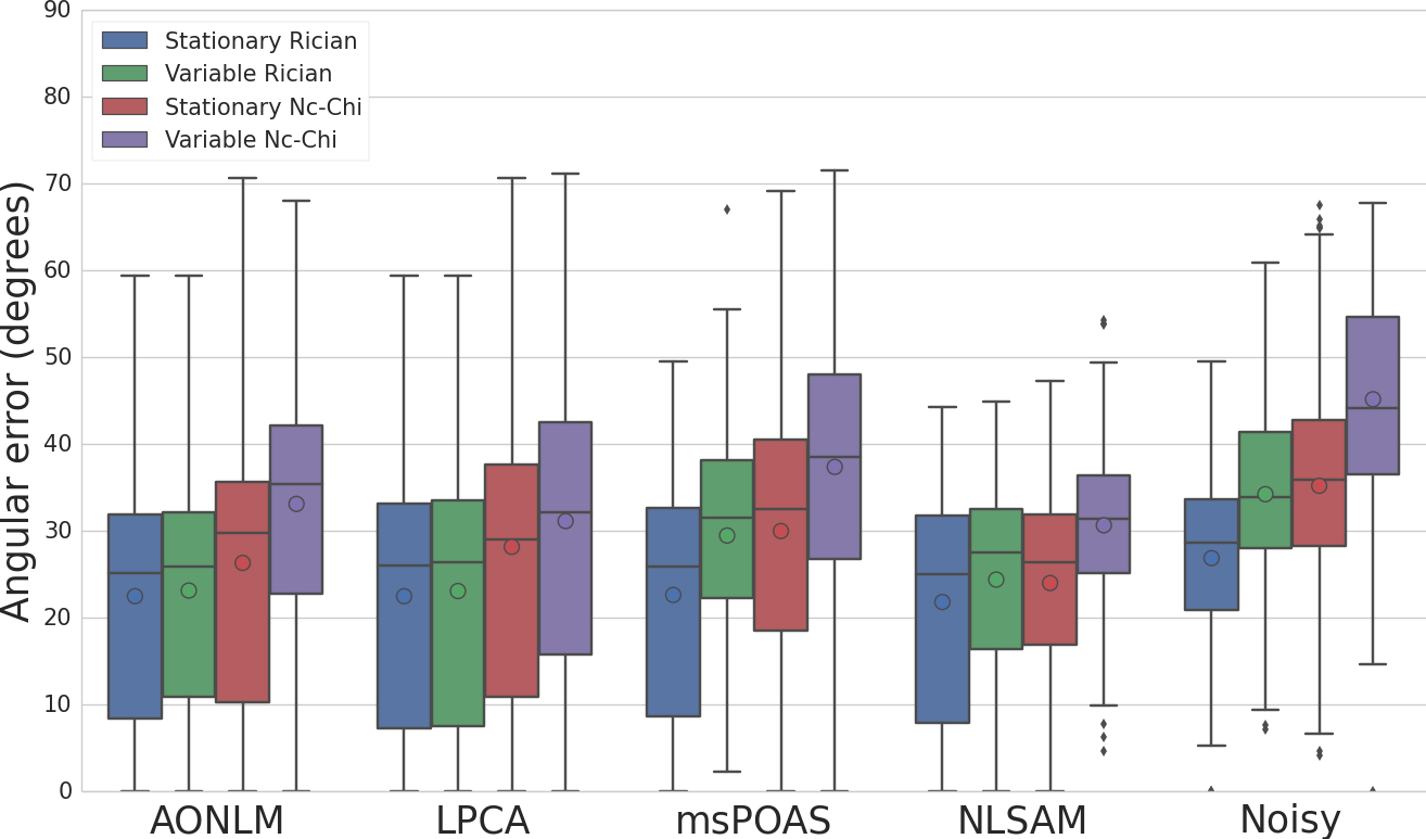
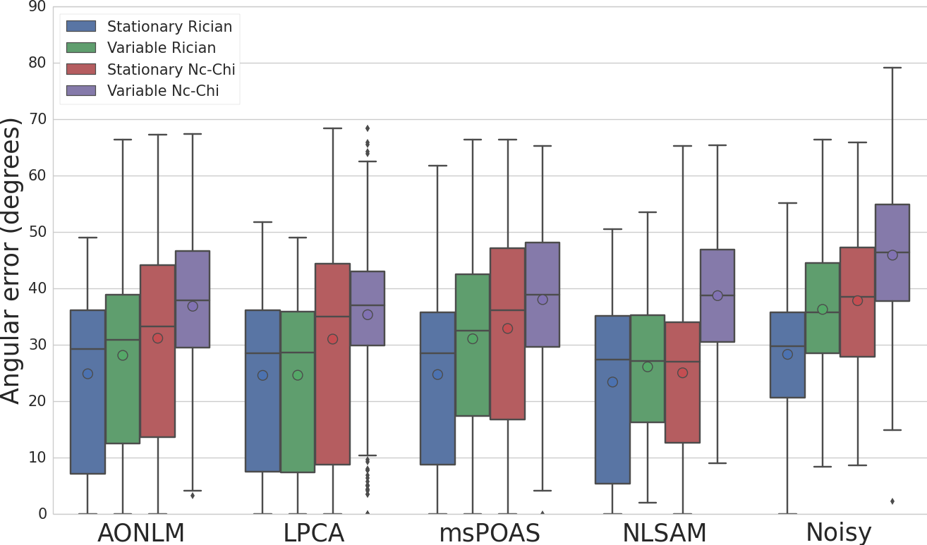
We now study the angular error and the mean relative error in the discrete number of compartments (DNC) (Paquette et al., 2014; Daducci et al., 2014). The mean relative discrete number of compartments error is defined as $DNC_{i}=100\times\lvert P_{i_{true}}-P_{i_{est}}\rvert/P_{i_{true}}$ for voxel $i$, $P_{i_{true}}$ and $P_{i_{est}}$ is the number of crossings respectively found on the noiseless dataset and on the compared dataset. All metrics were computed on the voxels containing at least two crossings fibers on the noiseless dataset shown previously in Fig. 5.

Fig. 12 shows the distribution of the angular error and of the DNC error found in the region studied in addition to the mean angular error. All of the denoising algorithms have a lower median and mean angular error than the noisy datasets. In addition, the NLSAM denoised datasets have an almost equal or lower angular error than the other denoising methods, but with a lower maximum error most of the time as shown by the smaller whiskers. For the b1000 dataset DNC error, all three of AONLM, LPCA and NLSAM improve on the noisy dataset for the Rician noise case as they are devised for this kind of data. LPCA also has a better performance than the other two for the spatially varying Rician noise case, while NLSAM has a lower mean DNC error for both of the nc-$\chi$ noise case. The effect of the intensity bias is also seen on msPOAS, where the DNC error is always lower than the noisy dataset, but also higher than all the other methods which take into account the intensity bias. The b3000 dataset is much harder, where no method seems to have a clear advantage in all cases over the others. One interesting thing to note is that the noisy dataset has a low DNC error for both of the Rician noise case, but the confidence interval indicates it is in the same range as the denoised datasets.

b1000

b3000

Boxplot of the angular error in degrees on the synthetic datasets, where the dot represents the mean angular error. A low angular error means that the extracted fODFs peaks are aligned with the noiseless dataset extracted peaks.

b1000

b3000

Figure 12: The mean relative percentage of DNC error for the synthetic datasets. The bar represents the 95% confidence interval on the mean as computed by bootstrapping. The DNC error is the number of peaks found in excess or missing in each voxel with respect to the noiseless dataset.

4.4 Impact on tractography

We now show how denoising techniques impact tractography by evaluating the number of valid bundles (VB), invalid bundles (IB) (Côté et al., 2013) and the valid connection to connection ratio (VCCR) (Girard et al., 2014) found by the tracking algorithm. A valid bundle is defined as connecting two ROIs in the ground truth data while an invalid bundle is a connection made between two ROIs which is not supported by the ground truth data. The valid connection to connection ratio is the total of valid connections (VC) over the sum of valid and invalid connections (IC), i.e. $VCCR=\frac{VC}{VC+IC}$. A good denoising algorithm should find a high number of valid bundles, a low number of invalid bundles and a high percentage of valid connection to connection ratio.

Deterministic tractography on the synthetic phantom

Table 2 shows the results of deterministic tractography on the SNR 10, 15 and 20 synthetic datasets for both b1000 and b3000. The noiseless b1000 dataset had 25/27 valid bundles, 55 invalid bundles and a valid connection to connection ratio of 65% and the noiseless b3000 dataset had 27/27 valid bundles, 40 invalid bundles and a valid connection to connection ratio of 68%. One of the first thing to note is that even though the noisy dataset always has a high number of valid bundles, it is at the price of a huge number of invalid bundles. Moreover, the valid connection to connection ratio is systematically lower for the SNR 10 datasets than any of the denoising methods. This indicates that only looking at the number of valid and invalid bundles does not show how many streamlines reached each region since only at least one streamline is required to make a connection, thus counting as a valid bundle. Another observation is that denoising helps controlling the number of invalid bundles and gives a better valid connection to connection ratio in most cases over the noisy data. For the SNR 15 cases, NLSAM has the highest number of valid bundles in almost all cases, but at the price of a larger number of invalid bundles at lower SNR. Another interesting trend is the tradeoff between valid bundles and invalid bundles : AONLM and LPCA both manage to get a lower number of invalid bundles, but also tend to have a lower number of valid bundles than msPOAS or NLSAM overall.

For the SNR 20 stationary noise cases, all methods are close in valid bundles with some difference in the number of invalid bundles. This shows that tractography could benefit from variable tracking parameters instead of fixed values depending on the preferred trade-off for the task at hand (Chamberland et al., 2014).

			Stationary noise						Spatially variable noise
			SNR 10			SNR 20			SNR 15			SNR 20
Method / Noise			VB	IB	VCCR	VB	IB	VCCR	VB	IB	VCCR	VB	IB	VCCR
AONLM	b1000	Rician	25	78	49%	25	75	51%	23	91	45%	25	89	50%
		nc-$\chi$	25	88	50%	26	88	52%	21	111	44%	23	93	47%
	b3000	Rician	25	69	52%	25	60	56%	24	85	50%	26	72	52%
		nc-$\chi$	25	78	55%	26	67	55%	20	95	48%	22	78	54%
LPCA	b1000	Rician	23	61	49%	25	64	54%	16	36	42%	18	38	45%
		nc-$\chi$	22	66	50%	24	70	54%	16	46	51%	20	56	52%
	b3000	Rician	23	44	47%	26	46	53%	17	37	42%	19	41	45%
		nc-$\chi$	20	42	58%	25	57	53%	18	40	55%	20	56	55%
msPOAS	b1000	Rician	25	101	49%	25	89	52%	23	129	44%	25	118	46%
		nc-$\chi$	23	121	40%	25	95	54%	20	131	35%	25	141	41%
	b3000	Rician	26	108	53%	26	74	58%	25	88	52%	25	93	49%
		nc-$\chi$	17	84	37%	25	84	57%	22	96	33%	23	94	47%
NLSAM	b1000	Rician	25	90	49%	26	96	54%	25	127	42%	25	114	45%
		nc-$\chi$	25	120	48%	25	90	54%	25	170	28%	26	144	43%
	b3000	Rician	25	92	50%	26	67	54%	25	108	43%	25	97	47%
		nc-$\chi$	23	100	45%	24	82	53%	23	173	29%	25	131	37%
Noisy	b1000	Rician	25	138	41%	25	107	53%	25	159	36%	25	134	42%
		nc-$\chi$	25	166	34%	26	119	49%	17	120	9%	25	209	24%
	b3000	Rician	25	116	46%	27	87	54%	25	160	36%	25	149	42%
		nc-$\chi$	25	182	36%	26	103	53%	18	124	9%	25	210	24%
Noiseless			VB		IC		VCCR
	b1000		25		55		65%
	b3000		27		40		68%

Table 2: Tractometer results for the deterministic tracking.

Tracking the real data

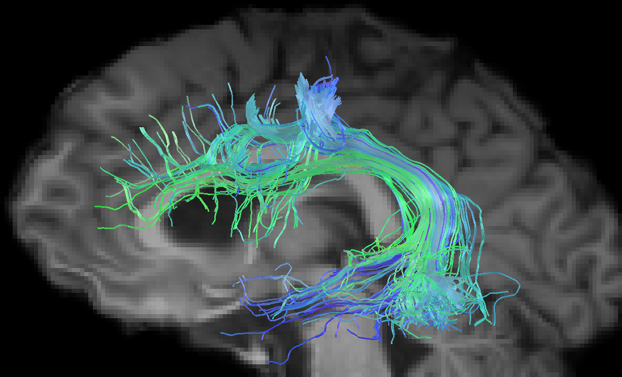
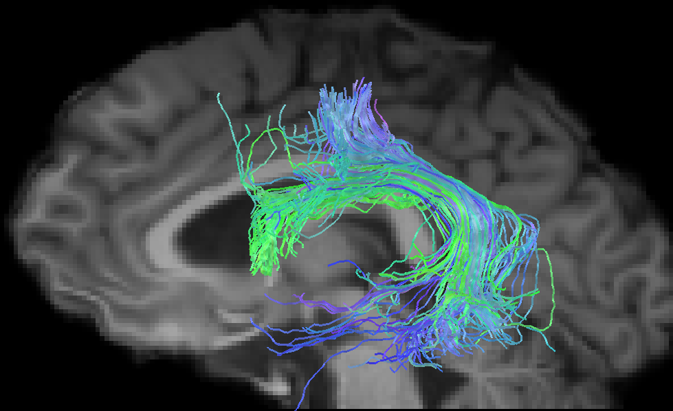
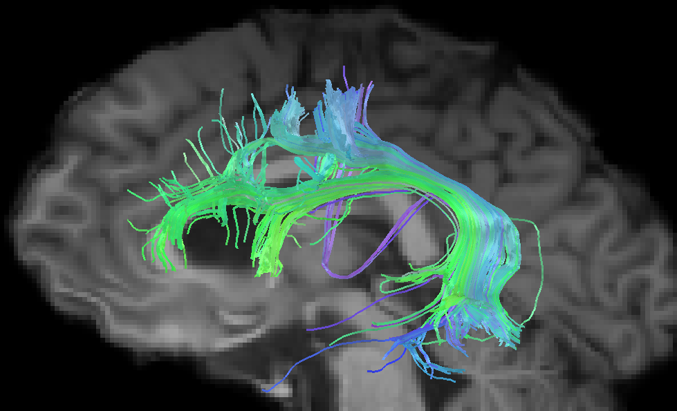
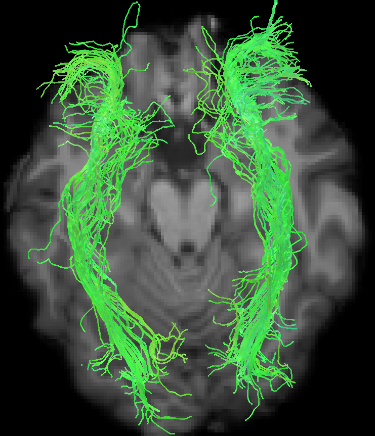
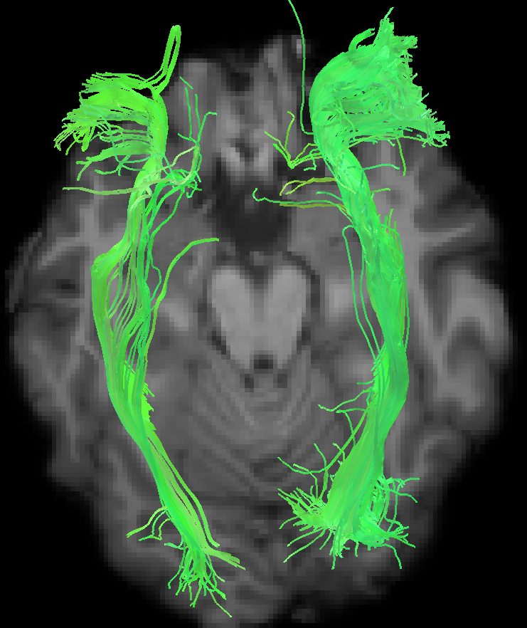
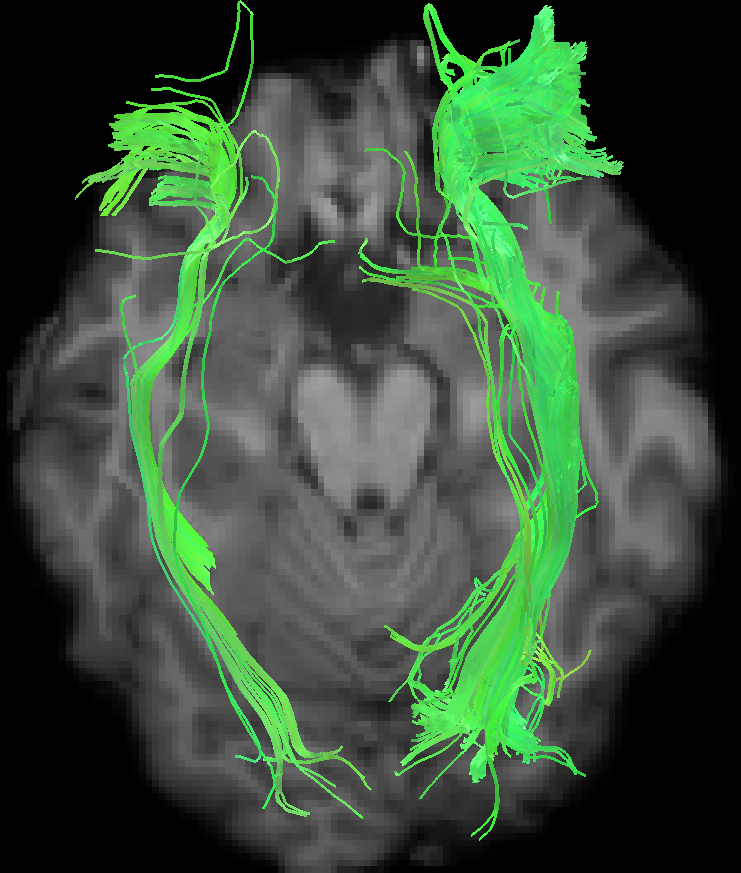
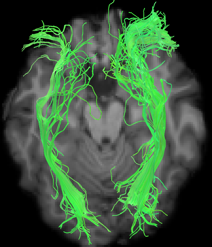
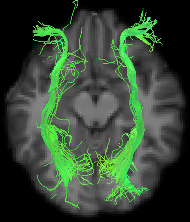
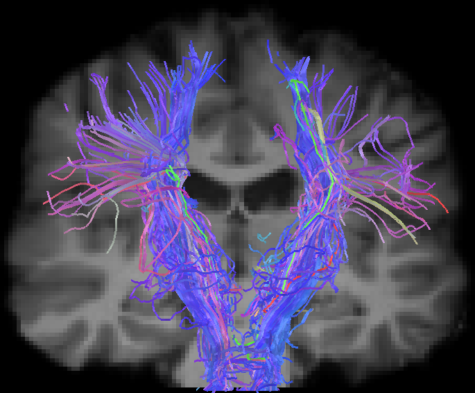
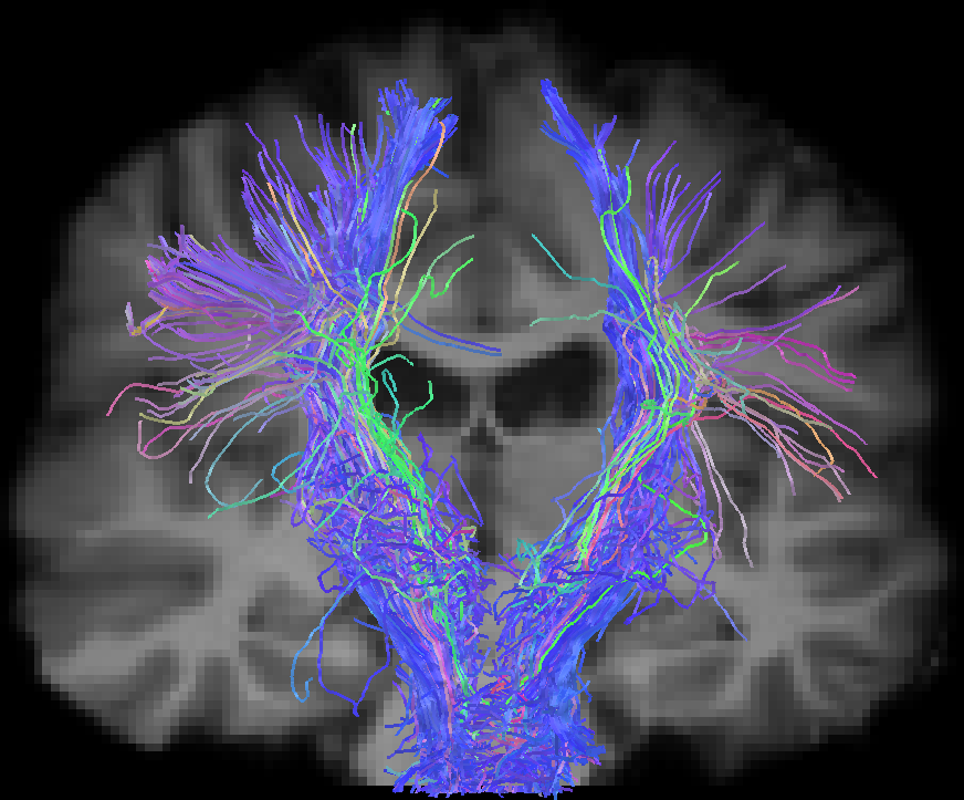
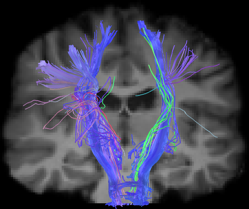
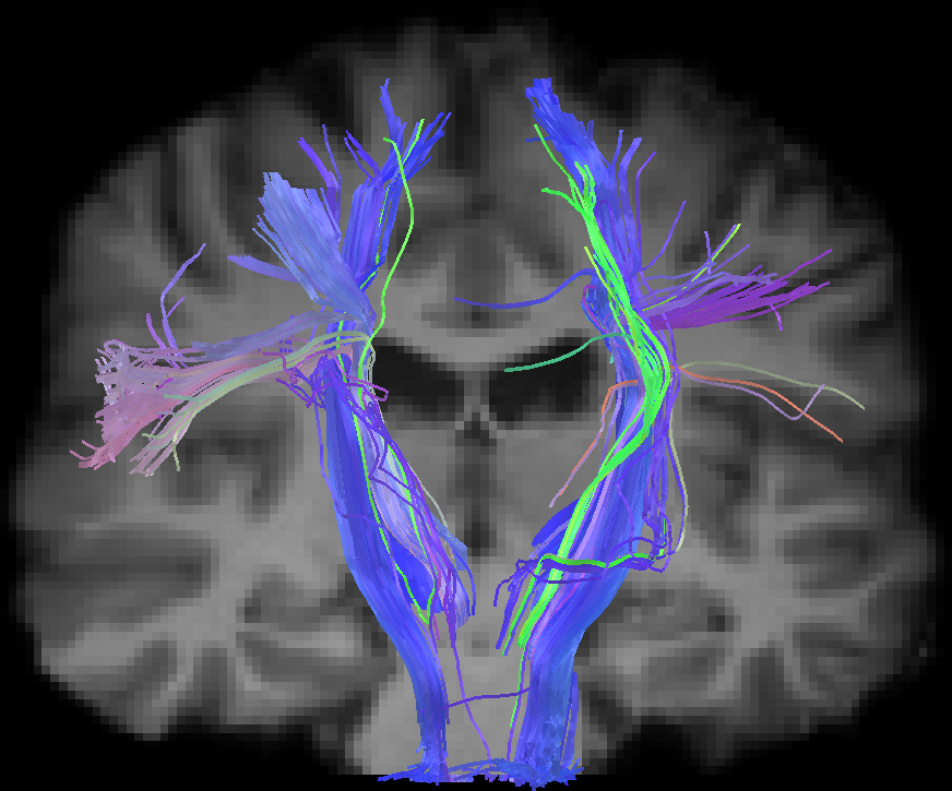
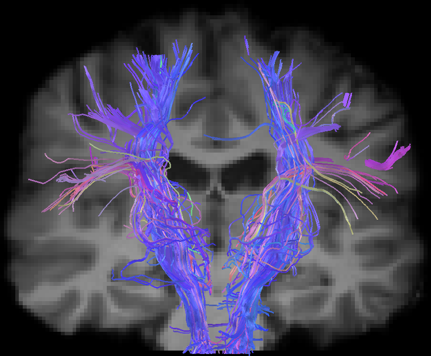
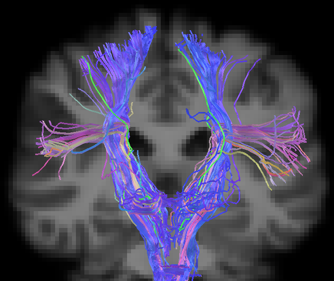
We now look at tractography on the in-vivo high spatial resolution dataset and its clinical spatial resolution counterpart of the same subject previously shown on Fig. 6. The high spatial resolution dataset at 1.2 mm isotropic has 40 unique gradient directions while the lower spatial resolution dataset at 1.8 mm isotropic has 64 unique gradient directions for a comparable acquisition time. The background is masked by the scanner and has a spatially varying Rician noise profile due to the SENSE reconstruction, which is the specific noise case covered by the AONLM and LPCA denoising algorithm. We use the deterministic tractography algorithm from (Girard et al., 2014), which considers anatomical constraints for more anatomically plausible tractography. Fig. 13 (which is displayed in landscape to present all the bundles at once) shows from top to bottom the left arcuate fasciculus (AF), the inferior fronto-occipital fasciculus (IFOF) and the corticospinal tract (CST) as dissected automatically by the Tract querier (Wassermann et al., 2013). The noisy 1.2 mm AF stops prematurely in the frontal part of the bundle, while the 1.8 mm noisy AF misses the temporal lobe. In contrast, the streamlines from the NLSAM denoised bundle go further into the temporal lobe. Also note how the right IFOF has a better coverage for all the 1.2 mm datasets and more fanning near the front of the brain than the noisy 1.8 mm dataset. We also see that the left IFOF is thinner than its right counterpart, but most of the bundles tracked from the denoised datasets produces less spurious tracks while keeping the anatomical details. The LPCA denoised IFOF stops prematurely for the left posterior part of the bundle, possibly because of a lost crossing region along the fibers during the denoising process. The CST does show some commissural fibers through the pons in the noisy 1.8 mm dataset, while they are present but look like spurious fibers on the noisy 1.2 mm dataset. AONLM can recover some of those commissural fibers, while NLSAM is the only algorithm which recovers them in addition to richer fanning near both sides of the motor cortex.

(a) NLSAM

(b) Noisy 1.2 mm

(c) AONLM

(d) LPCA

(e) msPOAS

(f) Noisy 1.8 mm

Figure 13: Deterministic tractography for selected bundles on the in-vivo dataset. We also show a T1 weighted image aligned in the diffusion space for anatomical reference. Top : The left arcuate fasciculus. Note how the denoised NLSAM arcuate fasciculus goes further into the frontal and temporal region than both of its noisy 1.2 mm and 1.8 mm counterparts. Middle : The inferior fronto-occipital fasciculus. The AONLM denoised bundle has a denser part for the right IFOF while the LPCA bundle stops prematurely for the left IFOF, possibly due to a missing crossing along the bundle. Bottom : The corticospinal tract. We see that NLSAM recovers the commissural fibers in the pons from the noisy 1.2 mm dataset, which are not even present on the noisy 1.8 mm dataset nor on the other denoising algorithm’s bundles. NLSAM also recovers more fanning to both sides of the brain than all the compared methods.

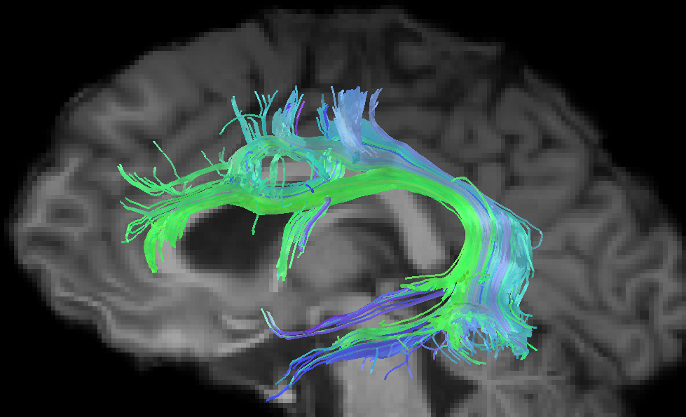
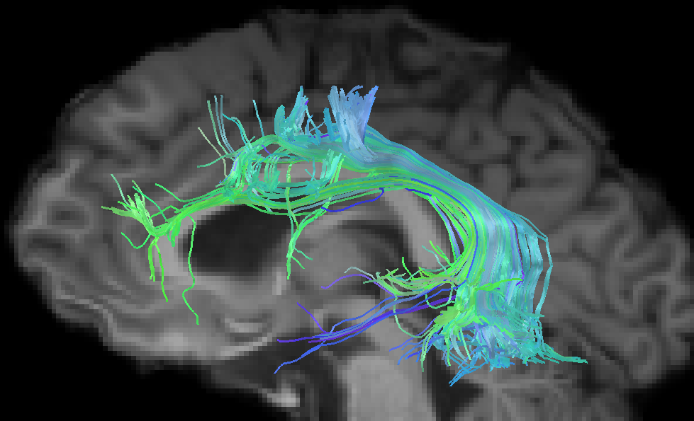
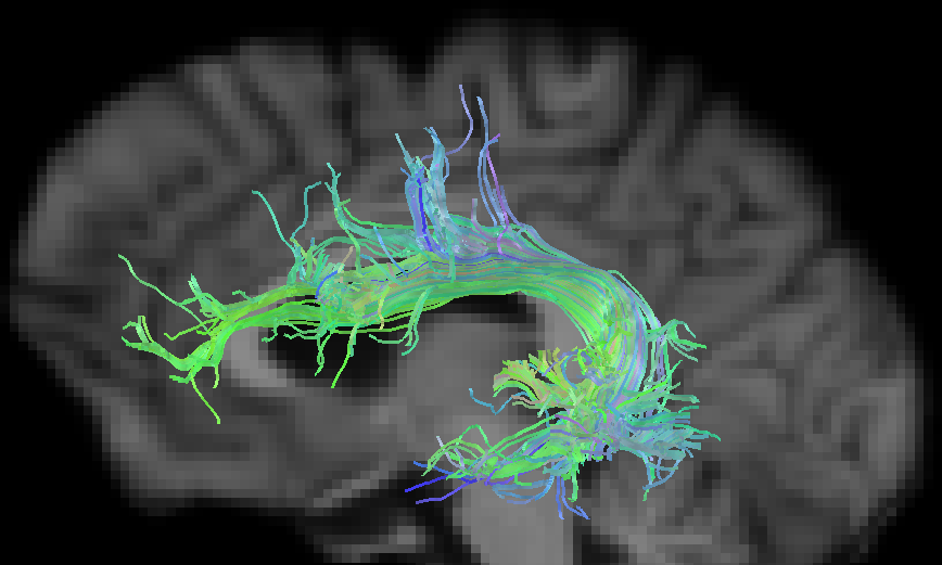
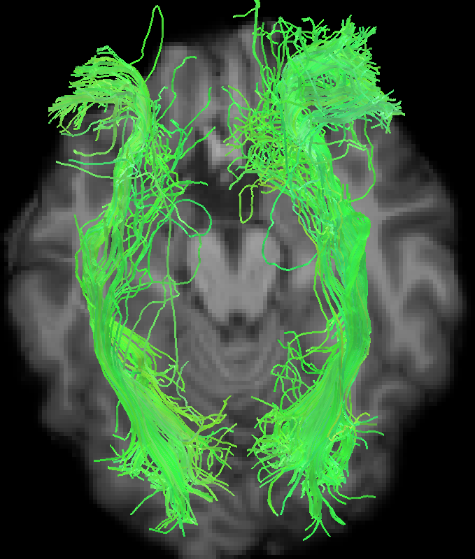
0

5 Discussion

5.1 Enhancing the raw data

We quantitatively showed in Fig. 7 that denoising restores perceptual information when compared to the unprocessed noisy data. Taking the spatially varying aspect and the particular nature of the noise into account is also important since modern scanners implement parallel imaging which changes the nature of the noise (Dietrich et al., 2008), leading to a lower performance for denoising methods not fully taking into account the introduced bias. Fig. 6 shows that this is also qualitatively true for in-vivo data, where denoising visually restores information in regions heavily corrupted by noise. While perceptual metrics might indicate the performance of an algorithm, one must remember that the relative signal difference is of interest in diffusion MRI, which is not fully captured by perceptual metrics like the PSNR or the SSIM. One is also usually interested in diffusion MRI metrics as opposed to perceptual information brought by the raw diffusion MRI datasets. AONLM is able to remove most of the noise, but still shows some residuals near the inferior part of the brain, possibly due to only considering the 3D volumes separately, which means that the algorithm can not benefit from the additional angular information brought by diffusion MRI. LPCA can restore visual information and sharp edges from the noisy dataset, but the region in the pons, where the noise level is higher and crossing fibers are more complex, also seems to be piecewise constant. This might arise from the fact that the algorithm uses all of the DWIs at once for its PCA decomposition step and treats all intensities at the same in the noise removal step. As for NLSAM, the algorithm only works in the local angular domain, thus exploiting similar contrast and redundant edge structure under different noise realization. msPOAS also uses a similar idea, where the angular similarity is weighted according to the Kullback-Leibler divergence to control the importance of dissimilar intensities in the denoising process. Nevertheless, these perceptual metrics show that denoising improves upon the noisy data, but one should also look at metrics derived from the studied object of interest i.e. tensor or fODF derived metrics, since high perceptual metrics might also reflect blurring of diffusion features, which is the main interest in this type of acquisition rather than the perceived quality.

5.2 Impact of the stabilization algorithm on the compared denoising methods

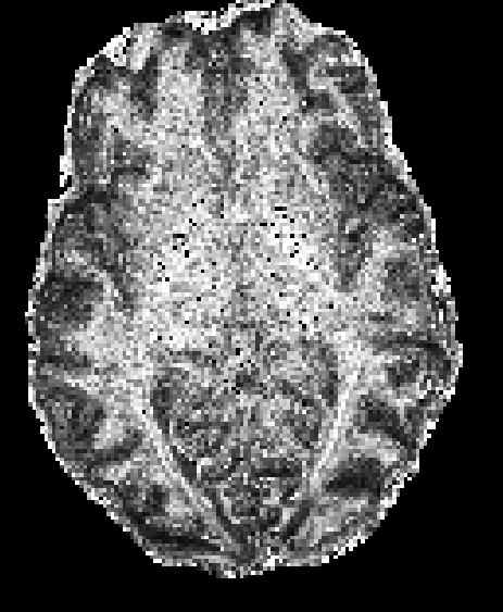
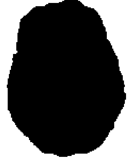
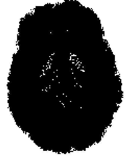
Fig. 14 shows the FA map when the compared denoising algorithm are applied on the stabilized data with the algorithm of (Koay et al., 2009a). For this experiment, we consider a voxel as being degenerated if its FA is exactly 0. The first thing to note is that the algorithm only reprojects the noisy data on plausible Gaussian distributed values and does not do any denoising. While we used here the algorithm of (Koay et al., 2009a) to correct the noise bias, another interesting approach consist of producing real-valued datasets as shown in (Eichner et al., 2015). This approach does not require estimation of $\sigma^{2}$ or $N$, but instead use information contained in the phase of complex-valued acquisitions. Secondly, all of the other compared denoising algorithms produce some invalid voxels on the raw dataset, while having less degenerated voxels on the stabilized dataset as shown in Table 3. Nevertheless, only our NLSAM algorithm does not produce any degenerated FA voxel on the in-vivo dataset. As tractography might rely on a thresholded FA mask (Chamberland et al., 2014), any missing white matter voxel will end the tractography early and produce anatomically invalid tractography. In the same way, computing FA based statistics in search of group differences inside a white matter mask might lead to erroneous conclusions when degenerated voxels are present. This undesirable side effect should be avoided when possible by choosing a method producing a low number of invalid voxels, such as NLSAM.

(a) Noisy

(b) NLSAM

(c) AONLM

(d) LPCA

(e) msPOAS

Figure 14: Effect of the stabilization algorithm on the compared methods. The top row shows an axial slice of the in-vivo FA map computed on the stabilized dataset, where some voxels are degenerated. The bottom row shows their location on a binary brain mask. As shown in Table 3, all methods produce degenerated FA voxels on both the regular and stabilized data, with the sole exception of NLSAM.

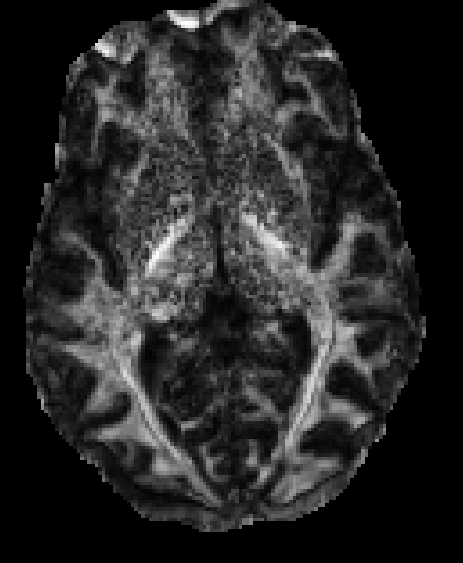
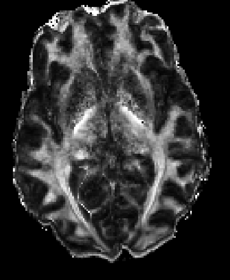
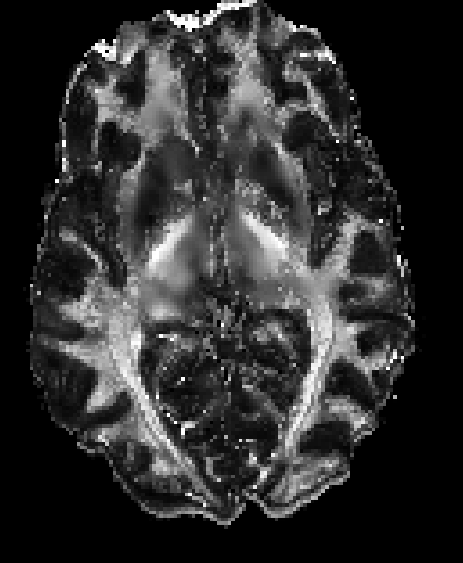
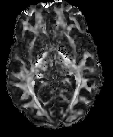
		AONLM	LPCA	msPOAS	NLSAM	Noisy	Mask
Built-in	Brain mask	83 314 (10.1%)	10 526 (1.3%)	84 319 (10.2%)	$\oslash$	5 994 (0.7%)	823 068 (100%)
	WM mask	29 664 (5.1%)	1 298 (0.2%)	16 665 (2.9%)	$\oslash$	1 769 (0.3%)	578 418 (100%)
Stabilization	Brain mask	10 052 (1.2%)	15 750 (1.9%)	29 377 (3.6%)	0 (0%)	9 395 (3.6%)	823 068 (100%)
	WM mask	404 (0.1%)	1 468 (0.3%)	4 267 (0.7%)	0 (0%)	2 850 (0.5%)	578 418 (100%)

Table 3: Number of degenerated FA voxels inside a brain mask and a white matter mask for the in-vivo dataset. All methods were compared with their built-in noise estimation on the stabilized version, but without any additional noise correction factor. The percentage of degenerated voxels is indicated in parenthesis for each mask, where a voxel is considered degenerated if its FA value is exactly 0.

5.3 Reducing the diffusion metrics bias

Fig. 10 shows that knowing where errors are committed gives a better view of how denoising improves upon the noisy data. We see that our NLSAM algorithm actually has a smaller maximum error in underestimating the FA most of the time while other methods both over and underestimate the real FA value and make larger errors near CSF or at borders with the background. This could indicate that they are subject to problems with partial volume effect, which seems less important for NLSAM.

While stabilizing the data alleviates the FA underestimation problem in most cases, it also helps to reduce the number of degenerated voxels in the in-vivo data as shown in Fig. 14. Both AONLM and msPOAS produce less degenerated FA voxels on the stabilized dataset as shown in Table 3, while NLSAM does not produce any degenerated voxel. In contrast, the noisy data and LPCA have an increased number of degenerated FA voxels, which might be caused by the diffusion signal being near the noise floor, thus producing a flat profile which is not properly recovered in this case. Reducing the FA bias and avoiding degenerated voxels by including denoising in the processing pipeline could improve the statistical analysis in along-tract metrics (Colby et al., 2012) when looking for group differences.

5.4 Restoring the coherence of local models

The CSD algorithm relies on the estimation of the fiber response function (frf), which in turn relies on the diffusion tensor. To estimate the frf, one must select voxels containing only a single fiber population. One way to do this is to estimate it from voxels with a high FA, usually with FA > 0.7 (Tournier et al., 2007; Descoteaux et al., 2009). We observed that for the SNR 10 dataset with nc-$\chi$ noise, the noisy dataset, AONLM and LPCA could not find as much single fiber voxels based on the FA threshold method as msPOAS or NLSAM since their reconstructed tensors have an inherently lower FA. This in turns impacts deconvolution since the estimates used for the deconvolution kernel are less stable, and lowering the FA threshold too much might violates the single fiber assumption, which is crucial for the CSD algorithm. One way to circumvent this could be by using the method of (Tax et al., 2014), which is based on a peak amplitude criterion instead of an FA threshold to identify single fiber voxels.

Fig. 12 shows that msPOAS and NLSAM have larger angular error than AONLM or LPCA, but this does not seem to impact much the number of valid bundles found by deterministic tractography. Indeed, the noisy data has the largest angular error in all cases, but still has a high number of valid bundles in most cases. This also suggests that a large overestimation or underestimation of fiber crossings (as reflected by the DNC error) has a higher impact on tractography. Both LPCA and msPOAS have a lower number of valid bundles than AONLM or NLSAM, which both have a rather symmetric under and over estimation of the number of peaks. This means that an overall estimation or underestimation of the number of crossings bias tractography, as it tends to follow false crossings or stops prematurely due to a lack of crossings, while a distributed error is not skewed toward these effects.

In Fig. 6, we see that denoising restores coherence in regions of crossing fibers that were lost on the noisy dataset or not even present in the lower spatial resolution 1.8 mm dataset due to a smaller voxel size. We also see that NLSAM restores more coherent crossings than the other denoising methods in the junction of the SLF and the CST, whereas the noisy dataset only shows incoherent crossings. This actually enables tractography algorithms to reconstructs tracts which are in agreement with the expected anatomy. In the same amount of acquisition time, one can thus acquire higher spatial resolution DWIs and get better angular information by post-processing the acquired data with denoising.

5.5 Limiting spurious fibers from tractography

We studied the impact of denoising techniques on deterministic tractography on a synthetic dataset in Section 4.4. One often has to choose between having a high number of valid bundles and invalid bundles, or having less valid bundles and at the same time reducing the amount of invalid bundles. The noisy dataset always reaches a high number of valid bundles, but also at the price of having the highest number of invalid bundles most of the time. Our NLSAM algorithm shows a good balance between the number of valid and invalid bundles at low SNR, especially for the spatially varying noise case. This is always a tradeoff that one has to choose as seen in the ISMRM 2015 tractography challenge.

For example, the LPCA algorithm has always a low number of invalid bundles, but also the lowest number of valid bundles for the spatially varying noise case. In opposition, NLSAM has a high number of valid bundles, but also a high number of invalid bundles most of the time.

Regarding the deterministic tractography, changing the stepsize or the maximum curving angle would give different results in terms of connectivity metrics, indicating that the tractography algorithm and chosen tractography parameters have a non negligible influence on the end results (Chamberland et al., 2014; Girard et al., 2014). We also used a seeding strategy of 100 seeds per voxel from the ROIs at each bundles endpoints to ensure a maximal number of valid bundles, which promotes a high number of valid bundles for each dataset. This shows that the missed bundles are hard to recover or not supported by the data itself, as opposed to being missed because of inadequate seeding (Côté et al., 2013). On the other hand, this can artificially increase the number of invalid bundles, which could be reduced by reducing the number of seeds per voxel. Since automatic tractography pruning techniques such as (Côté et al., 2015) might help reduce the number of spurious tracks, this would indicate that having a higher number of valid bundles would be preferable since invalid bundles could be potentially removed afterward. In contrast, a low number of valid bundles cannot be circumvented with further postprocessing. Nevertheless, denoising increases the valid connection to connection ratio and reduces the number of invalid bundles, thus bringing confidence in the validity of the tractography results when compared to the noisy datasets.

For the in-vivo dataset tracking shown in Fig. 13, we see that tractography benefits from higher spatial resolution acquisitions, but that the produced tracts are slightly more noisy. Combining the high spatial resolution, highly noisy dataset with a denoising algorithm at the beginning of the processing pipeline gives more anatomically plausible tracts in the end. The AF and CST produced by the NLSAM denoised dataset are both more anatomically plausible than their noisy or lower spatial resolution counterpart, which have less fanning fibers in the case of the CST. This shows that high resolution DWIs exhibits more anatomical information thanks to the smaller voxel size which might not be easily discernible at a lower spatial resolution (Sotiropoulos et al., 2013). Acquiring at higher spatial resolution could also help resolve complicated fiber configurations such as crossings fibers from fanning fibers or disentangle small structures like the optic chiasm (Roebroeck et al., 2008), which is not possible at lower spatial resolution (Jones et al., 2013; Calabrese et al., 2014).

5.6 Other methods for high spatial resolution acquisitions

We have shown in Fig. 6 that high spatial resolution acquisitions which are noisy at first can reveal improved anatomical details when they are subsequently denoised. This indeed suggests that high resolution acquisition can now be acquired on clinical scanners. Recently, other algorithms enabling a high spatial resolution at the acquisition level have been suggested (Scherrer et al., 2015; Ning et al., 2016). These methods both rely on smartly fusing the (complementary) data of multiple acquisitions acquired at a lower spatial resolution to obtain a single high resolution volume. While the approach we suggest here is to acquire a single volume using a standard sequence, both techniques are fundamentally exploiting different aspects to increase the available spatial resolution. As such, it would be possible to combine our denoising algorithm with the reconstruction algorithms presented in (Scherrer et al., 2015; Ning et al., 2016).

5.7 Current limitations and possible improvements

Although most models assume a Rician or nc-$\chi$ noise distribution, this does not take into account the noise correlation between each coils or the effect of acceleration techniques that subsample the k-space (Aja-Fernández et al., 2014). The development of correction factors for existing algorithms relies on computing the effective values for the noise standard deviation $\sigma$ and the number of degrees of freedom of the nc-$\chi$ distribution, which is expected to be smaller than 2N. These values can be used to take into account the correlation introduced between the coils in parallel imaging acquisitions (Brion et al., 2013). To consider the fact that the noise distribution nature might vary spatially in addition to the noise variance, one can use a priori information obtained from the scanner through the SENSE sensitivity maps or the GRAPPA weights and need to estimate the correlation between each of the receiver coils. We could explicitly add such a correction to our algorithm since we work locally with the stabilization algorithm, Eq. (1) and Eq. (4). Using multiband acceleration also modifies the noise properties due to the introduced aliasing, which further strengthen the idea that spatially adaptive denoising algorithms should be used on modern scanners and sequences (Ugurbil et al., 2013). Nevertheless, obtaining the needed map for a SENSE reconstruction or the required GRAPPA weights might not be easily feasible in a clinical setting. We also intend to revisit the order in which preprocessing algorithms (motion correction, eddy currents correction, distortions correction) should be applied since these steps require interpolation, which could also introduce spatial correlation in the noise profile. This also makes the noise distribution deviate slightly from its theoretical distribution, where parameters vary spatially instead of being fixed constants for the whole volume (Aja-Fernández et al., 2014). Nevertheless, we have observed experimentally that our NLSAM algorithm is robust to small subject motion thanks to the local neighborhood processing. In case where artifacts (such as epi distortions) might undermine the denoising process, one can first correct for these artifacts using a nearest neighbor interpolation, which should not modify the noise distribution. Subsequent corrections can then be performed after denoising using other kinds of interpolation as needed.

While developing the NLSAM algorithm, we found that using a bigger 3D patchsize did not significantly improve the denoising quality, while augmenting both computing time and memory requirements. Our implementation also allows one create the smallest subset of angular neighbors covering all DWIs through a greedy set cover algorithm. This option (named "NLSAM fast" in Table 4) leads to a speedup of 3 to 4 times, but at the cost of slightly reducing the denoising performance since some DWIs might be denoised only once instead of multiple times. We used the fully covered version for our experiments, which were run on a machine running Ubuntu Linux 12.04 with a quad core Intel i7 930 at 2.8 GHz and 18 GB of RAM. Table 4 reports the runtime of the various algorithms in minutes and their RAM usage. While the computing time required by NLSAM is larger than the other methods, our Python implementation is fairly unoptimized and could be sped up to competitive runtimes by various code optimizations or lowering the maximum number of iterations in Eq. (4).

	AONLM	LPCA	msPOAS	NLSAM	NLSAM fast
Time (mins)	22.2	3.7	4.0	37.1	9.8
RAM usage (MB)	552	640	1543	606	412

Table 4: Required time and RAM usage for the compared denoising algorithms on the b1000 SNR 10 dataset with stationary Rician noise.

6 Conclusion

In this paper, we introduced a new denoising method, the Non Local Spatial and Angular Matching (NLSAM), which is specifically designed to take advantage of diffusion MRI data. Our method is based on 1) Correcting the spatially varying Rician and nc-$\chi$ noise bias 2) Finding similar DWIs through angular neighbors to promote sparsity 3) Iteratively denoise similar patches and their neighbors locally with dictionary learning, where the local variance is used as an upper bound on the $\ell_{2}$ reconstruction error. We extensively compared quantitatively our new method against three other state-of-the-art denoising methods on a synthetic phantom and qualitatively on an in-vivo high resolution dataset. We also showed that taking into account both the effect of spatially varying noise and non-Gaussian distributed noise is crucial in order to denoise effectively the DWIs. Our NLSAM algorithm is freely available, restores perceptual information, removes the noise bias in common diffusion metrics and produces more anatomically plausible tractography on a high spatial resolution in-vivo dataset when compared to a lower spatial resolution acquisition of the same subject.

Since our NLSAM algorithm can be used on any already acquired dataset and does not add any acquisition time, this shows that denoising the data should be a pre-processing part of every pipeline, just like any other correction method that is commonly applied for artifacts removal. With that in mind, the diffusion MRI community could aim for higher spatial resolution DWIs, without requiring the use of costly new hardware or complicated acquisition schemes. This could in turn reveal new anatomical details, which are not achievable at the spatial resolution currently used in diffusion MRI.

Appendix A The NLSAM Algorithm

This appendix outlines the NLSAM algorithm as pseudo code. The original implementation in Python is freely available at https://github.com/samuelstjean/nlsam.

Data: 4D dMRI data, $an=$ number of angular neighbors, $ps=$ spatial patch size, $N=$ Number of coils, $max\_iter=40$

Result: Denoised data with NLSAM

Step 1;

          Find $\sigma_{G}$ with either PIESNO or Eq. (3);

          Apply noise stabilization with $\sigma_{G}$ and $N$ coils;

foreach DWI in dMRI data do

       Step 2;

                 Find the closest $an$ angular neighbors;

                 Create 4D block with b0, DWI and its $an$ neighbors;

                 Extract all overlapping patches of size $(ps,ps,ps)$;

      

      Step 3;

                 Apply Eq. (1) to find D;

                 Iterate Eq. (4) to find $\boldsymbol{\alpha}$ until convergence or $max\_iter$ is reached;

                 Average overlapping patches based on sparsity with Eq. (5);

                 Return to original shape;

      

end foreach

foreach Denoised DWI in dMRI data do

       Average all Denoised DWI representations;

      

end foreach

Algorithm 1 The proposed NLSAM denoising algorithm.

References

- Aja-Fernandez et al. (2008) Aja-Fernandez, S., Alberola-Lopez, C., Westin, C.F., 2008. Noise and signal estimation in magnitude MRI and Rician distributed images: a LMMSE approach. IEEE transactions on image processing 17, 1383–98.
- Aja-Fernández et al. (2014) Aja-Fernández, S., Vegas-Sánchez-Ferrero, G., Tristán-Vega, A., 2014. Noise estimation in parallel MRI: GRAPPA and SENSE. Magnetic resonance imaging 32, 281–90.
- Alexander et al. (2010) Alexander, D.C., Hubbard, P.L., Hall, M.G., Moore, E.a., Ptito, M., Parker, G.J.M., Dyrby, T.B., 2010. Orientationally invariant indices of axon diameter and density from diffusion MRI. NeuroImage 52, 1374–1389.
- Bai et al. (2014) Bai, R., Koay, C.G., Hutchinson, E., Basser, P.J., 2014. A framework for accurate determination of the T2 distribution from multiple echo magnitude MRI images. Journal of Magnetic Resonance 244, 53–63.
- Bao et al. (2013) Bao, L., Robini, M., Liu, W., Zhu, Y., 2013. Structure-adaptive sparse denoising for diffusion-tensor MRI. Medical image analysis 17, 442–57.
- Becker et al. (2014) Becker, S., Tabelow, K., Mohammadi, S., Weiskopf, N., Polzehl, J., 2014. Adaptive smoothing of multi-shell diffusion weighted magnetic resonance data by msPOAS. NeuroImage .
- Brion et al. (2013) Brion, V., Poupon, C., Riff, O., Aja-Fernández, S., Tristán-Vega, A., Mangin, J.F., Le Bihan, D., Poupon, F., 2013. Noise correction for HARDI and HYDI data obtained with multi-channel coils and sum of squares reconstruction: an anisotropic extension of the LMMSE. Magnetic resonance imaging 31, 1360–71.
- Calabrese et al. (2014) Calabrese, E., Badea, A., Coe, C.L., Lubach, G.R., Styner, M.A., Johnson, G.A., 2014. Investigating the tradeoffs between spatial resolution and diffusion sampling for brain mapping with diffusion tractography: Time well spent? Human Brain Mapping .
- Candès et al. (2008) Candès, E.J., Wakin, M.B., Boyd, S.P., 2008. Enhancing sparsity by reweighted l1 minimization. Journal of Fourier Analysis and Applications 14, 877–905.
- Chamberland et al. (2014) Chamberland, M., Whittingstall, K., Fortin, D., Mathieu, D., Descoteaux, M., 2014. Real-time multi-peak tractography for instantaneous connectivity display. Frontiers in neuroinformatics 8, 59.
- Colby et al. (2012) Colby, J.B., Soderberg, L., Lebel, C., Dinov, I.D., Thompson, P.M., Sowell, E.R., 2012. Along-tract statistics allow for enhanced tractography analysis. NeuroImage 59, 3227–3242.
- Côté et al. (2015) Côté, M.A., Garyfallidis, E., Larochelle, H., Descoteaux, M., 2015. Cleaning up the mess: tractography outlier removal using hierarchical QuickBundles clustering, in: Proceedings of: International Society of Magnetic Resonance in Medicine (ISMRM).
- Côté et al. (2013) Côté, M.A., Girard, G., Boré, A., Garyfallidis, E., Houde, J.C., Descoteaux, M., 2013. Tractometer: Towards validation of tractography pipelines. Medical image analysis 17.
- Coupé et al. (2008) Coupé, P., Yger, P., Prima, S., Hellier, P., Kervrann, C., Barillot, C., 2008. An optimized blockwise nonlocal means denoising filter for 3-D magnetic resonance images. IEEE transactions on medical imaging 27, 425–41.
- Dabov et al. (2007) Dabov, K., Foi, A., Katkovnik, V., Egiazarian, K., 2007. Image denoising by sparse 3-D transform-domain collaborative filtering. IEEE transactions on image processing 16, 2080–95.
- Daducci et al. (2014) Daducci, A., Canales-Rodríguez, E.J., Descoteaux, M., Garyfallidis, E., Gur, Y., Lin, Y.C., Mani, M., Merlet, S., Paquette, M., Ramirez-Manzanares, A., Reisert, M., Reis Rodrigues, P., Sepehrband, F., Caruyer, E., Choupan, J., Deriche, R., Jacob, M., Menegaz, G., Prčkovska, V., Rivera, M., Wiaux, Y., Thiran, J.P., 2014. Quantitative comparison of reconstruction methods for intra-voxel fiber recovery from diffusion MRI. IEEE transactions on medical imaging 33, 384–99.
- Daubechies et al. (2010) Daubechies, I., Devore, R., Fornasier, M., Güntürk, C.S., 2010. Iteratively reweighted least squares minimization for sparse recovery. Communications on Pure and Applied Mathematics 63, 1–38.
- Descoteaux et al. (2009) Descoteaux, M., Deriche, R., Knösche, T.R., Anwander, A., 2009. Deterministic and probabilistic tractography based on complex fibre orientation distributions. IEEE transactions on medical imaging 28, 269–86.
- Descoteaux and Poupon (2014) Descoteaux, M., Poupon, C., 2014. Diffusion-Weighted Imaging, in: Belvic, D., Belvic, K. (Eds.), Comprehensive Biomedical Physics.
- Dietrich et al. (2008) Dietrich, O., Raya, J.G., Reeder, S.B., Ingrisch, M., Reiser, M.F., Schoenberg, S.O., 2008. Influence of multichannel combination, parallel imaging and other reconstruction techniques on MRI noise characteristics. Magnetic resonance imaging 26, 754–62.
- Eichner et al. (2015) Eichner, C., Cauley, S.F., Cohen-Adad, J., Möller, H.E., Turner, R., Setsompop, K., Wald, L.L., 2015. Real diffusion-weighted MRI enabling true signal averaging and increased diffusion contrast. NeuroImage .
- Elad and Aharon (2006) Elad, M., Aharon, M., 2006. Image denoising via sparse and redundant representations over learned dictionaries. IEEE transactions on image processing 15, 3736–45.
- Foi (2011) Foi, A., 2011. Noise estimation and removal in MR imaging: The variance-stabilization approach. 2011 IEEE International Symposium on Biomedical Imaging: From Nano to Macro , 1809–1814.
- Garyfallidis et al. (2014) Garyfallidis, E., Brett, M., Amirbekian, B., Rokem, A., Van Der Walt, S., Descoteaux, M., Nimmo-Smith, I., 2014. Dipy, a library for the analysis of diffusion MRI data. Frontiers in Neuroinformatics 8.
- Girard et al. (2014) Girard, G., Whittingstall, K., Deriche, R., Descoteaux, M., 2014. Towards quantitative connectivity analysis: reducing tractography biases. NeuroImage 98, 266–78.
- Gramfort et al. (2014) Gramfort, A., Poupon, C., Descoteaux, M., 2014. Denoising and fast diffusion imaging with physically constrained sparse dictionary learning. Medical image analysis 18, 36–49.
- Jones et al. (2013) Jones, D.K., Knösche, T.R., Turner, R., 2013. White Matter Integrity, Fiber Count, and Other Fallacies: The Do’s and Don’ts of Diffusion MRI. NeuroImage 73, 239–254.
- Koay and Basser (2006) Koay, C.G., Basser, P.J., 2006. Analytically exact correction scheme for signal extraction from noisy magnitude MR signals. Journal of magnetic resonance 179, 317–22.
- Koay et al. (2009a) Koay, C.G., Ozarslan, E., Basser, P.J., 2009a. A signal transformational framework for breaking the noise floor and its applications in MRI. Journal of magnetic resonance 197.
- Koay et al. (2009b) Koay, C.G., Ozarslan, E., Pierpaoli, C., 2009b. Probabilistic Identification and Estimation of Noise (PIESNO): a self-consistent approach and its applications in MRI. Journal of magnetic resonance (San Diego, Calif. : 1997) 199, 94–103.
- Lam et al. (2014) Lam, F., Babacan, S.D., Haldar, J.P., Weiner, M.W., Schuff, N., Liang, Z.P., 2014. Denoising diffusion-weighted magnitude MR images using rank and edge constraints. Magnetic Resonance in Medicine 71, 1272–1284.
- Liu et al. (2014) Liu, R.W., Shi, L., Huang, W., Xu, J., Yu, S.C.H., Wang, D., 2014. Generalized total variation-based MRI Rician denoising model with spatially adaptive regularization parameters. Magnetic resonance imaging 32, 702–20.
- Maggioni et al. (2013) Maggioni, M., Katkovnik, V., Egiazarian, K., Foi, A., 2013. Nonlocal transform-domain filter for volumetric data denoising and reconstruction. IEEE transactions on image processing .
- Mairal et al. (2009) Mairal, J., Bach, F., Ponce, J., Sapiro, G., 2009. Online dictionary learning for sparse coding, in: Proceedings of the 26th Annual International Conference on Machine Learning - ICML ’09, ACM Press, New York, New York, USA. pp. 1–8.
- Manjón et al. (2013) Manjón, J.V., Coupé, P., Concha, L., Buades, A., Collins, D.L., Robles, M., 2013. Diffusion Weighted Image Denoising Using Overcomplete Local PCA. PloS one 8.
- Manjón et al. (2010) Manjón, J.V., Coupé, P., Martí-Bonmatí, L., Collins, D.L., Robles, M., 2010. Adaptive non-local means denoising of MR images with spatially varying noise levels. Journal of magnetic resonance imaging : JMRI 31, 192–203.
- Ning et al. (2016) Ning, L., Setsompop, K., Michailovich, O., Makris, N., Shenton, M.E., Westin, C.F., Rathi, Y., 2016. A joint compressed-sensing and super-resolution approach for very high-resolution diffusion imaging. NeuroImage 125, 386–400.
- Olshausen and Field (1996) Olshausen, B.A., Field, D.J., 1996. Emergence of simple-cell receptive field properties by learning a sparse code for natural images. Nature 381, 607–9.
- Paquette et al. (2014) Paquette, M., Merlet, S., Gilbert, G., Deriche, R., Descoteaux, M., 2014. Comparison of sampling strategies and sparsifying transforms to improve compressed sensing diffusion spectrum imaging. Magnetic resonance in medicine .
- Rajan et al. (2012) Rajan, J., Veraart, J., Van Audekerke, J., Verhoye, M., Sijbers, J., 2012. Nonlocal maximum likelihood estimation method for denoising multiple-coil magnetic resonance images. Magnetic Resonance Imaging 30, 1512–1518.
- Roebroeck et al. (2008) Roebroeck, A., Galuske, R., Formisano, E., Chiry, O., Bratzke, H., Ronen, I., Kim, D.s., Goebel, R., 2008. High-resolution diffusion tensor imaging and tractography of the human optic chiasm at 9.4 T. NeuroImage 39, 157–168.
- Scherrer et al. (2015) Scherrer, B., Afacan, O., Taquet, M., Prabhu, S.P., Gholipour, A., Warfield, S.K., 2015. Accelerated High Spatial Resolution Diffusion-Weighted Imaging. volume 9123 of Lecture Notes in Computer Science. Springer International Publishing.
- Sotiropoulos et al. (2013) Sotiropoulos, S.N., Jbabdi, S., Xu, J., Andersson, J.L., Moeller, S., Auerbach, E.J., Glasser, M.F., Hernandez, M., Sapiro, G., Jenkinson, M., Feinberg, D.A., Yacoub, E., Lenglet, C., Van Essen, D.C., Ugurbil, K., Behrens, T.E.J., 2013. Advances in diffusion MRI acquisition and processing in the Human Connectome Project. NeuroImage 80, 125–43.
- St-Jean et al. (2014) St-Jean, S., Coupé, P., Descoteaux, M., 2014. Non Local Spatial and Angular Matching : a new denoising technique for diffusion MRI, in: International Symposium on Magnetic Resonance in Medicine (ISMRM’14).
- Tax et al. (2014) Tax, C.M., Jeurissen, B., Vos, S.B., Viergever, M.A., Leemans, A., 2014. Recursive calibration of the fiber response function for spherical deconvolution of diffusion MRI data. NeuroImage 86, 67–80.
- Tournier et al. (2007) Tournier, J.D., Calamante, F., Connelly, A., 2007. Robust determination of the fibre orientation distribution in diffusion MRI: non-negativity constrained super-resolved spherical deconvolution. NeuroImage 35, 1459–72.
- Tristán-Vega and Aja-Fernández (2010) Tristán-Vega, A., Aja-Fernández, S., 2010. DWI filtering using joint information for DTI and HARDI. Medical image analysis 14, 205–18.
- Ugurbil et al. (2013) Ugurbil, K., Xu, J., Auerbach, E.J., Moeller, S., Vu, A.T., Duarte-Carvajalino, J.M., Lenglet, C., Wu, X., Schmitter, S., Van de Moortele, P.F., Strupp, J., Sapiro, G., De Martino, F., Wang, D., Harel, N., Garwood, M., Chen, L., Feinberg, D.A., Smith, S.M., Miller, K.L., Sotiropoulos, S.N., Jbabdi, S., Andersson, J.L.R., Behrens, T.E.J., Glasser, M.F., Van Essen, D.C., Yacoub, E., 2013. Pushing spatial and temporal resolution for functional and diffusion MRI in the Human Connectome Project. NeuroImage 80, 80–104.
- Van Essen et al. (2013) Van Essen, D.C., Smith, S.M., Barch, D.M., Behrens, T.E.J., Yacoub, E., Ugurbil, K., 2013. The WU-Minn Human Connectome Project: An Overview. NeuroImage 80.
- Varadarajan and Haldar (2015) Varadarajan, D., Haldar, J., 2015. A Majorize-Minimize Framework for Rician and Non-Central Chi MR Images. IEEE Transactions on Medical Imaging 0062, 1–1.
- Veraart et al. (2013) Veraart, J., Rajan, J., Peeters, R.R., Leemans, A., Sunaert, S., Sijbers, J., 2013. Comprehensive framework for accurate diffusion MRI parameter estimation. Magnetic resonance in medicine 70, 972–84.
- Wang et al. (2004) Wang, Z., Bovik, A.C., Sheikh, H.R., Simoncelli, E.P., 2004. Image quality assessment: from error visibility to structural similarity. IEEE transactions on image processing 13, 600–12.
- Wassermann et al. (2013) Wassermann, D., Makris, N., Rathi, Y., Shenton, M., Kikinis, R., Kubicki, M., Westin, C.F., 2013. On describing human white matter anatomy: The white matter query language, in: Lecture Notes in Computer Science, pp. 647–654.