The log-Sobolev inequality with quadratic interactions.

Abstract.

We assume one site measures without a boundary $e^{-\phi(x)}dx/Z$ that satisfy a log-Sobolev inequality. We prove that if these measures are perturbed with quadratic interactions, then the associated infinite dimensional Gibbs measure on the lattice always satisfies a log-Sobolev inequality. Furthermore, we present examples of measures that satisfy the inequality with a phase that goes beyond convexity at infinity.

1. Introduction

We focus on the logarithmic Sobolev inequality for unbounded spin systems on the d-dimensional lattice $\mathbb{Z}^{d}$ ($d\geq 1$) with quadratic interactions. The aim of this paper is to prove that when the single site measure without interactions (consisting only of the phase)

$$\mu(dx)=\frac{e^{-\phi(x)}dx}{\int e^{-\phi(x)}dx}$$

satisfies the log-Sobolev inequality, then the Gibbs measure of the associated local specification $\left\{\mathbb{E}^{\Lambda,\omega}\right\}_{\Lambda\subset\mathbb{Z}^{d},\omega\in M^{\partial\Lambda}}$, with Hamiltonian

$$H^{\Lambda,\omega}(x_{\Lambda}):=\sum_{i\in\Lambda}\phi(x_{i})+\sum_{i,j\in\Lambda,\,j\sim i}J_{ij}V(x_{i},x_{j})+\sum_{i\in\Lambda,j\in\partial\Lambda,\,j\sim i}J_{ij}V(x_{i},\omega_{j}),$$

also satisfies a log-Sobolev inequality, when the interactions $V$ are quadratic.

Since the main condition about the phase measure does not involve the local specification $\{\mathbb{E}^{\Lambda}\}$ nor the one site measure $\mathbb{E}^{\{i\},\omega}$, we present a criterion for the infinite dimensional Gibbs measure inequality without assuming or proving the usual Dobrushin and Shlosman’s mixing conditions for the local specification as in [S-Z] and more recently in [M2]. As a matter of fact, in order to control the boundary conditions involved in the interactions, we will make use of the U-bound inequalities introduced in [H-Z] to prove coercive inequalities in a standard non statistical mechanics framework. As a result we prove the inequality for a variety of phases extending beyond the usual Euclidean case, as well as involving measures with phase like

$$\phi(x)=d^{p}(x)+cos(d(x))d^{p-1}(x),\ \ p\geq 2$$

that go beyond the typical convexity at infinity.

For the investigation of criteria for the logarithmic Sobolev inequality for the infinite dimensional Gibbs measure of the local specification $\left\{\mathbb{E}^{\Lambda,\omega}\right\}_{\Lambda\subset\mathbb{Z}^{d},\omega\in M^{\partial\Lambda}}$ two main approaches have been developed.

The first approach is based in proving first that the measures $\left\{\mathbb{E}^{\Lambda,\omega}\right\}_{\Lambda\subset\mathbb{Z}^{d},\omega\in M^{\partial\Lambda}}$ satisfy a log-Sobolev inequality with a constant uniformly on the set $\Lambda$ and the boundary conditions $\omega$. Then the inequality for the Gibbs measure follows directly from the uniform inequality for the local specification. Criteria for the local specification to satisfy a log-Sobolev inequality uniformly on the set $\Lambda$ and the boundary conditions have been investigated by [Z2], [B], [B-E], [Y], [A-B-C], [B-H] and [H]. Similar results for the weaker spectral gap inequality have been obtained by [G-R].

The second approach focuses in obtaining the inequality for the Gibbs measure directly, without showing first the stronger uniform inequality for the local specification. Such criteria on the local specification in the case of quadratic interactions for the infinite-dimensional Gibbs measure on the lattice have been investigated by [Z1], [Z2] and [G-Z].

The problem of passing from the single site to infinite dimensional measure, in the case of quadratic interactions, is addressed by [M1], [I-P] and [O-R]. What it has been shown is that when the one site measure $\mathbb{E}^{\{i\},\omega}$ satisfies a log-Sobolev inequality uniformly on the boundary conditions, then in the presence of quadratic interactions the infinite Gibbs measure also satisfies a log-Sobolev inequality.

For the single-site measure $\mathbb{E}^{\{i\},\omega}$, necessary and sufficient conditions for the log-Sobolev inequality to be satisfied uniformly over the boundary conditions $\omega$, are also presented in [B-G], [B-Z] and [R-Z].

The scope of the current paper is to prove the log-Sobolev inequality for the Gibbs measure without setting conditions neither on the local specification $\{\mathbb{E}^{\Lambda}\}$ nor on the one site measure $\mathbb{E}^{\{i\},\omega}$. What we actually show is that in the presence of quadratic interactions, the Gibbs measure always satisfies a log-Sobolev inequality whenever the boundary free one site measure $\mu(dx)=e^{-\phi(x)}dx/(\int e^{-\phi(x)}dx)$ satisfies a log-Sobolev inequality. In that way we improve the previous results since the log-Sobolev inequality is determined alone by the phase $\phi$ of the simple without interactions measure $\mu$ on $M$, for which a plethora of criteria and examples of good measure that satisfy the inequality exist.

2. General framework and main result.

We consider the $d$-dimensional integer lattice $\mathbb{Z}^{d}$ with the standard neighborhood notion, where two lattice points $i,j\in\mathbb{Z}^{d}$ are considered neighbours if their lattice distance is one, i.e. they are connected with an edge, in which case we write $i\sim j$. We will also denote $\{\sim i\}$ for the set of all neighbours of a node $i$ and $\partial\Lambda$ the boundary of a set $\Lambda\subset\mathbb{Z}^{d}$. Our configuration space is $\Omega=M^{\mathbb{Z}^{d}}$, where $M$ is the spin space.

We consider unbounded $n$-dimensional spin spaces $M$ with the following structure. We shall assume that $M$ is a nilpotent Lie group on $\mathbb{R}^{n}$ with a Hörmander system $X^{1},\ldots,X^{N}$, $N\leq n$, of smooth vector fields $X^{k}=\sum_{j=1}^{n}a_{kj}\frac{\partial}{\partial x_{j}}$, $k=1,\ldots,N$, i.e. $a_{kj}$ are smooth functions of $x\in\mathbb{R}^{n}$. The (sub)gradient $\nabla$ with respect to this structure is the vector operator $\nabla f=(X^{1}f,\ldots,X^{N}f)$. We consider

$$\|\nabla f\|^{2}:=(X^{1}f)^{2}+\cdots+(X^{N}f)^{2}$$

When these operators refer to a spin space $M^{i}$ at a node $i\in\mathbb{Z}^{d}$ this will be indicated by an index $\nabla_{i}f=(X^{1}_{i}f,\ldots,X^{N}_{i}f)$. For a subset $\Lambda$ of $\mathbb{Z}^{d}$ we define $\nabla_{\Lambda}:=(\nabla_{i},i\in\Lambda)$ and

$$\|\nabla_{\Lambda}f\|^{2}:=\sum_{i\in\Lambda}\|\nabla_{i}f\|^{2}$$

The spin space $M$ is equipped with a metric $d(x,y)$ for $x,y\in M$. For example, in the case of $M$ being a Euclidean space then $d$ is the Euclidean metric or if $M$ is the Heisenberg group, then $d$ is the Carnot-Carathéodory metric. We will consider examples and applications of the main theorem for both. In all cases, for $x\in M$ we will conventionally write $d(x)$, for the distance of $x$ from $0$

$$d(x):=d(x,0)$$

where $0$ is a specific point of $M$, for example the origin if $M$ is $\mathbb{R}^{n}$ or the identity element of the group when $M$ is a Lie group. Furthermore, we assume that there exists a $k_{0}>0$ such that $\|\nabla d\|\leq k_{0}$. For instance, in the Euclidean and the Carnot-Caratheodory metrics $k_{0}=1$.

A spin at a site $i\in\mathbb{Z}^{d}$ of a configuration $\omega\ \in\Omega$ will be indicated by an index, i.e. we will write $\omega_{i}$. This takes values in $M^{i}$ which is an identical copy of the spin space $M$. For a subset $\Lambda\subset\mathbb{Z}^{d}$ we will identify $M^{\Lambda}$ with the Cartesian product of the $M^{i}$ for every $i\in\Lambda$.

The spin space $M$ is equipped with a natural measure. For example, when $M$ is a group then we assume that the measure is one which is invariant under the group operation, for which we write $dx$. Again, for any $i\in\mathbb{Z}^{d}$, we use a subscript to indicate the natural measure $dx_{i}$ on $M^{i}$. In the case of a Euclidean space or the Heisenberg group for instance, this is the Lebesgue measure. For the product measure derived from the $dx_{i}$, $i\in\Lambda$ we will write $dx_{\Lambda}:=\otimes_{i\in\Lambda}dx_{i}$. The measures of the local specification $\left\{\mathbb{E}^{\Lambda,\omega}\right\}$ for $\Lambda\subset\mathbb{Z}^{d}$ and $\omega\in M^{\partial\Lambda}$, are defined as

$$\mathbb{E}^{\Lambda,\omega}(dx_{\Lambda})=\frac{1}{Z^{\Lambda,\omega}}\,e^{-H^{\Lambda,\omega}(x_{\Lambda})}\,dx_{\Lambda},$$

where $Z^{\Lambda,\omega}$ is a normalization constant. The Hamiltonian function $H^{\Lambda,\omega}$ has the form

$$H^{\Lambda,\omega}(x_{\Lambda}):=\sum_{i\in\Lambda}\phi(x_{i})+\sum_{i,j\in\Lambda,\,j\sim i}J_{ij}V(x_{i},x_{j})+\sum_{i\in\Lambda,j\in\partial\Lambda,\,j\sim i}J_{ij}V(x_{i},\omega_{j}),$$

We call $\phi$ the phase and $V$ the interaction. In this work we consider exclusively quadratic interactions $V$, i.e.

$$\left|V(x_{i},\omega_{j})\right| \leq kd^{2}(x_{i})+kd^{2}(\omega_{j})$$

(2.1) and

$$\|\nabla_{i}V(x_{i},\omega_{j})\|^{2} \leq kd^{2}(x_{i})+kd^{2}(\omega_{j})$$

for some $k\geq 1$. We will assume that there exists a $J$ such that $\left|J_{ij}\right|\leq J$ and that $J_{ij}V(x_{i},x_{j})\geq 0$.

For a function $f$ from $M^{\mathbb{Z}^{d}}$ into $\mathbb{R}$, we will conventionally write $\mathbb{E}^{\Lambda,\omega}f$ for the expectation of $f$ with respect to $\mathbb{E}^{\Lambda,\omega}$. For economy we will frequently omit the boundary conditions and we will write $\mathbb{E}^{\Lambda}f$ instead of $\mathbb{E}^{\Lambda,\omega}$.

The measures of the local specification obey the Markov property

$$\mathbb{E}^{\Lambda}\mathbb{E}^{K}f=\mathbb{E}^{\Lambda}f,\quad K\subset\Lambda.$$

We say that the probability measure $\nu$ on $\Omega=M^{\mathbb{Z}^{d}}$ is an infinite volume Gibbs measure for the local specifications $\{\mathbb{E}^{\Lambda,\omega}\}$ if it satisfies the Dobrushin-Lanford-Ruelle equation:

$$\nu\mathbb{E}^{\Lambda,\bullet}=\nu,\quad\Lambda\Subset\mathbb{Z}^{d},$$

We refer to [Pr], [B-HK] and [D] for details. Throughout the paper we shall assume that we are in the case where $\nu$ exists (uniqueness will be deduced from our results, see Proposition 7.2). Furthermore, we will consider functions $f:M^{\mathbb{Z}^{d}}\rightarrow\mathbb{R}$ such that $fd\in L_{2}(\nu)$.

The main interest of the paper is the logarithmic Sobolev inequality. We say that a probability measure $\mu$ in $M$ satisfies the logarithmic Sobolev inequality, if there exists a constant $c>0$ such that

(2.2) $$\mu\bigg{(}f^{2}\log\frac{f^{2}}{\mu(f^{2})}\bigg{)}\leq c\mu\|\nabla f\|^{2}$$

We notice two important properties for the log-Sobolev inequality. The first is that it implies the spectral gap inequalities, that is, there exists a constant $c^{\prime}<c$ such that

$$\mu\ |f-\mu f|^{2}\leq c^{\prime}\,\mu\ \|\nabla f\|^{2}$$

The second is that both the log-Sobolev inequality and the spectral gap inequality are retained under product measures. Proofs of these two assertions can be found in Gross [G], Guionnet and Zegarlinski [G-Z] and Bobkov and Zegarlinski [B-Z].

Under the spin system framework the log-Sobolev inequality for the local specification $\{\mathbb{E}^{\Lambda,\omega}\}$ takes the form

(2.3) $$\mathbb{E}^{\Lambda,\omega}\bigg{(}f^{2}\log\frac{f^{2}}{\mathbb{E}^{\Lambda,\omega}f^{2}}\bigg{)}\leq c\,\mathbb{E}^{\Lambda,\omega}\|\nabla_{\Lambda}f\|^{2}$$

where the constant $c$ is now required uniformly on the subset $\Lambda$ and the boundary conditions $\omega\in\partial\Lambda$. In the special case where $\Lambda=\{i\}$ then the constant is considered uniformly on the boundary conditions $\omega\in\{\sim i\}$. The analogue log-Sobolev inequality for the infinite volume Gibbs measure $\nu$ is then defined as

(2.4) $$\nu\bigg{(}f^{2}\log\frac{f^{2}}{\nu f^{2}}\bigg{)}\leq c\,\nu\|\nabla_{\mathbb{Z}^{d}}f\|^{2}$$

The aim of this paper is to show that the infinite volume Gibbs measure $\nu$ satisfies the log-Sobolev inequality (2.4) for an appropriate constant. As explained in the introduction, in the case of quadratic interactions, previous works concentrated in proving first the stronger (2.3) for all $\Lambda\subset\mathbb{Z}^{d}$, or assumed the log-Sobolev inequality (2.3) for the one site $\Lambda=i$ and then derived from these (2.4).

Our aim is to show that if we assume the weaker inequality (2.2) for the phase measure $\mu(dx)=\frac{e^{-\phi(x)}dx}{\int e^{-\phi(x)}dx}$, then in the presence of quadratic interaction this is sufficient to obtain directly the log-Sobolev inequality for the Gibbs measure (2.4), without the need to assume or prove any of the stronger inequalities (2.3) that require uniformity on the boundary conditions and/or the dimension of the measure.

The first result of the paper follows:

Theorem 2.1.

Assume that the measure $\mu(dx)=\frac{e^{-\phi(x)}dx}{\int e^{-\phi(x)}dx}$ in $M$ satisfies the log-Sobolev inequality and that the local specification $\{\mathbb{E}^{\Lambda,\omega}\}$ has quadratic interactions $V$ as in (2). Then for $J$ sufficiently small the infinite dimensional Gibbs measure in $M^{\mathbb{Z}^{d}}$ satisfies a log-Sobolev inequality.

Since the main hypothesis of the theorem refers just to the measure $\mu(dx)=\frac{e^{-\phi(x)}dx}{\int e^{-\phi(x)}dx}$ satisfying a logarithmic Sobolev inequality, we can take all the probability measures from $\mathbb{R}^{n}$ that satisfy a log-Sobolev inequality and get measures on the statistical mechanics framework of spin systems on the lattice $\mathbb{Z}^{d}$ just by adding quadratic interactions as described in (2).

From the plethora of theorems and criteria that have been developed for the Euclidean $\mathbb{R}^{n}$ for $n\geq 1$, among others in [B-L], [B], [B-E], [B-G] and [B-Z] one can generalise these to the spin system framework just by applying them to the phase $\phi$ and then add quadratic interactions $V$. As a typical example, one can then for instance obtain for then Euclidean space $n\geq 1$ with $d$ the Euclidian metric, $X_{i}=\frac{\partial}{\partial x_{j}}$ and $dx_{i}$ the Lebesgue measure, the following example of measures: Consider the phase $\phi(c)=\|x\|_{p}^{p}$ for any $p\geq 2$ and interactions $V(x,y)=\|x-y\|_{2}^{2}$. Then the associated Gibbs measure satisfies a logarithmic Sobolev inequality.

Furthermore, as will be described in Theorem 2.2 that follows, with additional assumptions on the distance and the gradient we can obtain results comparable to the once obtained in [H-Z] for general metric spaces. We consider general $n$-dimensional non compact metric spaces. For the distance $d$ and the (sub)gradient $\nabla$, in addition to the hypothesis of Theorem 2.1 we assume that

$$(D1):\frac{1}{\sigma}<|\nabla d|\leq 1$$

for some $\sigma\in[1,\infty)$, and

$$(D2):\Delta d\leq K$$

outside the unit ball $\{d(x)<1\}$ for some $K\in(0,+\infty)$. We also assume that the gradient $\nabla$ satisfies the integration by parts formula. In the case of $\nabla f=(X^{1}f,\ldots,X^{N}f)$ with vector fields $X^{k}=\sum_{j=1}^{n}a_{kj}\frac{\partial}{\partial x_{j}}$ it suffices to request that $a_{kj}$ is a function of $x\in\mathbb{R}^{d}$ not depending on the $j$-th coordinate $x_{j}$.

If $dx$ is the $n-$dimensional Lesbegue measure we assume that it satisfies the Classical-Sobolev inequality (C-S)

$$\left(\int|f|^{2+\epsilon}dx\right)^{\frac{2}{2+\epsilon}}\leq\alpha\int\|\nabla f\|^{2}dx+\beta\int|f|^{2}dx\ \ \ \ \ \ \ \ \ \ \text{(C-S)}$$

for positive constants $\alpha,\beta$, as well as the Poincaré inequality on the ball $B_{R}$, that is there exists a constant $c_{R}\in(0,\infty)$ such that

$$\frac{1}{|B_{R}|}\int_{B_{R}}\left|f-\frac{1}{|B_{R}|}\int_{B_{R}}f\right|^{2}dx\leq c_{R}\frac{1}{B_{R}}\int_{B_{R}}\|\nabla f\|^{2}dx\ \ \ \ \ \ \ \ \text{(L-P)}$$

The Classical Sobolev inequality (C-S) is for instance satisfied in the case of the $\mathbb{R}^{n},n\geq 1$ with $d$ being the Eucledian distance, as well as for the case of the Heisenberg group, with $d$ being the Carnot-Carathéodory distance. The Poincaré inequality on the ball for the Lebesgue measure (L-P) is a standard result for $n\geq 3$ (see for instance [H], [H-Z], [D] and [V-SC-C]), while for $n=1,2$ one can look on [Pa2]. Under this framework, if we combine our main result Theorem 2.1, together with Corollary 3.1 and Theorem 4.1 from [H-Z] we obtain the following theorem

Theorem 2.2.

Assume distance $d$ and the (sub)gradient $\nabla$ are such that (D1)-(D2) as well as (C-S) and (L-P) are satisfied. Let a probability measure $\mu(dx)=\frac{e^{-\phi(x)}dx}{\int e^{-\phi(x)}dx}$, where $dx$ the Lebesgue measure, such that

$$\phi(x)=W(x)+B(x)$$

defined with a differential potential $W$ satisfying

$$\|\nabla W\|^{q}\leq\delta d^{p}+\gamma$$

with $p\geq 2$ and $q$ the conjugate of $p$, and suppose that $B$ is a measurable function such that $osc(B)=\max B-\min B<\infty$. Assume that the local specification $\{\mathbb{E}^{\Lambda,\omega}\}$ has quadratic interactions $V$ as in (2). Then for $J$ sufficiently small the infinite dimensional Gibbs measure satisfies a log-Sobolev inequality.

An interesting application of the last theorem is the special case of the Heisenberg group, $\mathbb{H}$. This can be described as $\mathbb{R}^{3}$ with the following group operation:

$$x\cdot\tilde{x}=(x_{1},x_{2},x_{3})\cdot(\tilde{x}_{1},\tilde{x}_{2},\tilde{x}_{3})=(x_{1}+\tilde{x}_{1},x_{2}+\tilde{x}_{2},x_{3}+\tilde{x}_{3}+\frac{1}{2}(x_{1}\tilde{x}_{2}-x_{2}\tilde{x}_{1}))$$

$\mathbb{H}$ is a Lie group, and its Lie algebra $\mathfrak{h}$ can be identified with the space of left invariant vector fields on $\mathbb{H}$ in the standard way. The vector fields

$$X_{1} = \partial_{x_{1}}-\frac{1}{2}x_{2}\partial_{x_{3}}$$

$$X_{2} = \partial_{x_{2}}+\frac{1}{2}x_{1}\partial_{x_{3}}$$

$$X_{3} = \partial_{x_{3}}=[X_{1},X_{2}]$$

form a Jacobian basis, where $\partial_{x_{i}}$ denoted derivation with respect to $x_{i}$. From this it is clear that $X_{1},X_{2}$ satisfy the Hörmander condition (i.e., $X_{1},X_{2}$ and their commutator $[X_{1},X_{2}]$ span the tangent space at every point of $\mathbb{H}_{1}$). The sub-gradient is given by

$$\nabla:=(X_{1},X_{2})$$

For more details one can look at [B-L-U]. In [I-P] a first example of a measure on the Heisenberg group with a Gibbs measure that satisfies a logarithmic Sobolev inequality was presented. Here, with the use of Theorem 2.2 we can obtain examples with a phase $\phi$ that is nowhere convex and include more natural quadratic interactions. Such an example, that satisfies the conditions of Theorem 2.2 with a phase that goes beyond convexity at infinity is the following:

$$\phi(x)=d^{p}(x)+cos(d(x))d^{p-1}(x)$$

and

$$V(x,y)=d^{2}(x\cdot\ y^{-1})$$

where $\cdot$ the group operation and $y^{-1}$ the inverse in respect to this operation.

The proof of Theorem 2.1 is divided into two parts presented on the next two propositions 2.3 and 2.4. In the first one, we prove a weaker assertion, that the claim of Theorem 2.1 is true under the conditions of Theorem 2.1 together with the U-bound inequality (2.5).

Proposition 2.3.

Assume that the measure $\mu(dx)=\frac{e^{-\phi(x)}dx}{\int e^{-\phi(x)}dx}$ satisfies the log-Sobolev inequality and that the local specification $\{\mathbb{E}^{\Lambda,\omega}\}$ has quadratic interactions $V$ as in (2). Furthermore, assume that there exists a $C\geq 1$ such that the following U-bound inequality is satisfied

(2.5) $$\nu(d^{2}(x_{k})f^{2})\leq\ C\nu(f^{2})+C\sum_{n=0}^{\infty}J^{n}\sum_{j:dist(j,k)=n}\ \nu(\|\nabla_{j}f\|^{2})$$

Then for $J$ sufficiently small the infinite dimensional Gibbs measure satisfies the log-Sobolev inequality.

The proof of this proposition will be presented in section 7.1. Then Theorem 2.1 follows from Proposition 2.3 and the next proposition which states that the conditions of Theorem 2.1 imply the U-bound inequality (2.5) of Proposition 2.3.

Proposition 2.4.

Assume that the measure $\mu(dx)=\frac{e^{-\phi(x)}dx}{\int e^{-\phi(x)}dx}$ satisfies the log-Sobolev inequality and that the local specification $\{\mathbb{E}^{\Lambda,\omega}\}$ has quadratic interactions $V$ as in (2). Then for $J$ sufficiently small the Gibbs measure satisfies the U-bound inequality (2.5).

A few words about the structure of the paper. Since the proof of the main result presented in Theorem 2.1 trivially follows from Proposition 2.3 and Proposition 2.4, we concentrate on showing the validity of these two.

For simplicity we will present the proof for the 2-dimensional lattice $\mathbb{Z}^{2}$. At first, the proof of Proposition 2.4 will be presented in section 3 where the U-bound inequality (2.5) is shown to hold under the conditions of the main theorem. The proof of Proposition 2.3 will occupy the rest of the paper. In particular, in section 4 a Sweeping Out inequality will be shown as well as a spectral gap type inequality for the one site measure. In section 5 a second Sweeping Out inequality is proven. In section 6 logarithmic Sobolev type inequalities for the one site measure as well as for the infinite product measure are proven. Then in the section 7 we present a spectral gap type inequality for the product measure directly from the log-Sobolev inequality shown in the previous section. Using this we show convergence to the Gibbs measure as well as it’s uniqueness. Then at the final part of the section, in subsection 7.1, we put all the previous bits together to prove Proposition 2.3.

3. proof of the U-bound inequality

U-bound inequalities where introduced in [H-Z] in order to prove $q$ logarithmic Sobolev inequalities. In this work we use U-bound inequalities in order to control the quadratic interactions. In this section we prove Proposition 2.4, that states that if the measure $\mu(dx)=\frac{e^{-\phi(x)}}{\int e^{-\phi(x)}dx}$ satisfies the log-Sobolev inequality and the local specification has quadratic interactions then the U-bound inequality (2.5) is satisfied.

Lemma 3.1.

If $\mu$ satisfies the log-Sobolev inequality and the local specification has quadratic interactions $V$ as in (2), then for any $i\in\mathbb{Z}^{2}$

(3.1) $$\nu(d^{2}(x_{i})f^{2})\leq K_{0}\nu(f^{2})+K_{0}\nu(\|\nabla_{i}f\|^{2})+K_{1} J^{2}\sum_{j\sim i}\nu(f^{2}d^{2}(\omega_{j}))$$

for positive constants $K_{0}$ and $K_{1}$.

Proof.

If we use the following entropic inequality (see [D-S])

(3.2) $$\forall t>0,\ \pi(uv)\leq\frac{1}{t}log\left(\pi(e^{tu})\right)+\frac{1}{t}\pi(vlogv)$$

for any probability measure $\pi$ and $v\geq 0$, $\pi v=1$, we get

(3.3) $$\mu(d^{2}(x_{i})f^{2})\leq\frac{1}{t}\mu(f^{2})\log\left(\mu(e^{td^{2}(x_{i})})\right)+\frac{1}{t}\mu(f^{2}log\frac{f^{2}}{\mu f^{2}})$$

For the first term on the right hand side of (3.3) we can use Theorem 4.5 from [H-Z] (see also [A-S]) which states that when a measure $\mu$ satisfies the log-Sobolev inequality then for any function $g$ such that

$$\|\nabla g\|^{2}\leq ag+b$$

for $a,b\in(0.\infty)$ we have

$$\mu e^{tg}<\infty$$

for all $t$ sufficiently small. Since

$$\|\nabla(d^{2})\|^{2}\leq 4d^{2}\|\nabla d\|^{2}\leq 4k^{2}_{0}d^{2}$$

from our hypothesis on $d:\|\nabla d\|\leq k_{0}$, we obtain that for $t$ sufficiently small

$$\log\left(\mu(e^{td^{2}(x_{i})})\right)\leq K$$

for some $K$. From this and the fact that $\mu$ satisfies the log-Sobolev inequality (2.2) with some constant $c$, (3.3) becomes

$$\mu(d^{2}(x_{i})f^{2})\leq\frac{K}{t}\mu(f^{2})+\frac{c}{t}\mu(\|\nabla_{i}f\|^{2})$$

If we substitute $f$ by $fe^{\frac{-V^{i}}{2}}$, where we denoted $V^{i}=\sum_{j\sim i}J_{i,j}V(x_{i},\omega_{j})$, we get

(3.4) $$\int e^{-H^{i,\omega}}d^{2}(x_{i})f^{2}dx_{i}\leq\frac{K}{t}\int e^{-H^{i,\omega}}f^{2}dx_{i}+\frac{c}{t}\mu(\|\nabla_{i}(fe^{\frac{-V^{i}}{2}})\|^{2})$$

For the second term of the right hand side of (3.4) we have

$$\mu(\|\nabla_{i}(fe^{\frac{-V^{i}}{2}})\|^{2})\leq 2\int e^{-H^{i,\omega}}\|\nabla_{i}f\|^{2}dx_{i}+\frac{1}{2}\int e^{-H^{i,\omega}}f^{2}\|\nabla_{i}V^{i}\|^{2}dx_{i}$$

If we substitute this on (3.4) and divide both parts with $Z^{i,\omega}$ we will get

$$\mathbb{E}^{i,\omega}(d^{2}(x_{i})f^{2})\leq\frac{K}{t}\mathbb{E}^{i,\omega}(f^{2})+\frac{2c}{t}\mathbb{E}^{i,\omega}(\|\nabla_{i}f\|^{2})+\frac{c}{2t}\mathbb{E}^{i,\omega}(f^{2}\|\nabla_{i}V^{i}\|^{2})$$

If we take the expectation with respect to the Gibbs measure we obtain

$$\nu(d^{2}(x_{i})f^{2})\leq\frac{K}{t}\nu(f^{2})+\frac{2c}{t}\nu(\|\nabla_{i}f\|^{2})+\frac{c}{2t}\nu(f^{2}\|\nabla_{i}V^{i}\|^{2})$$

From our main assumption (2) about the interactions, $\|\nabla_{i}V(x_{i},\omega_{j})\|^{2}\leq kd^{2}(x_{i})+kd^{2}(\omega_{i})$, we have that

$$\|\nabla_{i}V^{i}\|^{2}\leq 16k^{2}J^{2}d^{2}(x_{i})+4k^{2}J^{2}\sum_{j\sim i}d^{2}(\omega_{j})$$

which leads to

$$\nu(d^{2}(x_{i})f^{2})\leq\frac{K}{t}\nu(f^{2})+\frac{2c}{t}\nu(\|\nabla_{i}f\|^{2})+ \frac{8ck^{2}J^{2}}{t}\nu(f^{2}d^{2}(x_{i}))+$$

$$\frac{2ck^{2}J^{2}}{t}\sum_{j\sim i}\nu(f^{2}d^{2}(\omega_{j}))$$

For $J$ sufficiently small so that $\frac{8ck^{2}J^{2}}{t}<1$ and

$$\frac{2ck^{2}J^{2}}{t}+\frac{24c^{2}k^{4}J^{4}}{t}<\frac{3ck^{2}J^{2}}{t}\Rightarrow\frac{\frac{2ck^{2}J^{2}}{t}}{1-\frac{8ck^{2}J^{2}}{t}}<\frac{3ck^{2}J^{2}}{t}$$

we obtain

$$\nu(d^{2}(x_{i})f^{2})\leq\frac{K}{(1-\frac{8ck^{2}J^{2}}{t})t}\nu(f^{2})+\frac{2c}{(1-\frac{8ck^{2}J^{2}}{t})t}\nu(\|\nabla_{i}f\|^{2})+\frac{3ck^{2}J^{2}}{t}\sum_{j\sim i}\nu(f^{2}d^{2}(\omega_{j}))$$

and the lemma follows for appropriate constants $K_{0}$ and $K_{1}$. ∎

In the next lemma we show a technical calculation of an iteration that will be used.

Lemma 3.2.

If for any $i\in\mathbb{Z}^{2}$

(3.5) $$P(i)\leq R(i)+bs^{2}\sum_{j\sim i}P(j)$$

for some $b>0$ and some $s\in(0,1)$ sufficiently small, and

(3.6) $$\lim_{n\rightarrow\infty}(s^{n}\sum_{dist(j,k)=n}P(k))=0\ \ \ \ \ \forall k\in\mathbb{Z}^{2}$$

then

$$P(k)\leq\frac{1}{1-bs}\sum_{n=0}^{\infty}\left(s^{n}\sum_{j:dist(j,k)=n}\ R(j)\right)$$

for any $k\in\mathbb{Z}^{2}$.

Proof.

We will first show that for any $n\in\mathbb{N}$ there exists an $s\in(0,1)$ such that

(3.7) $$\sum_{dist(j,k)=n}P(j)\leq \frac{1}{1-3bs^{2}}\sum_{dist(j,k)=n}R(j)+\sum_{t=0}^{n-1}s^{n-t}\sum_{dist(j,k)=t}R(j)+s\sum_{dist(j,k)=n+1}P(j)$$

We will work by induction.

Step 1: The base step of the induction ($n=1$). From (3.5) we have

$$\sum_{dist(t,k)=1}P(t)\leq \sum_{dist(t,k)=1}R(t)+bs^{2}\sum_{dist(t,k)=1}\sum_{i\sim t}P(i)\leq\sum_{dist(t,k)=1}R(t)+$$

$$+2bs^{2}\sum_{dist(t,k)=2}P(t)+4bs^{2}P(k)$$

If we use again (3.5) to bound the last term we obtain

$$\sum_{dist(t,k)=1}P(t)\leq \sum_{dist(t,k)=1}R(t)+2bs^{2}\sum_{dist(t,k)=2}P(t)$$

$$+4b^{2}s^{4}\sum_{dist(t,k)=1}P(t)+4bs^{2}R(k)$$

For $s$ small enough so that $4b^{2}s^{4}<1$, $4bs^{2}\leq 3$ and $4bs^{2}+4b^{2}s^{5}<s$ we have

$$\sum_{dist(t,k)=1}P(t)\leq \frac{1}{1-4b^{2}s^{4}}\sum_{dist(t,k)=1}R(t)+\frac{2bs^{2}}{1-4b^{2}s^{4}}\sum_{dist(t,k)=2}P(t)$$

$$+\frac{4bs^{2}}{1-4b^{2}s^{4}}R(k)$$

$$\leq \frac{1}{1-3bs^{2}}\sum_{dist(t,k)=1}R(t)+s\sum_{dist(t,k)=2}P(t)$$

$$+sR(k)$$

since $4bs^{2}\leq 3\Rightarrow\frac{1}{1-4b^{2}s^{4}}\leq\frac{1}{1-3bs^{2}}$ and $4bs^{2}+4b^{2}s^{5}<s\Rightarrow\frac{4bs^{2}}{1-4b^{2}s^{4}}\leq s$. This proves the base step.

Step 2: The induction step. We assume that (3.7) holds true for some $n\geq 2$, and we will show that it also holds for $n+1$, that is

(3.8) $$\sum_{dist(j,k)=n+1}P(j)\leq \frac{1}{1-3bs^{2}}\sum_{dist(j,k)=n+1}R(j)+\sum_{t=0}^{n}s^{n+1-t}\sum_{dist(j,k)=t}R(j)+$$

$$s\sum_{dist(j,k)=n+2}P(j)$$

To bound the left hand side of (3.8) we can use again (3.5)

$$\sum_{dist(j,k)=n+1}P(j)\leq \sum_{dist(j,k)=n+1}R(j)+bs^{2}\sum_{dist(j,k)=n+1}\sum_{t\sim j}P(t)\leq\$$

$$\sum_{dist(j,k)=n+1}R(j)+3bs^{2}\sum_{dist(j,k)=n}P(j)+2bs^{2}\sum_{dist(j,k)=n+2}P(j)$$

If we bound $\sum_{dist(j,k)=n}P(j)$ by (3.7) we get

$$\sum_{dist(j,k)=n+1}P(j)\leq \sum_{dist(j,k)=n+1}R(j)+\frac{3bs^{2}}{1-3bs^{2}}\sum_{dist(j,k)=n}R(j)+$$

$$3bs^{2}\sum_{t=0}^{n-1}s^{n-t}\sum_{dist(j,k)=t}R(j)+$$

$$3bs^{3}\sum_{dist(j,k)=n+1}P(j)+2bs^{2}\sum_{dist(j,k)=n+2}P(j)$$

For $s$ small enough such that $3bs^{2}<1$, $\frac{3bs^{2}}{1-3bs^{3}}\leq s$ and $3b(s^{2}+s^{3}+s^{4})\leq 9b^{2}s^{6}+s\Rightarrow\frac{3bs^{2}}{(1-3bs^{3})(1-3bs^{2})}\leq s$ we obtain

$$\sum_{dist(j,k)=n+1}P(j)\leq \frac{1}{1-3bs^{2}}\sum_{dist(j,k)=n+1}R(j)+\sum_{t=0}^{n}s^{n+1-t}\sum_{dist(j,k)=t}R(j)+$$

$$+s\sum_{dist(j,k)=n+2}P(t)$$

which finishes the proof of (3.7).

We can now complete the proof of the lemma. At first we can bound the second term on the right hand side of (3.5) by (3.7). That gives

$$P(k)\leq (1+bs^{3})R(k)+\frac{bs^{2}}{1-3bs^{2}}\sum_{j:dist(j,k)=1}R(j)+bs^{3}\sum_{dist(j,k)=2}P(j)\leq$$

$$(1+bs^{3})R(k)+s\sum_{j:dist(j,k)=1}R(j)+bs^{3}\sum_{dist(j,k)=2}P(j)$$

for $s$ sufficiently small so that $\frac{bs^{2}}{1-3bs^{2}}\leq s$. If we use again (3.7) to bound the third term on the right hand we have

$$P(k)\leq (1+bs^{3})R(k)+s\sum_{j:dist(j,k)=1}R(j)+s^{2}\sum_{dist(j,k)=2}R(j)+$$

$$b\sum_{t=0}^{1}s^{5-t}\sum_{dist(j,k)=t}R(j)+bs^{4}\sum_{dist(j,k)=3}P(j)$$

where above we used once more that $\frac{bs^{2}}{1-3bs^{2}}\leq s$. If we rearrange the terms we have

$$P(k)\leq(1+bs^{3}) R(k)+(s+bs^{4})\sum_{j:dist(j,k)=1}R(j)+s^{2}\sum_{dist(j,k)=2}R(j)+$$

$$bs^{4}\sum_{dist(j,k)=3}P(j)$$

If we continue inductively to bound the right hand side by (3.7) and take under account (3.6), then for $s$ sufficiently small such that $sb<1$ we obtain

$$P(k)\leq(\sum_{r=0}^{\infty}(bs)^{r})\sum_{n=0}^{\infty}\left(s^{n}\sum_{j:dist(j,k)=n}\ R(j)\right)$$

which proves the lemma. ∎

We now prove the U-bound inequality of Proposition 2.4.

3.1. proof of Proposition 2.4.

Proof.

The proof of the proposition follows directly from Lemma 3.1 and Lemma 3.2. If one considers $P(k):=\nu(d^{2}(x_{k})f^{2})$ and $R(k):=K_{0}\nu(f^{2})+K_{0}\nu(\|\nabla_{k}f\|^{2})$ then from (3.1) of Lemma 3.1 we see that condition (3.5) is satisfied for $b:=K_{1}=\frac{3ck^{2}}{t}$ and $s=J$.

Furthermore, since by our hypothesis $\nu(d^{2}(x_{i})f^{2})\leq M<\infty$ for some positive $M$ uniformly on $i$ and $\{\#j:dist(j,k)=n\}\leq 4^{n}$, we can choose $J$ sufficiently small so that for $s=J<\frac{1}{4}$ condition (3.6) of Lemma 3.2 to be also satisfied:

$$\lim_{n\rightarrow\infty}(s^{n}\sum_{dist(j,k)=n}P(k))\leq M\lim_{n\rightarrow\infty}(4s)^{n}=0\ \ \ \ \ \forall k\in\mathbb{Z}^{2}$$

Since (3.5) and (3.6) are satisfied we can apply Lemma 3.2. We then obtain

$$\nu(d^{2}(x_{k})f^{2})\leq \frac{1}{1-K_{1}J}\sum_{n=0}^{\infty}\left(J^{n}\sum_{j:dist(j,k)=n}\ (K_{0}\nu(f^{2})+K_{0}\nu(\|\nabla_{j}f\|^{2}))\right)\leq$$

$$\frac{K_{0}}{1-K_{1}J}\left(\sum_{n=0}^{\infty}(4J)^{n}\ \nu(f^{2})+\sum_{n=0}^{\infty}J^{n}\sum_{j:dist(j,k)=n}\ \nu(\|\nabla_{j}f\|^{2})\right)$$

For $J$ small enough so that $4J<1$ we get

$$\nu(d^{2}(x_{k})f^{2})\leq\ \frac{K_{0}}{(1-K_{1}J)(1-4J)}\nu(f^{2})+\frac{K_{0}}{1-K_{1}J}\sum_{n=0}^{\infty}J^{n}\sum_{j:dist(j,k)=n}\ \nu(\|\nabla_{j}f\|^{2})$$

which proves the proposition. ∎

4. First Sweeping Out Inequality.

Sweeping out inequalities for the local specification were introduced in [Z1], [Z2] and [G-Z] to prove logarithmic Sobolev inequalities. Here we prove a weaker version of them for the Gibbs measure, similar to the ones used in [Pa1] and [Pa3], where however, interactions higher than quadratic were considered.

Lemma 4.1.

Assume that the measure $\mu$ satisfies the log-Sobolev inequality and that the local specification has quadratic interactions $V$ as in (2). Then, for $J$ sufficiently small, for every $j\sim i$

$$\nu\|\nabla_{j}(\mathbb{E}^{i}f)\|^{2}\leq D_{1}\nu\|\nabla_{j}f\|^{2}+D_{1}J^{2}\nu\mathbb{E}^{i}(f-\mathbb{E}^{i}f)^{2}\ +$$

$$JD_{1}\sum_{n=1}^{\infty}J^{n}\sum_{dist(r,i)=n}\ \nu(\|\nabla_{r}f\|^{2})$$

for some constant $D_{1}\in[1,\infty)$.

Proof.

Consider the (sub)gradient $\nabla_{j}=(X_{1}^{j},X_{2}^{j},...,X_{N}^{j})$. We can then write

(4.1) $$\|\nabla_{j}(\mathbb{E}^{i}f)\|^{2}=\sum_{k=1}^{N}(X_{k}^{j}(\mathbb{E}^{i}f))^{2}$$

If we denote $\rho_{i}=\frac{e^{-H(x_{i})}}{\int e^{-H(x_{i})}dx}$ the density of the measure $\mathbb{E}^{i}$, then for every $k=1,...,N$ we have

$$(X^{k}_{j}(\mathbb{E}^{i}f))^{2}\leq\ \left|X^{k}_{j}(\int\rho_{i}fdx_{i})\right|^{2}\leq$$

(4.2) $$2\left|\int(X^{k}_{j}f)\rho_{i}dx_{i}\right|^{2}+2\left|\int\int f(X^{k}_{j}\rho_{i})dx_{i}\right|^{2}\leq$$

(4.3) $$2\left|\mathbb{E}^{i}(X^{k}_{j}f)\right|^{2}+2J^{2}\left|\mathbb{E}^{i}(f;X^{k}_{j}V(x_{j},x_{i}))\right|^{2}$$

where in (4.3) we bounded the coefficients $J_{i,j}$ by $J$ and we have denoted $\mathbb{E}^{i}(f;g)$ the covariance of $f$ and $g$. If we take expectations with respect to the Gibbs measure $\nu$ and use the Hölder inequality in both terms of (4.3) we obtain

$$\nu\left|X^{k}_{j}(\mathbb{E}^{i}f)\right|^{2}\leq 2\nu(X^{k}_{j}f)^{2}+\ 2J^{2}\nu\mathbb{E}^{i}((f-\mathbb{E}^{i}f)^{2}(X^{k}_{j}V(x_{j},x_{i}))^{2})$$

If we take the sum over all $k$ from $1$ to $N$ in the last inequality and take under account (4.1) we get

$$\|\nabla_{j}(\mathbb{E}^{i}f)\|^{2}\leq 2\nu\|\nabla_{j}f\|^{2}+\ 2J^{2}\nu\mathbb{E}^{i}((f-\mathbb{E}^{i}f)^{2}\|\nabla_{j}V(x_{j},x_{i})\|^{2})$$

$$\leq 2\nu\|\nabla_{j}f\|^{2}+k2J^{2}\nu\mathbb{E}^{i}((f-\mathbb{E}^{i}f)^{2}(d^{2}(x_{j})+d^{2}(x_{i}))$$

where above we used that the interactions are quadratic as in hypothesis (2). This leads to

$$\nu\|\nabla_{j}(\mathbb{E}^{i}f)\|^{2}\leq 2\nu\|\nabla_{j}f\|^{2}+k2J^{2}\nu(f-\mathbb{E}^{i}f)^{2}\ +$$

(4.4) $$k2J^{2}\nu((f-\mathbb{E}^{i}f)^{2}d^{2}(x_{i}))+k2J^{2}\nu((f-\mathbb{E}^{i}f)^{2}d^{2}(x_{j}))$$

In order to bound the third term on the right hand side of (4) we can use Proposition 2.4

$$\nu((f-\mathbb{E}^{i}f)^{2}d^{2}(x_{i}))\leq C\nu(f-\mathbb{E}^{i}f)^{2}+C\sum_{n=0}^{\infty}J^{n}\sum_{k:dist(k,i)=n}\ \nu(\|\nabla_{k}(f-\mathbb{E}^{i}f)\|^{2})\leq$$

$$C\nu(f-\mathbb{E}^{i}f)^{2}+2C\sum_{n=0}^{\infty}J^{n}\sum_{k:dist(k,i)=n}\ \nu(\|\nabla_{k}f\|^{2})+$$

$$2C\sum_{n=0}^{\infty}J^{n}\sum_{k:dist(k,i)=n}\ \nu(\|\nabla_{k}(\mathbb{E}^{i}f)\|^{2})$$

Since $\nabla_{k}(\mathbb{E}^{i}f)=\mathbb{E}^{i}(\nabla_{k}f)$ when $dist(k,i)>1$ and $\nabla_{i}(\mathbb{E}^{i}f)=0$ the last inequality takes the form

(4.5) $$\nu((f-\mathbb{E}^{i}f)^{2}d^{2}(x_{i}))\leq C\nu(f-\mathbb{E}^{i}f)^{2}+2C\sum_{n=0}^{\infty}J^{n}\sum_{r:dist(r,i)=n}\ \nu(\|\nabla_{r}f\|^{2})+$$

$$2CJ\sum_{j\sim i}\ \nu(\|\nabla_{j}(\mathbb{E}^{i}f)\|^{2})$$

For the fourth term on the right hand side of (4) we can use again Proposition 2.4

$$\nu((f-\mathbb{E}^{i}f)^{2}d^{2}(x_{j}))\leq C\nu(f-\mathbb{E}^{i}f)^{2}+C\sum_{n=0}^{\infty}J^{n}\sum_{r:dist(r,j)=n}\nu\|\nabla_{r}(f-\mathbb{E}^{i}f)\|^{2}\leq$$

$$C\nu(f-\mathbb{E}^{i}f)^{2}+2C\sum_{n=0}^{\infty}J^{n}\sum_{r:dist(r,j)=n}\nu\|\nabla_{r}f\|^{2}+$$

(4.6) $$2C\sum_{n=0}^{\infty}J^{n}\sum_{r:dist(r,j)=n}\nu\|\nabla_{r}(\mathbb{E}^{i}f)\|^{2}$$

But $\nabla_{r}(\mathbb{E}^{i}f)=\mathbb{E}^{i}(\nabla_{r}f)$ when $dist(r,i)>1$ and $\nabla_{i}(\mathbb{E}^{i}f)=0$. Furthermore, since $j\sim i$ when $dist(r,j)=n$, the $r$’s that neighbour $i$ will have distance from $j$ equal to $2$ when $r\neq j$ or $0$ when $r=j$. So (4) becomes

$$\nu((f-\mathbb{E}^{i}f)^{2}d^{2}(x_{j}))\leq C\nu\mathbb{E}^{i}(f-\mathbb{E}^{i}f)^{2}+2C\sum_{n=0}^{\infty}J^{n}\sum_{r:dist(r,j)=n}\nu\|\nabla_{r}f\|^{2}+$$

(4.7) $$2C\nu\|\nabla_{j}(\mathbb{E}^{i}f)\|^{2}+2CJ^{2}\sum_{r\sim i:r\neq j}\nu\|\nabla_{r}(\mathbb{E}^{i}f)\|^{2}$$

If we combine together (4), (4.5) and (4) we get

$$\nu\|\nabla_{j}(\mathbb{E}^{i}f)\|^{2}\leq (2+16kCJ^{2})\nu\|\nabla_{j}f\|^{2}+(1+2C)2kJ^{2}\nu(f-\mathbb{E}^{i}f)^{2}\ +$$

(4.8) $$8kCJ\sum_{n=0}^{\infty}J^{n}\sum_{r:dist(r,i)=n}\ \nu\|\nabla_{r}f\|^{2}+8kJ^{2}C\sum_{r\sim i}\ \nu(\|\nabla_{r}(\mathbb{E}^{i}f)\|^{2})$$

since $J^{2}<J$ and

(4.9) $$\sum_{n=0}^{\infty}J^{n+1}\sum_{r:dist(r,j)=n}\ \nu\|\nabla_{r}f\|^{2}\leq\sum_{n=0}^{\infty}J^{n}\sum_{r:dist(r,i)=n}\ \nu\|\nabla_{r}f\|^{2}$$

for every $i\sim j$. If we take the sum over all $j\sim i$ in both sides of the inequality we will obtain

$$\sum_{j\sim i}\nu\|\nabla_{j}(\mathbb{E}^{i}f)\|^{2}\leq (2+16kCJ^{2})\sum_{j\sim i}\nu\|\nabla_{j}f\|^{2}+(1+2C)8kJ^{2}\nu(f-\mathbb{E}^{i}f)^{2}\ +$$

$$32kCJ\sum_{n=0}^{\infty}J^{n}\sum_{r:dist(r,i)=n}\ \nu\|\nabla_{r}f\|^{2}+32kJ^{2}C\sum_{r\sim i}\ \nu\|\nabla_{r}(\mathbb{E}^{i}f)\|^{2}$$

If we choose $J$ sufficiently small so that

$$\frac{(1+4C)8kJ}{1-32kJ^{2}C}\leq(1+4C)16kJ\Leftrightarrow\ J\leq\frac{1}{32kC}$$

we get

$$\sum_{j\sim i}\nu\|\nabla_{j}(\mathbb{E}^{i}f)\|^{2}\leq \frac{(2+16kCJ)}{1-32kCJ^{2}}\sum_{j\sim i}\nu\|\nabla_{j}f\|^{2}+(1+4C)16kJ^{2}\nu(f-\mathbb{E}^{i}f)^{2}\ +$$

$$(1+4C)16kJ\sum_{n=0}^{\infty}J^{n}\sum_{r:dist(r,i)=n}\ \nu\|\nabla_{r}f\|^{2}$$

Plugging the last one into (4) and choosing $J$ small enough so that

$$\frac{(2+16kCJ^{2})C8kJ}{1-32kCJ^{2}}\leq 32CkJ\Leftrightarrow\ J\leq\frac{1}{72kC}$$

we obtain

$$\nu\|\nabla_{j}(\mathbb{E}^{i}f)\|^{2}\leq (2+16kCJ^{2})\nu\|\nabla_{j}f\|^{2}+(1+4C)128k^{2}CJ^{2}\nu\mathbb{E}^{i}(f-\mathbb{E}^{i}f)^{2}\ +$$

$$32CkJ^{2}\sum_{r\sim i}\nu\|\nabla_{r}f\|^{2}+(1+4C)136k^{2}CJ\sum_{n=0}^{\infty}J^{n}\sum_{r:dist(r,i)=n}\ \nu\|\nabla_{r}f\|^{2}$$

which finishes the proof for appropriate chosen constant $D_{1}$. ∎

Furthermore combining together (4) and Lemma 4.1, we obtain the following corollary.

Corollary 4.2.

Assume that the measure $\mu$ satisfies the log-Sobolev inequality and that the local specification has quadratic interactions $V$ as in (2). Then, for $J$ sufficiently small, for every $j\sim i$ the following holds

$$\nu((f-\mathbb{E}^{i}f)^{2}d^{2}(x_{j}))\leq D_{2}\nu\mathbb{E}^{i}(f-\mathbb{E}^{i}f)^{2}+D_{2}\nu\|\nabla_{j}f\|^{2}+$$

$$D_{2}\sum_{n=0}^{\infty}J^{n}\sum_{dist(r,j)=n}\ \nu\|\nabla_{r}f\|^{2}$$

for some constant $D_{2}>0$.

where in the above corollary we used again (4.9). The next lemma shows the Poincaré inequality for the one site measure $\mathbb{E}^{i}$ on the ball. The proof follows closely on the proof of a similar Poincaré inequality on the ball in [I-K-P] and the local Poincaré inequalities from [SC] and [V-SC-C].

Lemma 4.3.

Define $\eta(i,\omega):=d(x_{i})+\sum_{j\sim i}d(\omega_{j})$ and $A^{\omega}(L):=\{x_{i}\in M:\eta(i,\omega)\leq L\}$. For any $L>0$ the following Poincaré type inequality on the ball holds

$$\mathbb{E}^{i,\omega}|f-\frac{1}{|A^{\omega}(L)|}\int_{A^{\omega}(L)}f(z_{i})dz_{i}|^{2}\mathcal{I}_{\{\eta(i,\omega)\leq L\}}|^{2}\mathcal{I}_{\{\eta(i,\omega)\leq L\}}\leqslant D_{L}\mathbb{E}^{i,\omega}\|\nabla_{i}f\|^{2}$$

for some positive constant $D_{L}$, where $|A^{\omega}(L)|:=\int_{A^{\omega}(L)}dx_{i}$.

Proof.

Denote

$$V_{L}:=\mathbb{E}^{i}|f-\frac{1}{|A^{\omega}(L)|}\int_{A^{\omega}(L)}f(z_{i})dz_{i}|^{2}\mathcal{I}_{\{\eta(i,\omega)\leq L\}}$$

where $\mathbb{E}^{i}$ has density $\rho_{i}=\frac{e^{-H^{i,\omega}}}{\int e^{-H^{i,\omega}dx_{i}}dx_{i}}$. Since $\phi(x_{i})\geq 0$ and $J_{i,j}V(x_{i},\omega_{j})\geq 0$ we can bound $\rho_{i}\leq\frac{1}{Z^{i,\omega}}$. This leads to

(4.10) $$V_{L}\leq\frac{1}{Z^{i,\omega}}\int_{A^{\omega}(L)}\left|f(x_{i})-\frac{1}{|A^{\omega}(L)|}\int_{A^{\omega}(L)}f(z_{i})dz_{i}\right|^{2}dx_{i}$$

If we use the invariance of the $dx_{i}$ measure we can write

$$V_{L} \leq\frac{1}{Z^{i,\omega}}\int_{A^{\omega}(L)}|f(x_{i})-\frac{1}{|A^{\omega}(L)|}\int_{A^{\omega}(L)}f(x_{i}z_{i})\mathbb{\mathcal{I}}_{A^{\omega}(L)}(x_{i}z_{i})dz_{i}|^{2}dx_{i}$$

$$\leq\frac{1}{|A^{\omega}(L)|^{2}Z^{i,\omega}}\int_{A^{\omega}(L)}|\int_{A^{\omega}(L)}f(x_{i})-f(x_{i}z_{i})\mathbb{\mathcal{I}}_{A^{\omega}(L)}(x_{i}z_{i})dz_{i}|^{2}dx_{i}$$

If we use Holder inequality and consider $L$ sufficiently large so that $|A^{\omega}(L)|>1$

(4.11) $$V_{L} \leq\ \frac{1}{|A^{\omega}(L)|Z^{i,\omega}}\int\int|f(x_{i})-f(x_{i}z_{i})|^{2}\mathbb{\mathcal{I}}_{A^{\omega}(L)}(x_{i}z_{i})\mathbb{\mathcal{I}}_{A^{\omega}(L)}(x_{i})dz_{i}dx_{i}$$

Consider $\gamma:[0,t]\rightarrow M$ a geodesic from $0$ to $z_{i}$ such that $|\dot{\gamma}(t)|\leq 1$. Then for $t=d(z_{i})$ we can write

$$|f(x_{i})-f(x_{i}z_{i})|^{2}= |\int_{0}^{t}\frac{d}{ds}f(x_{i}\gamma(s))ds|^{2}=|\int_{0}^{t}\nabla_{i}\ f(x_{i}\gamma(s))\cdot\dot{\gamma}(s)ds|^{2}\leq$$

$$t\int_{0}^{t}\|\nabla_{i}\ f(x_{i}\gamma(s))\|^{2}ds=d(z_{i})\int_{0}^{t}\|\nabla_{i}\ f(x_{i}\gamma(s))\|^{2}ds$$

From the last inequality and (4.11) we get

$$V_{L} \leq\ \frac{1}{|A^{\omega}(L)|Z^{i,\omega}}\int\int d(z_{i})\int_{0}^{t}\|\nabla_{i}\ f(x_{i}\gamma(s))\|^{2}ds\mathbb{\mathcal{I}}_{A^{\omega}(L)}(x_{i}z_{i})\mathbb{\mathcal{I}}_{A^{\omega}(L)}(x_{i})dz_{i}dx_{i}$$

We observe that for $x_{i}\in A^{\omega}(L)$ and $x_{i}z_{i}\in A^{\omega}(L)$ we obtain

$$d(z_{i})=d(x_{i}^{-1}x_{i}z_{i})\leq d(x_{i}^{-1})+d(x_{i}z_{i})\leq d(x_{i})+d(x_{i}z_{i})\leq 2L\$$

So

$$V_{L} \leq\ \frac{2L}{|A^{\omega}(L)|Z^{i,\omega}}\int\int\int_{0}^{t}\|\nabla_{i}\ f(x_{i}\gamma(s))\|^{2}ds\mathbb{\mathcal{I}}_{A^{\omega}(L)}(x_{i}z_{i})\mathbb{\mathcal{I}}_{A^{\omega}(L)}(x_{i})dz_{i}dx_{i}$$

Similarly, for $x_{i}\in A^{\omega}(L)$ and $x_{i}z_{i}\in A^{\omega}(L)$ we calculate

$$\eta(i,\omega)(z_{i})=d(z_{i})+\sum_{j\sim i}d(\omega_{j})\leq d(x_{i})+d(x_{i}z_{i})+\sum_{j\sim i}d(\omega_{j})\leq 2L$$

as well as

$$\eta(i,\omega)(x_{i}\gamma(s))= d(x_{i}\gamma(s))+\sum_{j\sim i}d(\omega_{j})\leq d(\gamma(s))+d(x_{i})+\sum_{j\sim i}d(\omega_{j})\leq$$

$$d(z_{i})+d(x_{i})+\sum_{j\sim i}d(\omega_{j})\leq 3L$$

So, we can write

$$V_{L} \leq\ \frac{2L}{|A^{\omega}(L)|Z^{i,\omega}}\int\int\int_{0}^{t}\|\nabla_{i}\ f(x_{i}\gamma(s))\|^{2}\mathbb{\mathcal{I}}_{A^{\omega}(3L)}(x_{i}\gamma(s))\mathbb{\mathcal{I}}_{A^{\omega}(2L)}(z_{i})dsdz_{i}dx_{i}$$

Using again the invariance of the $dx_{i}$ measure

$$V_{L} \leq\frac{2L}{|A^{\omega}(L)|Z^{i,\omega}}\int\int\int_{0}^{t}\|\nabla_{i}\ f(x_{i})\|^{2}\mathbb{\mathcal{I}}_{A^{\omega}(3L)}(x_{i})\mathbb{\mathcal{I}}_{A^{\omega}(2L)}(z_{i})dsdx_{i}dz_{i}$$

$$=\frac{2L}{|A^{\omega}(L)|Z^{i,\omega}}\int\int d(z_{i})\|\nabla_{i}\ f(x_{i})\|^{2}\mathbb{\mathcal{I}}_{A^{\omega}(3L)}(x_{i})\mathbb{\mathcal{I}}_{A^{\omega}(2L)}(z_{i})dx_{i}dz_{i}$$

$$\leq\frac{4L^{2}}{|A^{\omega}(L)|Z^{i,\omega}}\int\int\left(\|\nabla_{i}\ f(x_{i})\|^{2}\mathbb{\mathcal{I}}_{A^{\omega}(3L)}(x_{i})\right)dx_{i}\mathbb{\mathcal{I}}_{A^{\omega}(2L)}(z_{i})dz_{i}$$

$$\leq\frac{4L^{2}|A^{\omega}(2L)|}{|A^{\omega}(L)|Z^{i,\omega}}\int\|\nabla_{i}\ f(x_{i})\|^{2}\mathbb{\mathcal{I}}_{A^{\omega}(3L)}(x_{i})dx_{i}$$

For $x_{i}\in A^{\omega}(3L)$, since $d^{2}(x_{i})\leq 9L^{2}$ and $d^{2}(\omega_{j})\leq 9L^{2}$ the Hamiltonian is bounded by

$$H^{i,\omega}= \phi(x_{i})+\sum_{j\sim i}J_{i,j}V(x_{i},\omega_{j})\leq\sup_{\{d(x)\leq 3L\}}\phi(x)+4J+4Jkd^{2}(x_{i})+Jk\sum_{j\sim i}d^{2}(\omega_{j})$$

$$\leq \sup_{\{d(x)\leq 3L\}}\phi(x)+72JkL^{2}+4J:=F_{L}\$$

So

$$e^{-H^{i,\omega}}\geq e^{-F_{L}}$$

which gives the following bound

$$V_{L} \leq\frac{4L^{2}}{e^{F_{L}}}\frac{|A^{\omega}(2L)|}{|A^{\omega}(L)|Z^{i,\omega}}\int\|\nabla_{i}\ f(x_{i})\|^{2}e^{-H^{i,\omega}}dx_{i}$$

$$=\frac{4L^{2}}{e^{F_{L}}}\frac{|A^{\omega}(2L)\|}{|A^{\omega}(L)|}\mathbb{E}^{i,\omega}\|\nabla_{i}\ f(x_{i})\|^{2}$$

If we take under account that

$$\frac{|A^{\omega}(2L)|}{|A^{\omega}(L)|}\geq 1$$

as well as

$$\frac{|A^{\omega}(2L)|}{|A^{\omega}(L)|}\rightarrow 1\ \ \text{as}\ \ \sum_{j\sim i}d(\omega_{j})\rightarrow\infty$$

we observe that $\frac{|A^{\omega}(2L)|}{|A^{\omega}(L)|}$ is bounded from above uniformly on $\omega$ from a constant. Thus, we finally obtain that

$$V_{L} \leq D_{L}\mathbb{E}^{i,\omega}\|\nabla_{i}\ f(x_{i})\|^{2}$$

for some positive constant $D_{L}$.

∎

The next lemma gives a bound for the variance of the one site measure $\mathbb{E}^{i}$ outside $A^{\omega}(L)$.

Lemma 4.4.

Assume that the measure $\mu$ satisfies the log-Sobolev inequality and that the local specification has quadratic interactions $V$ as in (2). Then, for $J$ sufficiently small the following bound holds

$$\nu|f-m|^{2}\mathbb{\mathcal{I}}_{\{\eta(i,\omega)>L\}}\leq D_{3}\nu(\|\nabla_{i}f\|^{2})+D_{3}\sum_{n=1}^{\infty}J^{n-1}\sum_{r:dist(r,i)=n}\ \nu(\|\nabla_{r}f\|^{2})+$$

for any $L>5+2C$ and $\forall m\in\mathbb{R}$.

Proof.

We can write

$$\mathbb{E}^{i}\left(|f-m|^{2}\mathbb{\mathcal{I}}_{\{\eta(i,\omega)>L\}}\right) \leq\mathbb{E}^{i}\left(|f-m|^{2}\frac{\eta(i,\omega)}{L}\mathbb{\mathcal{I}}_{\{\eta(i,\omega)>L\}}\right)$$

$$=\frac{1}{L}\mathbb{E}^{i}\left(|f-m|^{2}\left(d(x_{i})+\sum_{j\sim i}d(\omega_{j})\right)\mathbb{\mathcal{I}}_{\{\eta(i,\omega)>L\}}\right)$$

$$\leq\frac{1}{L}\mathbb{E}^{i}\left(|f-m|^{2}\left(d^{2}(x_{i})+\sum_{j\sim i}d^{2}(\omega_{j})+5\right)\mathbb{\mathcal{I}}_{\{\eta(i,\omega)>L\}}\right)$$

since $d(x)=d(x)\mathbb{\mathcal{I}}_{\{d(x)\leq 1\}}+d(x)\mathbb{\mathcal{I}}_{\{d(x)>1\}}\leq 1+d^{2}(x)$. If we take the expectation with respect to the Gibbs measure we get

$$\nu\left(|f-m|^{2}\mathbb{\mathcal{I}}_{\{\eta(i,\omega)>L\}}\right)\leq \frac{1}{L}\nu\left(|f-m|^{2}d^{2}(x_{i})\mathbb{\mathcal{I}}_{\{\eta(i,\omega)>L\}}\right)+$$

$$\frac{1}{L}\sum_{j\sim i}\nu\left(|f-m|^{2}d^{2}(\omega_{j})\mathbb{\mathcal{I}}_{\{\eta(i,\omega)>L\}}\right)+\frac{5}{L}\nu(|f-m|^{2}\mathbb{\mathcal{I}}_{\{\eta(i,\omega)>L\}})$$

We can bound the first and second term on the right hand side from Proposition 2.4 to get

$$\nu|f-m|^{2}\mathbb{\mathcal{I}}_{\{\eta(i,\omega)>L\}}\leq \frac{C}{L}\sum_{n=0}^{\infty}J^{n}\sum_{r:dist(r,i)=n}\ \nu(\|\nabla_{r}f\|^{2})+$$

$$\frac{C}{L}\sum_{j\sim i}\sum_{n=0}^{\infty}J^{n}\sum_{r:dist(r,j)=n}\ \nu(\|\nabla_{r}f\|^{2})+$$

$$\frac{5+5C}{L}\nu(|f-m|^{2}\mathbb{\mathcal{I}}_{\{\eta(i,\omega)>L\}})$$

Which leads to

$$\nu|f-m|^{2}\mathbb{\mathcal{I}}_{\{\eta(i,\omega)>L\}}\leq \frac{5C}{L}\ \nu(\|\nabla_{i}f\|^{2})+$$

$$\frac{5C}{L}\sum_{n=1}^{\infty}J^{n-1}\sum_{r:dist(r,i)=n}\ \nu(\|\nabla_{r}f\|^{2})+$$

$$\frac{5+5C}{L}\nu(|f-m|^{2}\mathbb{\mathcal{I}}_{\{\eta(i,\omega)>L\}})$$

If we choose $L$ sufficiently large so that $\frac{5+5C}{L}<1$ we finally obtain

$$\nu|f-m|^{2}\mathbb{\mathcal{I}}_{\{\eta(i,\omega)>L\}}\leq D_{3}\nu(\|\nabla_{i}f\|^{2})+D_{3}\sum_{n=1}^{\infty}J^{n-1}\sum_{r:dist(r,i)=n}\ \nu(\|\nabla_{r}f\|^{2})$$

for some constant $D_{3}>0$. ∎

We can now prove the Spectral Gap type inequality type inequality for the expectation with respect to the Gibbs measure of the one site variance $\nu\mathbb{E}^{i}|f-\mathbb{E}^{i}f|^{2}$

Lemma 4.5.

Assume that the measure $\mu$ satisfies the log-Sobolev inequality and that the local specification has quadratic interactions $V$ as in (2). Then, for $J$ sufficiently small, the following spectral gap type inequality holds

$$\nu\mathbb{E}^{i}|f-\mathbb{E}^{i}f|^{2}\leq D_{4}\nu(\|\nabla_{i}f\|^{2})+D_{4}\sum_{n=1}^{\infty}J^{n-1}\sum_{r:dist(r,i)=n}\ \nu(\|\nabla_{r}f\|^{2}$$

for some constant $D_{4}\geq 1$.

Proof.

For any $m\in\mathbb{R}$ we can bound the variance

$$\mathbb{E}^{i,\omega}|f-\mathbb{E}^{i,\omega}f|^{2}\leq 4\mathbb{E}^{i,\omega}|f-m|^{2}$$

(4.12) $$= 4\mathbb{E}^{i,\omega}|f-m|^{2}\mathbb{\mathcal{I}}_{\{\eta(i,\omega)\leq\ L\}}+4\mathbb{E}^{i,\omega}|f-m|^{2}\mathbb{\mathcal{I}}_{\{\eta(i,\omega)>L\}}$$

where we have again denoted

$$\eta(i,\omega)=d(x_{i})+\sum_{j\sim i}d(\omega_{j})$$

Setting $m=\frac{1}{|A^{\omega}(L)|}\int_{A^{\omega}(L)}f(z)dz$ and taking the expectation with respect to the Gibbs measure in both sides of (4) gives

$$\nu|f-\mathbb{E}^{i,\omega}f|^{2}\leq 4 \nu|f-\frac{1}{|A^{\omega}(L)|}\int_{A^{\omega}(L)}f(z)dz|^{2}\mathbb{\mathcal{I}}_{\{\eta(i,\omega)\leq\ L\}}+$$

$$4\nu|f-\frac{1}{|A^{\omega}(L)|}\int_{A^{\omega}(L)}f(z)dz|^{2}\mathbb{\mathcal{I}}_{\{\eta(i,\omega)>L\}}$$

We can bound the first and the second term on the right hand side from Lemma 4.3 and Lemma 4.4 respectively. This leads to

$$\nu|f-\mathbb{E}^{i,\omega}f|^{2}\leq 4(D_{L}+D_{3})\nu\|\nabla_{i}f\|^{2}+4D_{3}\sum_{n=1}^{\infty}J^{n-1}\sum_{r:dist(r,i)=n}\ \nu(\|\nabla_{r}f\|^{2})$$

which proves the lemma for appropriate positive constant $D_{4}$. ∎

If we combine Lemma 4.5 and Corollary 4.2 we also have

Corollary 4.6.

Assume that $\mu$ satisfies the log-Sobolev inequality and that the local specification has quadratic interactions $V$ as in (2). Then, for $J$ sufficiently small, the following holds

$$\nu((f-\mathbb{E}^{i}f)^{2}d^{2}(x_{j}))\leq D_{5}\nu(\|\nabla_{i}f\|^{2})+D_{5}\sum_{n=1}^{\infty}J^{n-1}\sum_{r:dist(r,i)=n}\ \nu(\|\nabla_{r}f\|^{2})$$

for some constant $D_{5}\geq 1$.

The following lemma provides the sweeping out inequality for the one site measure

Lemma 4.7.

Assume that the measure $\mu$ satisfies the log-Sobolev inequality and that the local specification has quadratic interactions $V$ as in (2). Then, for $J$ sufficiently small, for every $j\sim i$

$$\nu\|\nabla_{j}(\mathbb{E}^{i}f)\|^{2}\leq G_{1}\sum_{n=0}^{\infty}J^{n}\sum_{r:dist(r,j)=n}\ \nu\|\nabla_{r}f\|^{2}$$

for a constant $G_{1}\in[1,\infty)$.

Proof.

Combining Lemma 4.5 and Lemma 4.1 together, for $J$ sufficiently small, we obtain the following,

$$\nu\|\nabla_{j}(\mathbb{E}^{i}f)\|^{2}\leq J^{2}D_{1}D_{4}\nu(\|\nabla_{i}f\|^{2})+J^{2}D_{1}D_{4}\sum_{n=1}^{\infty}J^{n-1}\sum_{r:dist(r,i)=n}\ \nu(\|\nabla_{r}f\|^{2}\ +$$

$$D_{1}\nu\|\nabla_{j}f\|^{2}++JD_{1}\sum_{n=1}^{\infty}J^{n}\sum_{dist(r,i)=n}\ \nu(\|\nabla_{r}f\|^{2})$$

$$\leq D_{1}\nu\|\nabla_{j}f\|^{2}+2D_{4}D_{1}J\sum_{n=0}^{\infty}J^{n}\sum_{r:dist(r,i)=n}\ \nu(\|\nabla_{r}f\|^{2}\$$

because $J<1$ and $D_{4}\geq 1$. Since $i\sim j$ that implies that every node $r$ which has distance $n$ from $i$, i.e. $r:dist(r,i)=n$, will have distance $n-1$ or $n+1$ from $j$. So the last inequality becomes.

$$\nu\|\nabla_{j}(\mathbb{E}^{i}f)\|^{2}\leq D_{1}\nu\|\nabla_{j}f\|^{2}+4D_{4}D_{1}J\sum_{n=0}^{\infty}J^{n}\sum_{r:dist(r,i)=n}\ \nu(\|\nabla_{r}f\|^{2}$$

and the lemma follows for $G_{1}=D_{1}+4D_{1}D_{4}$. ∎

Define the following sets

$$\Gamma_{0}=(0,0)\cup\{j\in\mathbb{Z}^{2}:dist(j,(0,0))=2m\text{\; for some \;}m\in\mathbb{N}\},$$

$$\Gamma_{1}=\mathbb{Z}^{2}\smallsetminus\Gamma_{0}.$$

where $dist(i,j)$ refers to the distance of the shortest path (number of vertices) between two nodes $i$ and $j$. Note that $dist(i,j)>1$ for all $i,j\in\Gamma_{k},k=0,1$ and $\Gamma_{0}\cap\Gamma_{1}=\emptyset$. Moreover $\mathbb{Z}^{2}=\Gamma_{0}\cup\Gamma_{1}$. In the next proposition we will prove a sweeping out inequality for the product measures $\mathbb{E}^{\Gamma_{0}}$.

Proposition 4.8.

Assume that the measure $\mu$ satisfies the log-Sobolev inequality and that the local specification has quadratic interactions $V$ as in (2). Then, for $J$ sufficiently small, the following sweeping out inequality is true

$$\nu\|\nabla_{\Gamma_{1}}(\mathbb{E}^{\Gamma_{0}}f)\|^{2}\leq R_{1}\mathcal{\nu}\|\nabla_{\Gamma_{1}}f\|^{2}+R_{2}\nu\|\nabla_{\Gamma_{0}}f\|^{2}$$

for constants $R_{1}\in[1,\infty)$ and $0<R_{2}\leq\frac{JG_{6}}{1-4J}<1$.

Proof.

We can write

(4.13) $$\nu\|\nabla_{\Gamma_{1}}(\mathbb{E}^{\Gamma_{0}}f)\|^{2}= \sum_{i\in\Gamma_{1}}\nu\|\nabla_{i}(\mathbb{E}^{\Gamma_{0}}f)\|^{2}\leqslant\sum_{i\in\Gamma_{1}}\nu\|\nabla_{i}(\mathbb{E}^{\{\sim i\}}f)\|^{2}$$

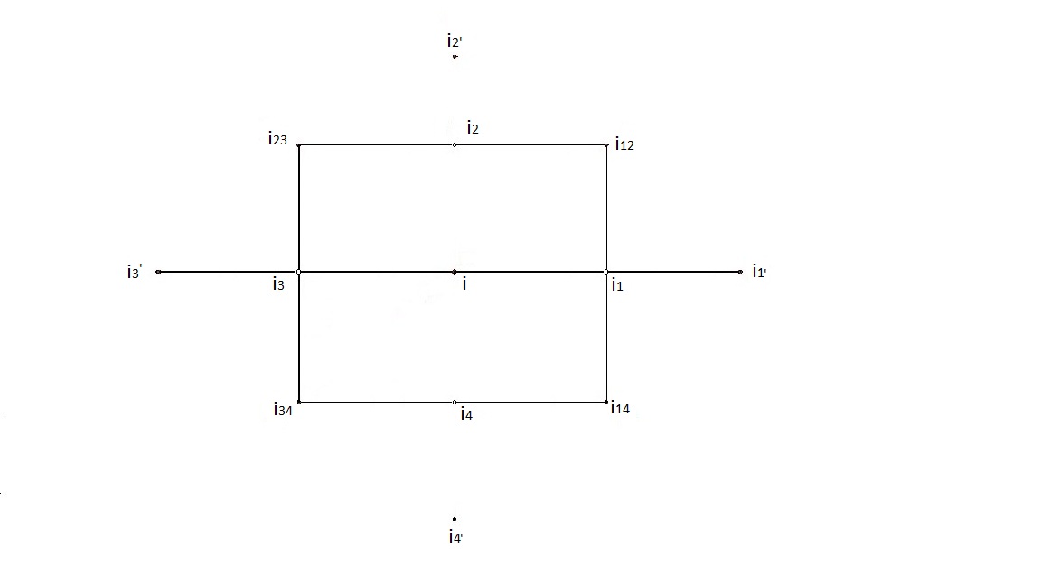
Figure 1. $\circ=\Gamma_{0}$, $\bullet=\Gamma_{1}$

If we denote $\{i_{1},i_{2},i_{3},i_{4}\}:=\{\sim i\}$ the neighbours of note $i$ as shown on Figure 1, and use Lemma 4.7 we get the following

$$\nu\|\nabla_{i}(\mathbb{E}^{\{\sim i\}}f)\|^{2}= \nu\|\nabla_{i}(\mathbb{E}^{i_{1}}\mathbb{E}^{\{i_{2},i_{3},i_{4}\}}f)\|^{2}\leq G_{1}\nu\|\nabla_{i}(\mathbb{E}^{\{i_{2},i_{3},i_{4}\}}f)\|^{2}+$$

(4.14) $$G_{1}\sum_{n=1}^{\infty}J^{n}\sum_{r:dist(r,i)=n}\ \nu(\|\nabla_{r}(\mathbb{E}^{\{i_{2},i_{3},i_{4}\}}f)\|^{2})$$

We will compute the second term in the right hand side of (4). For $n=1$ , we have

$$\sum_{dist(r,i)=1}\nu\|\nabla_{r}(\mathbb{E}^{\{i_{2},i_{3},i_{4}\}}f)\|^{2}= \nu\|\nabla_{i_{1}}(\mathbb{E}^{\{i_{2},i_{3},i_{4}\}}f)\|^{2}+\sum_{r=i_{2},i_{3},i_{4}}\nu\|\nabla_{r}(\mathbb{E}^{\{i_{2},i_{3},i_{4}\}}f)\|^{2}$$

(4.15) $$\leq \nu\|\nabla_{i_{1}}f\|^{2}$$

For $n=2$ , we distinguish between the nodes $r$ in $\{dist(r,i)=2\}$ which neighbour only one of the neighbours $\{i_{2},i_{3},i_{4}\}$ of $i$, which are the $i^{\prime}_{2},i^{\prime}_{3},i^{\prime}_{4},i_{12},i_{14}$, and these which neighbour two of the node in $\{i_{2},i_{3},i_{4}\}$, which are the $i_{23}$ and $i_{34}$ neighbouring $i_{2},i_{3}$ and $i_{3},i_{4}$ respectively, as shown in Figure 1. We can then write

$$\sum_{dist(r,i)=2}\nu\|\nabla_{r}(\mathbb{E}^{\{i_{2},i_{3},i_{4}\}}f)\|^{2} =\sum_{r=i_{23},i_{34}}\nu\|\nabla_{i}(\mathbb{E}^{\{i_{2},i_{3},i_{4}\}}f)\|^{2}+$$

(4.16) $$\sum_{r=i^{\prime}_{2},i^{\prime}_{3},i^{\prime}_{4},i_{12},i_{14}}\nu\|\nabla_{r}(\mathbb{E}^{\{i_{2},i_{3},i_{4}\}}f)\|^{2}$$

To bound the second term on the right hand side of (4), for any $r\in\{i^{\prime}_{2},i^{\prime}_{3},i^{\prime}_{4},i_{12},i_{14}\}$ neighbouring the node $t\in\{i_{2},i_{3},i_{4}\}$ we use Lemma 4.7

$$\nu\|\nabla_{r}(\mathbb{E}^{\{i_{2},i_{3},i_{4}\}}f)\|^{2}= \nu\|\nabla_{r}\mathbb{E}^{\{t\}}(\mathbb{E}^{\{i_{2},i_{3},i_{4}\}\smallsetminus\{t\}}f)\|^{2}\leq\nu\|\nabla_{r}(\mathbb{E}^{t}f)\|^{2}\leq$$

$$G_{1}\sum_{n=0}^{\infty}J^{n}\sum_{s:dist(s,r)=n}\ \nu(\|\nabla_{s}f\|^{2})$$

which leads to

$$\sum_{r=i^{\prime}_{2},i^{\prime}_{3},i^{\prime}_{4},i_{12},i_{14}}\nu\|\nabla_{r}(\mathbb{E}^{\{i_{2},i_{3},i_{4}\}}f)\|^{2}\leq G_{1}\sum_{dist(r,i)=2}\sum_{n=0}^{\infty}J^{n}\sum_{s:dist(s,r)=n}\ \nu(\|\nabla_{s}f\|^{2})$$

Since for nodes $r:dist(r,i)=2$, the nodes $s$ such that $dist(s,r)=n$ have distance from $i$ equal to $|n-2|$, $n$ or $n+2$ we get

$$\sum_{r=i^{\prime}_{2},i^{\prime}_{3},i^{\prime}_{4},i_{12},i_{14}}\nu \|\nabla_{r}(\mathbb{E}^{\{i_{2},i_{3},i_{4}\}}f)\|^{2}\leq 8G_{1}J\sum_{n=0}^{1}\sum_{r:dist(s,i)=n}\ \nu\|\nabla_{s}f\|^{2}+$$

(4.17) $$8G_{1}\sum_{n=2}^{\infty}J^{n-2}\sum_{r:dist(r,i)=n}\ \nu\|\nabla_{r}f\|^{2}$$

To bound the first term on the right hand side of (4), for example for $r=i_{23}$ neighbouring the nodes $i_{2}$ and $i_{3}$ we use again Lemma 4.7

(4.18) $$\nu\|\nabla_{i_{23}}(\mathbb{E}^{\{i_{2},i_{3},i_{4}\}}f)\|^{2}\leq\nu\|\nabla_{i_{23}}(\mathbb{E}^{\{i_{2},i_{3}\}}f)\|^{2}\leq G_{1}\sum_{n=0}^{\infty}J^{n}\sum_{s:dist(s,i_{23})=n}\ \nu\|\nabla_{s}(\mathbb{E}^{i_{3}}f)\|^{2}$$

The first term for $n=0$ on the sum of (4.18) by Lemma 4.7 is bounded by

$$\nu\|\nabla_{i_{23}}(\mathbb{E}^{i_{3}}f)\|^{2}\leq G_{1}\sum_{n=0}^{\infty}J^{n}\sum_{r:dist(s,i_{23})=n}\ \nu\|\nabla_{s}f\|^{2}\leq$$

$$\leq G_{1}J\sum_{n=0}^{1}\sum_{r:dist(s,i)=n}\ \nu\|\nabla_{s}f\|^{2}+$$

(4.19) $$G_{1}\sum_{n=2}^{\infty}J^{n-2}\sum_{r:dist(r,i)=n}\ \nu\|\nabla_{r}f\|^{2}$$

The terms for $n=1$ on the sum of (4.18) become

(4.20) $$G_{1}J\sum_{s:dist(s,i_{23})=1}\ \nu\|\nabla_{s}(\mathbb{E}^{i_{3}}f)\|^{2}\leq G_{1}J\sum_{s:dist(s,i)=1,3}\ \nu\|\nabla_{s}f\|^{2}$$

The terms for $n=2$ on the sum of (4.18) can be divided on those that neighbour $i_{3}$ and those that not

(4.21) $$\sum_{s:dist(s,i_{23})=2}\ \nu\|\nabla_{s}(\mathbb{E}^{i_{3}}f)\|^{2}= \sum_{s:dist(s,i_{23})=2,s\sim i_{3}}\ \nu\|\nabla_{s}(\mathbb{E}^{i_{3}}f)\|^{2}+\sum_{s:dist(s,i_{23})=2,s\nsim i_{3}}\ \nu\|\nabla_{s}(\mathbb{E}^{i_{3}}f)\|^{2}$$

For the second term on the right hand side of (4.21)

(4.22) $$\sum_{s:dist(s,i_{23})=2,s\nsim i_{3}}\ \nu\|\nabla_{s}(\mathbb{E}^{i_{3}}f)\|^{2}\leq\sum_{s:dist(s,i_{23})=2,s\nsim i_{3}}\ \nu\|\nabla_{s}f\|^{2}$$

While for the first term on the right hand side of (4.21) we can use Lemma 4.7

$$\sum_{s:dist(s,i_{23})=2,s\sim i_{3}}\ \nu\|\nabla_{s}(\mathbb{E}^{i_{3}}f)\|^{2}\leq G_{1}\sum_{s:dist(s,i_{23})=2,s\sim i_{3}}\sum_{n=0}^{\infty}J^{n}\sum_{r:dist(r,s)=n}\ \nu\|\nabla_{r}f\|^{2}\leq$$

$$\leq 4G_{1}\sum_{n=0}^{1}J^{n}\sum_{r:dist(s,i)=n}\ \nu\|\nabla_{s}f\|^{2}+$$

(4.23) $$4G_{1}\sum_{n=2}^{\infty}J^{n-2}\sum_{r:dist(r,i)=n}\ \nu\|\nabla_{r}f\|^{2}$$

From (4.21)-(4) we get the following bound for the terms for $n=2$ on the sum of (4.18)

$$G_{1}J^{2}\sum_{s:dist(s,i_{23})=2}\ \nu\|\nabla_{s}(\mathbb{E}^{i_{3}}f)\|^{2}\leq G_{1}J^{2}\sum_{s:dist(s,i)=2,4}\ \nu\|\nabla_{s}f\|^{2}+$$

(4.24) $$4G^{2}_{1}\sum_{n=0}^{\infty}J^{n}\sum_{r:dist(r,i)=n}\ \nu\|\nabla_{r}f\|^{2}$$

Finally, for the terms for $n>2$ on the sum on the right hand side of (4.18), we get

(4.25) $$G_{1}\sum_{n=3}^{\infty}J^{n}\sum_{r:dist(s,i_{23})=n}\ \nu\|\nabla_{s}(\mathbb{E}^{i_{3}}f)\|^{2}\leq G_{1}\sum_{n=3}^{\infty}J^{n-2}\sum_{r:dist(s,i)=n}\ \nu\|\nabla_{s}f\|^{2}$$

If we put (4), (4.20), (4) and (4.25) in (4.18) we get

$$\nu\|\nabla_{i_{23}}(\mathbb{E}^{\{i_{2},i_{3},i_{4}\}}f)\|^{2}\leq G_{2}\sum_{n=0}^{1}J^{n}\sum_{r:dist(s,i)=n}\ \nu\|\nabla_{s}f\|^{2}+$$

(4.26) $$G_{2}\sum_{n=2}^{\infty}J^{n-2}\sum_{r:dist(s,i)=n}\ \nu\|\nabla_{s}f\|^{2}$$

for $G_{2}=4G_{1}^{2}+3G_{1}$. Exactly the same bound can be obtain for the other term, $\nu\|\nabla_{i_{34}}(\mathbb{E}^{\{i_{2},i_{3},i_{4}\}}f)\|^{2}$, on the first sum of the right hand side of (4). Gathering together, (4), (4) and (4)

$$\sum_{dist(r,i)=2}\nu\|\nabla_{r}(\mathbb{E}^{\{i_{2},i_{3},i_{4}\}}f)\|^{2}= G_{3}\sum_{n=0}^{1}J^{n}\sum_{r:dist(s,i)=n}\ \nu\|\nabla_{s}f\|^{2}+$$

(4.27) $$G_{3}\sum_{n=2}^{\infty}J^{n-2}\sum_{r:dist(s,i)=n}\ \nu\|\nabla_{s}f\|^{2}$$

for $G_{3}=8G_{1}+2G_{2}$.

Furthermore, for every $r:dist(r,i)\geq 3$,

(4.28) $$\nu\|\nabla_{r}(\mathbb{E}^{\{i_{2},i_{3},i_{4}\}}f)\|^{2}\leq\nu\|\nabla_{r}f\|^{2}$$

Finally, if we put (4) and (4) and (4.28) in (4) we obtain

$$\nu\|\nabla_{i}(\mathbb{E}^{\{\sim i\}}f)\|^{2}= \nu\|\nabla_{i}(\mathbb{E}^{\{i_{1},i_{2},i_{3},i_{4}\}}f)\|^{2}\leq G_{1}\nu\|\nabla_{i}(\mathbb{E}^{\{i_{2},i_{3},i_{4}\}}f)\|^{2}+$$

(4.29) $$G_{4}\sum_{n=0}^{\infty}J^{n}\sum_{r:dist(r,i)=n}\ \nu\|\nabla_{r}f\|^{2}$$

for constant $G_{4}=G_{1}G_{3}+G_{1}$.

If we repeat the same calculation recursively for the first term on the right hand side of (4), then for $\nu\|\nabla_{i}(\mathbb{E}^{\{i_{3},i_{4}\}}f)\|^{2}$ and $\nu\|\nabla_{i}(\mathbb{E}^{\{i_{4}\}}f)\|^{2}$ we will finally obtain

$$\nu\|\nabla_{i}(\mathbb{E}^{\{\sim i\}}f)\|^{2}\leq G_{5}\sum_{n=0}^{\infty}J^{n}\sum_{r:dist(s,i)=n}\ \nu\|\nabla_{s}f\|^{2}$$

for a constant $G_{5}>1$. From the last inequality and (4.13) we get

$$\nu\|\nabla_{\Gamma_{1}}(\mathbb{E}^{\Gamma_{0}}f)\|^{2}\leq R_{1}\mathcal{\nu}\|\nabla_{\Gamma_{1}}f\|^{2}+R_{2}\nu\|\nabla_{\Gamma_{0}}f\|^{2}$$

for a constant $R_{2}\leq G_{5}J(\sum_{k=0}^{\infty}(4J)^{k})\leq\frac{JG_{5}}{1-4J}<1$ for $J$ sufficiently small such that $J<\min\{\frac{1}{4},\frac{1}{C_{5}+4}\}$. ∎

5. Second Sweeping out relations.

In this section we prove the second sweeping out relation. We start by first proving in the next lemma the second sweeping out relation between two neighbouring nodes.

Lemma 5.1.

Assume that the measure $\mu$ satisfies the log-Sobolev inequality and that the local specification has quadratic interactions $V$ as in (2). Then, for $J$ sufficiently small, for every $i\sim j$ the following sweeping out inequality holds

$$\nu\|\nabla_{i}(\mathbb{E}^{j}|f|^{2})^{\frac{1}{2}}\|^{2}\leq R_{3}\sum_{n=0}^{\infty}J^{n}\sum_{dist(r,i)=n}\ \nu\|\nabla_{r}f\|^{2}$$

for $R_{3}\geq 1$.

Proof.

Consider the (sub)gradient $\nabla_{i}=(X_{1}^{i},X_{2}^{i},...,X_{N}^{i})$. We can then write

(5.1) $$\|\nabla_{i}(\mathbb{E}^{j}f^{2})^{\frac{1}{2}}\|^{2}=\sum_{k=1}^{N}(X_{k}^{i}(\mathbb{E}^{j}f^{2})^{\frac{1}{2}})^{2}$$

Then for every $k\in\{1,...,N\}$ we can compute

(5.2) $$|X^{k}_{i}(\mathbb{E}^{j}f^{2})^{\frac{1}{2}}|^{2}= |\frac{1}{2}(\mathbb{E}^{j}f^{2})^{\frac{1}{2}-1}X^{k}_{i}(\mathbb{E}^{j}f^{2})|^{2}=\frac{1}{4}(\mathbb{E}^{j}f^{2})^{-1}|X^{k}_{i}(\mathbb{E}^{j}f^{2})|^{2}$$

But from relationship (4.2) of Lemma 4.1, if we put $f^{2}$ in $f$, we have

(5.3) $$|X^{k}_{i}(\mathbb{E}^{j}f^{2})|^{2}\leq 2|\int X^{k}_{i}(f^{2})\rho_{j}dx_{j}|^{2}+2|\int f^{2}(X^{k}_{i}\rho_{j})dx_{j}|^{2}$$

where again $\rho_{j}$ denotes the density of $\mathbb{E}^{j}$. For the second term in (5.3) we have

(5.4) $$|\int f^{2}(X^{k}_{i}\rho_{j})dx_{j}|^{2}\leq J^{2}|\mathbb{E}^{j}(f^{2};X^{k}_{i}V(x_{j},x_{i}))|^{2}$$

While for the first term of (5.3) the following bound holds

(5.5) $$|\int X^{k}_{i}(f^{2})\rho_{j}dx_{j}|^{2} =2|\mathbb{E}^{j}(f(X^{k}_{i}f))|^{2}\leq 2\left(\mathbb{E}^{j}f^{2}\right)\left(\mathbb{E}^{j}|X^{k}_{i}f|^{2}\right)$$

where above we used the Cauchy-Swartz ïnequality. If we plug (5.4) and (5.5) in (5.3) we get

(5.6) $$|X^{k}_{i}(\mathbb{E}^{j}f^{2})|^{2} \leq 4\left(\mathbb{E}^{j}f^{2}\right)\left(\mathbb{E}^{j}|X^{k}_{i}f|^{2}\right)+2J^{2}|\mathbb{E}^{j}(f^{2};X^{k}_{i}V(x_{j},x_{i})))|^{2}$$

Combining together (5.2) and (5.6) we obtain

(5.7) $$|X^{k}_{i}(\mathbb{E}^{j}f^{2})^{\frac{1}{2}}|^{2}\leq\mathbb{E}^{j}|X^{k}_{i}f|^{2}+J^{2}(\mathbb{E}^{j}f^{2})^{-1}|\mathbb{E}^{j}(f^{2};X^{k}_{i}V(x_{j},x_{i})))|^{2}$$

In order to calculate the second term on the right hand side of (5.7) we will use the following lemma.

Lemma 5.2.

For any probability measure $\mu$ the following inequality holds

$$\mu(|f|^{2};g)\leq\tilde{c}\left(\mu|f|^{2}\right)^{\frac{1}{2}}\left(\mu(|f-\mu f|^{2}(|g|^{2}+\mu|g|^{2}))\right)^{\frac{1}{2}}$$

for some constant $\tilde{c}$ uniformly on the boundary conditions.

Without loose of generality we can assume $\tilde{c}\geq 1$. The proof of Lemma 5.2 can be found in [Pa1]. Applying this bound to the second term in (5.7) leads to

$$\left(\mathbb{E}^{j}f^{2}\right)^{-1}|\mathbb{E}^{j}(f^{2};X^{k}_{i}V(x_{j},x_{i}))|^{2}\leq\tilde{c}^{2}\mathbb{E}^{j}\left[|f-\mathbb{E}^{j}f|^{2}\left((X^{k}_{i}V(x_{j},x_{i}))^{2}+\mathbb{E}^{j}(X^{k}_{i}V(x_{j},x_{i}))^{2}\right)\right]$$

From the last inequality and (5.7) we have

$$|X^{k}_{i}(\mathbb{E}^{j}f^{2})^{\frac{1}{2}}|^{2}\leq \mathbb{E}^{j}|X^{k}_{i}f|^{2}+J^{2}\tilde{c}^{2}\mathbb{E}^{j}\left[|f-\mathbb{E}^{j}f|^{2}(X^{k}_{i}V(x_{j},x_{i}))^{2}\right]+$$

$$J^{2}\tilde{c}^{2}\mathbb{E}^{j}\left[|f-\mathbb{E}^{j}f|^{2}\mathbb{E}^{j}(X^{k}_{i}V(x_{j},x_{i}))^{2}\right]$$

Putting this in (5.1) leads to

$$\|\nabla_{i}(\mathbb{E}^{j}f^{2})^{\frac{1}{2}}\|^{2}= \mathbb{E}^{j}\|\nabla_{i}f\|^{2}+J^{2}\tilde{c}^{2}\mathbb{E}^{j}\left[|f-\mathbb{E}^{j}f|^{2}\|\nabla_{i}V(x_{j},x_{i})\|^{2}\right]+$$

$$J^{2}\tilde{c}^{2}\mathbb{E}^{j}\left[|f-\mathbb{E}^{j}f|^{2}\mathbb{E}^{j}\|\nabla_{i}V(x_{j},x_{i})\|^{2}\right]$$

If we take the expectation with respect to the Gibbs measure and bound $\|\nabla_{i}V(x_{j},x_{i})\|^{2}$ by (2) we get

$$\nu\|\nabla_{i}(\mathbb{E}^{j}f^{2})^{\frac{1}{2}}\|^{2}\leq \nu\|\nabla_{i}f\|^{2}+2kJ^{2}\tilde{c}^{2}\nu\left[|f-\mathbb{E}^{j}f|^{2}d^{2}(x_{i})\right]+$$

$$kJ^{2}\tilde{c}^{2}\nu\left[|f-\mathbb{E}^{j}f|^{2}d^{2}(x_{j})\right]+kJ^{2}\tilde{c}^{2}\nu\left[|f-\mathbb{E}^{j}f|^{2}\mathbb{E}^{j}d^{2}(x_{j})\right]$$

If we bound the second and third term on the right hand side by Corollary 4.6 we get

$$\nu\|\nabla_{i}(\mathbb{E}^{j}f^{2})^{\frac{1}{2}}\|^{2}\leq \nu\|\nabla_{i}f\|^{2}+3kJ^{2}\tilde{c}^{2}D_{5}\nu(\|\nabla_{j}f\|^{2})+$$

$$3kJ^{2}\tilde{c}^{2}D_{5}\sum_{n=1}^{\infty}J^{n-1}\sum_{r:dist(r,j)=n}\ \nu(\|\nabla_{r}f\|^{2})+$$

(5.8) $$kJ^{2}\tilde{c}^{2}\nu\left[|f-\mathbb{E}^{j}f|^{2}\mathbb{E}^{j}d^{2}(x_{j})\right]$$

For the last term on the right hand side of (5) we can write

$$\nu\left[|f-\mathbb{E}^{j}f|^{2}\mathbb{E}^{j}d^{2}(x_{j})\right]=\nu\left[\mathbb{E}^{j}(|f-\mathbb{E}^{j}f|^{2})d^{2}(x_{j})\right]$$

and now apply the U-bound inequality (2.5) of Proposition 2.3

$$\nu\left[|f-\mathbb{E}^{j}f|^{2}\mathbb{E}^{j}d^{2}(x_{j})\right]\leq C\nu(\mathbb{E}^{j}(|f-\mathbb{E}^{j}f|^{2}))+$$

$$C\sum_{n=0}^{\infty}J^{n}\sum_{r:dist(r,j)=n}\ \nu\|\nabla_{r}(\mathbb{E}^{j}|f-\mathbb{E}^{j}f|^{2})^{\frac{1}{2}}\|^{2}$$

In order to bound the variance on the first term on the right hand side we can use the spectral gap type inequality of Lemma 4.5

$$\nu\left[|f-\mathbb{E}^{j}f|^{2}\mathbb{E}^{j}d^{2}(x_{j})\right]\leq CD_{4}\nu\|\nabla_{j}f\|^{2}+CD_{4}\sum_{n=1}^{\infty}J^{n-1}\sum_{r:dist(r,j)=n}\ \nu\|\nabla_{r}f^{2}\|+$$

(5.9) $$C\sum_{n=0}^{\infty}J^{n}\sum_{r:dist(r,j)=n}\ \nu\|\nabla_{r}(\mathbb{E}^{j}|f-\mathbb{E}^{j}f|^{2})^{\frac{1}{2}}\|^{2}$$

For $n=0$ the term of the second sum is zero, while for $n>1$ the nodes do not neighbour with $j$, so we have

$$\|\nabla_{r}(\mathbb{E}^{j}(|f-\mathbb{E}^{j}f|^{2}))^{\frac{1}{2}}\|^{2}= \sum_{k=1}^{N}|X_{k}^{r}(\mathbb{E}^{j}(|f-\mathbb{E}^{j}f|^{2}))^{\frac{1}{2}}|^{2}=$$

$$\frac{1}{4}\sum_{k=1}^{N}|(\mathbb{E}^{j}(|f-\mathbb{E}^{j}f|^{2}))^{-\frac{1}{2}}X^{r}_{k}(\mathbb{E}^{j}(|f-\mathbb{E}^{j}f|^{2})|^{2}\leq$$

$$\sum_{k=1}^{N}|(\mathbb{E}^{j}(|f-\mathbb{E}^{j}f|^{2}))^{-\frac{1}{2}}\mathbb{E}^{j}\left[(f-\mathbb{E}^{j}f)\left(|X^{r}_{k}f|+\mathbb{E}^{j}|X^{r}_{k}f|\right)\right]|^{2}$$

From Cauchy-Swartz inequality the last becomes

(5.10) $$\|\nabla_{r}(\mathbb{E}^{j}(|f-\mathbb{E}^{j}f|^{2}))^{\frac{1}{2}}\|^{2}\leq 2\sum_{k=1}^{N}\mathbb{E}^{j}|X^{r}_{k}f|^{2}=2\mathbb{E}^{j}\|\nabla_{r}f\|^{2}$$

Putting together (5) and (5.10)

$$\nu\left[|f-\mathbb{E}^{j}f|^{2}\mathbb{E}^{j}d^{2}(x_{j})\right]\leq CJ\sum_{r\sim j}\ \nu\|\nabla_{r}(\mathbb{E}^{j}|f-\mathbb{E}^{j}f|^{2})^{\frac{1}{2}}\|^{2}+CD_{4}\nu\|\nabla_{j}f\|^{2}+$$

(5.11) $$(CD_{4}+2C)\sum_{n=1}^{\infty}J^{n-1}\sum_{dist(r,j)=n}\ \nu\|\nabla_{r}f\|^{2}$$

From (5) and (5) we get

$$\nu\|\nabla_{i}(\mathbb{E}^{j}f^{2})^{\frac{1}{2}}\|^{2}\leq D_{6}\nu\|\nabla_{i}f\|^{2}+D_{6}J^{3}+D_{6}J\sum_{n=0}^{\infty}J^{n}\sum_{dist(r,j)=n}\ \nu\|\nabla_{r}f\|^{2}+$$

(5.12) $$\sum_{r\sim j}\ \nu\|\nabla_{r}(\mathbb{E}^{j}|f-\mathbb{E}^{j}f|^{2})^{\frac{1}{2}}\|^{2}$$

for a constant $D_{6}=1+k\tilde{c}^{2}(3D_{5}+CD_{4}+2C)$. If we replace $f$ by $f-\mathbb{E}^{j}f$ in (5) we get

$$\nu\|\nabla_{i}(\mathbb{E}^{j}(f-\mathbb{E}^{j}f)^{2})^{\frac{1}{2}}\|^{2}\leq D_{6}\nu\|\nabla_{i}(f-\mathbb{E}^{j}f)\|^{2}+D_{6}J^{3}\sum_{r\sim j}\ \nu\|\nabla_{r}(\mathbb{E}^{j}|f-\mathbb{E}^{j}f|^{2})^{\frac{1}{2}}\|^{2}+$$

$$D_{6}J\sum_{n=0}^{\infty}J^{n}\sum_{dist(r,j)=n}\ \nu\|\nabla_{r}(f-\mathbb{E}^{j}f)\|^{2}\leq$$

$$2D_{6}\nu\|\nabla_{i}f\|^{2}+2D_{6}\nu\|\nabla_{i}(\mathbb{E}^{j}f)\|^{2}+D_{6}J^{3}\sum_{r\sim j}\ \nu\|\nabla_{r}(\mathbb{E}^{j}|f-\mathbb{E}^{j}f|^{2})^{\frac{1}{2}}\|^{2}+$$

$$2D_{6}J^{2}\sum_{dist(r,j)=1}\ \nu\|\nabla_{r}(\mathbb{E}^{j}f)\|^{2}+2D_{6}J\sum_{n=0}^{\infty}J^{n}\sum_{dist(r,j)=n}\ \nu\|\nabla_{r}f\|^{2}$$

If we use Lemma 4.7 to bound the second and fourth term in the right hand side of the last inequality we obtain

$$\nu\|\nabla_{i}(\mathbb{E}^{j}(f-\mathbb{E}^{j}f)^{2})^{\frac{1}{2}}\|^{2}\leq 2D_{6}(G_{1}+1)\sum_{n=0}^{\infty}J^{n}\sum_{r:dist(r,i)=n}\ \nu\|\nabla_{r}f\|^{2}+$$

$$D_{6}J^{3}\sum_{r\sim j}\ \nu\|\nabla_{r}(\mathbb{E}^{j}|f-\mathbb{E}^{j}f|^{2})^{\frac{1}{2}}\|^{2}+$$

$$2G_{1}D_{6}J^{2}\sum_{dist(r,j)=1}\ \sum_{n=0}^{\infty}J^{n}\sum_{r:dist(s,r)=n}\ \nu\|\nabla_{s}f\|^{2}+$$

$$2D_{6}J\sum_{n=0}^{\infty}J^{n}\sum_{dist(r,j)=n}\ \nu\|\nabla_{r}f\|^{2}$$

Since $i$ and $j$ are neighbours and the $r$’s in the sum of the third term have distance less or equal to two from $i$, we can write

$$\nu\|\nabla_{i}(\mathbb{E}^{j}(f-\mathbb{E}^{j}f)^{2})^{\frac{1}{2}}\|^{2}\leq D_{7}\sum_{n=0}^{\infty}J^{n}\sum_{r:dist(r,i)=n}\ \nu\|\nabla_{r}f\|^{2}+$$

$$D_{7}J^{3}\sum_{r\sim j}\ \nu\|\nabla_{r}(\mathbb{E}^{j}|f-\mathbb{E}^{j}f|^{2})^{\frac{1}{2}}\|^{2}$$

for a constant $D_{7}=24D_{6}G_{1}+2D_{6}$. If we take the sum over all $i$ such that $i\sim j$ we get

$$\sum_{r\sim j}\nu\|\nabla_{r}(\mathbb{E}^{j}|f-\mathbb{E}^{j}f|^{2})^{\frac{1}{2}}\|^{2}\leq 4D_{7}\sum_{n=1}^{\infty}J^{n-1}\sum_{r:dist(r,j)=n}\ \nu\|\nabla_{r}f\|^{2}$$

$$4D_{7}J\nu\|\nabla_{j}f\|^{2}+$$

$$4D_{7}J^{3}\sum_{r\sim j}\ \nu\|\nabla_{r}(\mathbb{E}^{j}|f-\mathbb{E}^{j}f|^{2})^{\frac{1}{2}}\|^{2}$$

For $J$ sufficiently small so that $\frac{1}{1-4D_{6}J^{3}}<2$ we obtain

$$\sum_{r\sim j}\nu \|\nabla_{i}(\mathbb{E}^{j}|f-\mathbb{E}^{j}f|^{2})^{\frac{1}{2}}\|^{2}\leq 8D_{7}\sum_{n=1}^{\infty}J^{n-1}\sum_{r:dist(s,j)=n}\ \nu\|\nabla_{s}f\|^{2}+8D_{7}J\nu\|\nabla_{j}f\|^{2}$$

If we use the last inequality to bound the last term on the right hand side of (5) we obtain

$$\nu\|\nabla_{i}(\mathbb{E}^{j}f)^{\frac{1}{2}}\|^{2}\leq D_{6}\nu\|\nabla_{i}f\|^{2}+8D_{7}D_{6}J^{3}\sum_{n=1}^{\infty}J^{n-1}\sum_{r:dist(s,i)=n}\ \nu\|\nabla_{s}f\|^{2}+$$

$$D_{6}J\sum_{n=0}^{\infty}J^{n}\sum_{dist(r,j)=n}\ \nu\|\nabla_{r}f\|^{2}+8D_{6}D_{7}J^{4}\nu\|\nabla_{j}f\|^{2}$$

$$\leq 2D_{6}\nu\|\nabla_{i}f\|^{2}+(16D_{7}D_{6}J^{2}+D_{6})\sum_{n=1}^{\infty}J^{n}\sum_{r:dist(s,i)=n}\ \nu\|\nabla_{s}f\|^{2}$$

where above we used (4.9). This finishes the proof for an appropriate constant $R_{3}$. ∎

In the next proposition we will extend the sweeping out relations of the last lemma from the two neighboring nodes to the two infinite dimensional disjoint sets $\Gamma_{0}$ and $\Gamma_{1}$.

Proposition 5.3.

Assume that the measure $\mu$ satisfies the log-Sobolev inequality and that the local specification has quadratic interactions $V$ as in (2). Then, for $J$ sufficiently small, the following sweeping out inequality holds

(5.13) $$\nu\|\nabla_{\Gamma_{i}}(\mathbb{E}^{\Gamma_{j}}f^{2})^{\frac{1}{2}}\|^{2}\leq C_{1}\nu\|\nabla_{\Gamma_{i}}f\|^{2}+C_{2}\nu\|\nabla_{\Gamma_{j}}f\|^{2}$$

for $\{i,j\}=\{0,1\}$ and constants $C_{1}\in[1,\infty)$ and $0<C_{2}<1$.

Proof.

The proof will follow the same lines of the proof of Proposition 4.8. If we denote $\{\sim i\}=\{i_{1},i_{2},i_{3},i_{4}\}$ the neighbours of note $i$, then we can write

(5.14) $$\nu\|\nabla_{\Gamma_{1}}(\mathbb{E}^{\Gamma_{0}}f^{2})^{\frac{1}{2}}\|^{2}= \sum_{i\in\Gamma_{1}}\nu\|\nabla_{i}(\mathbb{E}^{\Gamma_{0}}f^{2})^{\frac{1}{2}}\|^{2}\leqslant\sum_{i\in\Gamma_{1}}\nu\|\nabla_{i}(\mathbb{E}^{\{\sim i\}}f^{2})^{\frac{1}{2}}\|^{2}$$

We can use Lemma 5.1 to bound the last one

$$\nu\|\nabla_{i}(\mathbb{E}^{\{\sim i\}}f^{2})^{\frac{1}{2}}\|^{2}= \nu\|\nabla_{i}(\mathbb{E}^{i_{1}}\mathbb{E}^{\{i_{2},i_{3},i_{4}\}}f^{2})^{\frac{1}{2}}\|^{2}\leq R_{3}\nu\|\nabla_{i}(\mathbb{E}^{\{i_{2},i_{3},i_{4}\}}f^{2})^{\frac{1}{2}}\|^{2}+$$

(5.15) $$R_{3}\sum_{n=1}^{\infty}J^{n}\sum_{dist(r,i)=n}\nu\|\nabla_{r}(\mathbb{E}^{\{i_{2},i_{3},i_{4}\}}f^{2})^{\frac{1}{2}}\|^{2}$$

We will compute the second term in the right hand side of (5). For $n=1$ , we have

$$\sum_{dist(r,i)=1}\nu\|\nabla_{r}(\mathbb{E}^{\{i_{2},i_{3},i_{4}\}}f^{2})^{\frac{1}{2}}\|^{2}= \nu\|\nabla_{i_{1}}(\mathbb{E}^{\{i_{2},i_{3},i_{4}\}}f^{2})^{\frac{1}{2}}\|^{2}+\sum_{r=i_{2},i_{3},i_{4}}\nu\|\nabla_{r}(\mathbb{E}^{\{i_{2},i_{3},i_{4}\}}f^{2})^{\frac{1}{2}}\|^{2}$$

(5.16) $$\leq \nu\|\nabla_{i_{1}}f\|^{2}$$

For $n=2$ , we distinguish between the nodes $r$ in $\{dist(r,i)=2\}$ which neighbour only one of the neighbours $\{i_{2},i_{3},i_{4}\}$ of $i$, which are the $i^{\prime}_{2},i^{\prime}_{3},i^{\prime}_{4},i_{12},i_{14}$, and these which neighbour two of the node in $\{i_{2},i_{3},i_{4}\}$, which are the $i_{23k}$ and $i_{34}$ neighbouring $i_{2},i_{3}$ and $i_{3},i_{4}$ respectively, as shown in Figure 1. We can then write

$$\sum_{dist(r,i)=2}\nu\|\nabla_{r}(\mathbb{E}^{\{i_{2},i_{3},i_{4}\}}f^{2})^{\frac{1}{2}}\|^{2} =\sum_{r=i_{23},i_{34}}\nu\|\nabla_{i}(\mathbb{E}^{\{i_{2},i_{3},i_{4}\}}f^{2})^{\frac{1}{2}}\|^{2}+$$

(5.17) $$\sum_{r=i^{\prime}_{2},i^{\prime}_{3},i^{\prime}_{4},i_{12},i_{14}}\nu\|\nabla_{r}(\mathbb{E}^{\{i_{2},i_{3},i_{4}\}}f^{2})^{\frac{1}{2}}\|^{2}$$

To bound the second term on the right hand side of (5), for any $r\in\{i^{\prime}_{2},i^{\prime}_{3},i^{\prime}_{4},i_{12},i_{14}\}$ neighbouring a node $t\in\{i_{2},i_{3},i_{4}\}$ we use Lemma 5.1

$$\nu\|\nabla_{r}(\mathbb{E}^{\{i_{2},i_{3},i_{4}\}}f^{2})^{\frac{1}{2}}\|^{2}= \nu\|\nabla_{r}\mathbb{E}^{\{t\}}(\mathbb{E}^{\{i_{2},i_{3},i_{4}\}\smallsetminus\{t\}}f^{2})^{\frac{1}{2}}\|^{2}\leq\nu\|\nabla_{r}(\mathbb{E}^{t}f^{2})^{\frac{1}{2}}\|^{2}\leq$$

$$R_{3}\sum_{n=0}^{\infty}J^{n}\sum_{r:dist(s,r)=n}\ \nu(\|\nabla_{s}f\|^{2})$$

which leads to

$$\sum_{r=i^{\prime}_{2},i^{\prime}_{3},i^{\prime}_{4},i_{12},i_{14}}\nu\|\nabla_{r}(\mathbb{E}^{\{i_{2},i_{3},i_{4}\}}f^{2})^{\frac{1}{2}}\|^{2}\leq\ R_{3}\sum_{dist(r,i)=2}\sum_{n=0}^{\infty}J^{n}\sum_{r:dist(s,r)=n}\ \nu\|\nabla_{s}f\|^{2}$$

Since for nodes $r:dist(r,i)=2$, the nodes $s$ such that $dist(s,r)=n$ have distance from $i$ equal to $n-2,n$ or $n+2$ we get

$$\sum_{r=i^{\prime}_{2},i^{\prime}_{3},i^{\prime}_{4},i_{12},i_{14}}\nu \|\nabla_{r}(\mathbb{E}^{\{i_{2},i_{3},i_{4}\}}f^{2})^{\frac{1}{2}}\|^{2}\leq 8R_{3}J^{2}\nu\|\nabla_{i}f\|^{2}+8R_{3}J\sum_{r:dist(s,i)=1}\ \nu\|\nabla_{s}f\|^{2}+$$

(5.18) $$8R_{3}\sum_{n=2}^{\infty}J^{n-2}\sum_{r:dist(s,i)=n}\ \nu\|\nabla_{s}f\|^{2}$$

To bound the first term on the right hand side of (5), for example for $r=i_{23}$ neighbouring the nodes $i_{2}$ and $i_{3}$ we use again Lemma 5.1

$$\nu\|\nabla_{i_{23}}(\mathbb{E}^{\{i_{2},i_{3},i_{4}\}}f^{2})^{\frac{1}{2}}\|^{2}\leq \nu\|\nabla_{i_{23}}(\mathbb{E}^{\{i_{2},i_{3}\}}f^{2})^{\frac{1}{2}}\|^{2}\leq$$

(5.19) $$R_{3}\nu\|\nabla_{i_{23}}(\mathbb{E}^{i_{3}}f^{2})^{\frac{1}{2}}\|^{2}+R_{3}\sum_{n=1}^{\infty}J^{n}\sum_{r:dist(s,i_{23})=n}\ \nu\|\nabla_{s}(\mathbb{E}^{i_{3}}f^{2})^{\frac{1}{2}}\|^{2}$$

The first term on the right hand side of (5) by Lemma 5.1 is bounded by

$$\nu\|\nabla_{i_{23}}(\mathbb{E}^{i_{3}}f^{2})^{\frac{1}{2}}\|^{2}\leq R_{3}\sum_{n=0}^{\infty}J^{n}\sum_{r:dist(s,i_{23})=n}\ \nu\|\nabla_{s}f\|^{2}\leq$$

$$\leq R_{3}J^{2}\nu\|\nabla_{i}f\|^{2}+R_{3}J\sum_{r:dist(s,i)=1}\ \nu\|\nabla_{s}f\|^{2}+$$

(5.20) $$R_{3}\sum_{n=2}^{\infty}J^{n-2}\sum_{r:dist(s,i)=n}\ \nu(\|\nabla_{s}f\|^{2})$$

The term for $n=1$ in the sum in the second term on the right hand side of (5) becomes

$$R_{3}J\sum_{r:dist(s,i_{23})=1}\ \nu\|\nabla_{s}(\mathbb{E}^{i_{3}}f^{2})^{\frac{1}{2}}\|^{2}\leq R_{3}J\sum_{r:dist(s,i_{23})=1}\ \nu\|\nabla_{s}f\|^{2}\leq$$

(5.21) $$\leq R_{3}J\sum_{r:dist(s,i)=1}\ \nu\|\nabla_{s}f\|^{2}+R_{3}J\sum_{r:dist(s,i)=3}\ \nu\|\nabla_{s}f\|^{2}$$

The terms for $n=2$ on the sum of (5) can be divided on those that neighbour $i_{23}$ and those that not

$$\sum_{s:dist(s,i_{23})=2}\ \nu\|\nabla_{s}(\mathbb{E}^{i_{3}}f^{2})^{\frac{1}{2}}\|^{2}= \sum_{s:dist(s,i_{23})=2,s\sim i_{3}}\ \nu\|\nabla_{s}(\mathbb{E}^{i_{3}}f^{2})^{\frac{1}{2}}\|^{2}+$$

(5.22) $$\sum_{s:dist(s,i_{23})=2,s\nsim i_{3}}\ \nu\|\nabla_{s}(\mathbb{E}^{i_{3}}f^{2})^{\frac{1}{2}}\|^{2}$$

For the second term on the right hand side of (5)

(5.23) $$\sum_{s:dist(s,i_{23})=2,s\nsim i_{3}}\ \nu\|\nabla_{s}(\mathbb{E}^{i_{3}}f^{2})^{\frac{1}{2}}\|^{2}\leq\sum_{s:dist(s,i_{23})=2,s\nsim i_{3}}\ \nu\|\nabla_{s}f\|^{2}$$

while for the first term on the right hand side of (5) we can use Lemma 5.1

$$\sum_{s:dist(s,i_{23})=2,s\sim i_{3}}\ \nu\|\nabla_{s}(\mathbb{E}^{i_{3}}f^{2})^{\frac{1}{2}}\|^{2}\leq R_{3}\sum_{s:dist(s,i_{23})=2,s\sim i_{3}}\sum_{n=0}^{\infty}J^{n}\sum_{r:dist(r,s)=n}\ \nu\|\nabla_{r}f\|^{2}\leq$$

$$\leq 4R_{3}\sum_{n=0}^{1}J^{n}\sum_{r:dist(s,i)=n}\ \nu\|\nabla_{s}f\|^{2}+$$

(5.24) $$4R_{3}\sum_{n=2}^{\infty}J^{n-2}\sum_{r:dist(r,i)=n}\ \nu\|\nabla_{r}f\|^{2}$$

From (5)-(5) we get the following bound for the terms for $n=2$ on the sum of (5)

$$R_{3}J^{2}\sum_{r:dist(s,i_{23})=2}\ \nu\|\nabla_{s}(\mathbb{E}^{i_{3}}f^{2})^{\frac{1}{2}}\|^{2}\leq R_{3}J^{2}\sum_{s:dist(s,i)=2,4}\ \nu\|\nabla_{s}f\|^{2}+$$

$$4R^{2}_{3}J^{2}\sum_{n=2}^{\infty}J^{n}\sum_{r:dist(r,i)=n}\ \nu\|\nabla_{r}f\|^{2}+$$

(5.25) $$4R^{2}_{3}\sum_{n=0}^{1}J^{n}\sum_{r:dist(r,i)=n}\ \nu\|\nabla_{r}f\|^{2}$$

For every $s:dist(s,i_{3})\geq 3$ we have $\nu\|\nabla_{s}(\mathbb{E}^{i_{3}}f^{2})^{\frac{1}{2}}\|^{2}\leq\nu\|\nabla_{s}f\|^{2}$, which gives

$$\sum_{n=3}^{\infty}J^{n}\sum_{r:dist(s,i_{23})=n}\ \nu\|\nabla_{s}(\mathbb{E}^{i_{3}}f^{2})^{\frac{1}{2}}\|^{2}\leq \sum_{n=3}^{\infty}J^{n}\sum_{r:dist(s,i_{23})=n}\ \nu\|\nabla_{s}f\|^{2}\leq$$

(5.26) $$\sum_{n=3}^{\infty}J^{n-2}\sum_{r:dist(s,i)=n}\ \nu\|\nabla_{s}f\|^{2}$$

since $dist(i_{23},i)=2$.

Putting (5), (5), (5) and (5) in (5) leads to

$$\nu\|\nabla_{i_{23}}(\mathbb{E}^{\{i_{2},i_{3},i_{4}\}}f^{2})^{\frac{1}{2}}\|^{2}\leq \nu\|\nabla_{i_{23}}(\mathbb{E}^{\{i_{2},i_{3}\}}f^{2})^{\frac{1}{2}}\|^{2}\leq$$

$$JR_{4}\nu\|\nabla_{i}f\|^{2}+JR_{4}\sum_{r:dist(s,i)=1}\ \nu\|\nabla_{s}f\|^{2}+$$

(5.27) $$R_{4}\sum_{n=2}^{\infty}J^{n-2}\sum_{r:dist(s,i)=n}\ \nu\|\nabla_{s}f\|^{2}$$

for $R_{4}=2R_{3}+5R^{2}_{3}$. The exact same bound can be obtain for the other term on the first sum of the right hand side of (5). Gathering together, (5), (5) and (5) leads to

$$\sum_{dist(r,i)=2}\nu\|\nabla_{r}(\mathbb{E}^{\{i_{2},i_{3},i_{4}\}}f^{2})^{\frac{1}{2}}\|^{2}\leq JR_{5}\nu\|\nabla_{i}f\|^{2}+JR_{5}\sum_{r:dist(s,i)=1}\ \nu\|\nabla_{s}f\|^{2}+$$

(5.28) $$R_{5}\sum_{n=2}^{\infty}J^{n-2}\sum_{r:dist(s,i)=n}\ \nu\|\nabla_{s}f\|^{2}$$

for $R_{5}=8R_{3}+R_{4}$.

Furthermore, for every $r:dist(r,i)\geq 3$,

(5.29) $$\nu\|\nabla_{r}(\mathbb{E}^{\{i_{2},i_{3},i_{4}\}}f^{2})^{\frac{1}{2}}\|^{2}\leq\nu\|\nabla_{r}f\|^{2}$$

Finally, if we put (5) and (5) and (5.29) in (5) we obtain

$$\nu\|\nabla_{i}(\mathbb{E}^{\{\sim i\}}f^{2})^{\frac{1}{2}}\|^{2}= \nu\|\nabla_{i}(\mathbb{E}^{\{i_{1},i_{2},i_{3},i_{4}\}}f^{2})^{\frac{1}{2}}\|^{2}\leq R_{3}\nu\|\nabla_{i}(\mathbb{E}^{\{i_{2},i_{3},i_{4}\}}f^{2})^{\frac{1}{2}}\|^{2}+$$

(5.30) $$+R_{6}\sum_{n=0}^{\infty}J^{n}\sum_{r:dist(s,i)=n}\ \nu\|\nabla_{s}f\|^{2}$$

for constant $R_{6}=R_{3}+R_{3}R_{5}$.

If we repeat the same calculation recursively, for the first term on the right hand side of (5), then for $\nu\|\nabla_{i}(\mathbb{E}^{\{i_{3},i_{4}\}}f^{2})^{\frac{1}{2}}\|^{2}$ and $\nu\|\nabla_{i}(\mathbb{E}^{\{i_{4}\}}f^{2})^{\frac{1}{2}}\|^{2}$ we will finally obtain

$$\nu\|\nabla_{i}(\mathbb{E}^{\{\sim i\}}f^{2})^{\frac{1}{2}}\|^{2}\leq R_{6}\sum_{n=3}^{\infty}J^{n}\sum_{r:dist(s,i)=n}\ \nu\|\nabla_{s}f\|^{2}$$

for a constant $R_{6}$. From the last inequality and (5.14) we get

$$\nu\|\nabla_{\Gamma_{1}}(\mathbb{E}^{\Gamma_{0}}f^{2})^{\frac{1}{2}}\|^{2}\leq C_{1}\nu\|\nabla_{\Gamma_{i}}f\|^{2}+C_{2}\nu\|\nabla_{\Gamma_{j}}f\|^{2}$$

for a constant $C_{2}\leq JR_{6}(\sum_{k=0}^{\infty}(4J)^{k})\leq\frac{JR_{6}}{1-4J}$ for $J$ sufficiently small such that $J<\frac{1}{4}$ and $J<\frac{1}{R_{6}-4}$ the proof of the proposition follows for $C_{2}<1$.

∎

6. log-Sobolev type inequalities.

Since the purpose of this paper is to prove the log-Sobolev inequality for the infinite dimensional Gibbs measure without assuming the log-Sobolev inequality for the one site measure $\mathbb{E}^{i,\omega}$, but the weaker inequality for the measure $\mu(dx_{i})=\frac{e^{\phi(x_{i})}dx_{i}}{\int\phi(x_{i})dx_{i}}$, we will show in this section that when the interactions are quadratic we can obtain a weaker log-Sobolev type inequality for the $\mathbb{E}^{i,\omega}$ measure. This will be the object of the next proposition.

Proposition 6.1.

Assume that the measure $\mu$ satisfies the log-Sobolev inequality and that the local specification has quadratic interactions $V$ as in (2). Then, for $J$ sufficiently small, the one site measure $\mathbb{E}^{i,\omega}$ satisfies the following log-Sobolev type inequality

$$\nu\mathbb{E}^{i,\omega}\left(f^{2}\log\frac{f^{2}}{\mathbb{E}^{i,\omega}f^{2}}\right)\leq c_{1}\nu\|\nabla_{i}f\|^{2}+c_{1}\sum_{n=1}^{\infty}J^{n-1}\sum_{r:dist(r,i)=n}\ \nu(\|\nabla_{r}f\|^{2})$$

for some positive constant $c_{1}$.

Proof.

Assume $g\geq 0$. We start with our main assumption that the measure $\mu(dx)=\frac{e^{\phi(x)}dx}{\int\phi(x)dx}$ satisfies the log-Sobolev inequality for a constant $c_{0}$, that is

(6.1) $$\mu(g^{2}\log\frac{g^{2}}{\mu g^{2}})\leq c_{0}\mu\|\nabla_{i}g\|^{2}$$

We will interpolate this inequality to create the entropy with respect to the one site measure $\mathbb{E}^{i,\omega}$ in the left hand side. For this we will first define the function

$$V^{i}=\sum_{j\sim i}J_{i,j}V(x_{i},\omega_{j})$$

Notice that $V^{i}\geq 0$. Then inequality (6.1) for $g=e^{\frac{-V^{i}}{2}}f,f\geq 0$ gives

$$\int e^{-\phi(x_{i})} (e^{-V^{i}}f^{2}\log\frac{e^{-V^{i}}f^{2}}{\int e^{-\phi(x_{i})}(e^{-V^{i}}f^{2})dx_{i}/\int e^{-\phi(x_{i})}dx_{i}})dx_{i}$$

(6.2) $$\ \ \ \ \ \ \ \ \ \ \ \ \ \ \ \ \ \ \ \ \ \ \ \ \ \ \ \ \ \ \ \ \ \ \leq c_{0}\int e^{-\phi(x_{i})}\|\nabla_{i}(e^{\frac{-V^{i}}{2}}f)\|^{2}dx_{i}$$

Denote by $S_{r}$ and $S_{l}$ the right and left hand side of (6.2) respectively. If we use the Leibnitz rule for the gradient on the right hand side of (6.2) we have

$$S_{r}\leq 2c_{0}\int e^{-\phi(x_{i})}\|e^{\frac{{-V^{i}}}{2}}(\nabla_{i}f)\|^{2}dx_{i}+2c_{0}\int e^{-\phi(x_{i})}\|f(\nabla_{i}e^{\frac{{-V^{i}}}{2}})\|^{2}dx_{i}=$$

(6.3) $$\left(\int e^{-\phi(x_{i})-V^{i}}f^{2}dx_{i}\right)c_{0}2\left(\mathbb{E}^{i,\omega}\|\nabla_{i}f\|^{2}+\frac{1}{4}\mathbb{E}^{i,\omega}f^{2}\|\nabla_{i}{V^{i}}\|^{2}\right)$$

On the left hand side of (6.2) we form the entropy for the measure $\mathbb{E}^{i,\omega}$ measure with Hamiltonian $\phi(x_{i})+V^{i}$.

$$S_{l}= \int e^{-\phi(x_{i})-V^{i}}f^{2}log\frac{f^{2}}{\int e^{-\phi(x_{i})-V^{i}}f^{2}dx_{i}/\int e^{-\phi(x_{i})-V^{i}}dx_{i}}dx_{i}$$

$$+\int e^{-\phi(x_{i})-V^{i}}f^{2}\log\frac{\left(\int e^{-\phi(x_{i})}dx_{i}\right)e^{-V^{i}}}{\int e^{-\phi(x_{i})-V^{i}}dx_{i}}dx_{i}$$

$$= (\int e^{-\phi(x_{i})-V^{i}}f^{2}dx_{i})\left(\mathbb{E}^{i,\omega}(f^{2}log\frac{f^{2}}{\mathbb{E}^{i,\omega}f^{2}})-\mathbb{E}^{i,\omega}(f^{2}V^{i})\right)$$

$$+\int e^{-\phi(x_{i})-V^{i}}f^{2}log\frac{\int e^{-\phi(x_{i})}dx_{i}}{\int e^{-\phi(x_{i})-V^{i}}dx_{i}}dx_{i}$$

Since $V^{i}$ is no negative, the last equality leads to

(6.4) $$S_{l}\geq(\int e^{-\phi(x_{i})-V^{i}}f^{2}dx_{i})\left(\mathbb{E}^{i,\omega}(f^{2}log\frac{f^{2}}{\mathbb{E}^{i,\omega}f^{2}})-\mathbb{E}^{i,\omega}(f^{2}V^{i})\right)$$

If we combine (6.2) together with (6) and (6.4) we obtain

$$\mathbb{E}^{i,\omega}(f^{2}log\frac{f^{2}}{\mathbb{E}^{i,\omega}f^{2}})\leq 2c_{0}\mathbb{E}^{i,\omega}\|\nabla_{i}f\|^{2}+\mathbb{E}^{i,\omega}(f^{2}(\frac{c_{0}\|\nabla_{i}V^{i}\|^{2}}{2}+V^{i}))$$

If take the expectation with respect to the Gibbs measure in the last relationship we have

(6.5) $$\nu(f^{2}log\frac{f^{2}}{\mathbb{E}^{i,\omega}f^{2}})\leq 2c_{0}\nu\|\nabla_{i}f\|^{2}+\nu(f^{2}(\frac{c_{0}\|\nabla_{i}V^{i}\|^{2}}{2}+V^{i}))$$

From [B-Z] and [R] the following estimate of the entropy holds

(6.6) $$\mathbb{E}^{i,\omega}(f^{2}log\frac{f^{2}}{\mathbb{E}^{i,\omega}f^{2}})\leq A\mathbb{E}^{i,\omega}(f-\mathbb{E}^{i,\omega}f)^{2}+\mathbb{E}^{i,\omega}(f-\mathbb{E}^{i,\omega}f)^{2}log\frac{(f-\mathbb{E}^{i,\omega}f)^{2}}{\mathbb{E}^{i,\omega}(f-\mathbb{E}^{i,\omega}f)^{2}}$$

for some positive constant $A$. If we take expectations with respect to the Gibbs measure at the last inequality we get

(6.7) $$\nu(|f|^{2}log\frac{|f|^{2}}{\mathbb{E}^{i,\omega}|f|^{2}})\leq A\nu|f-\mathbb{E}^{i,\omega}f|^{2}+\nu(|f-\mathbb{E}^{i,\omega}f|^{2}log\frac{|f-\mathbb{E}^{i,\omega}f|^{2}}{\mathbb{E}^{i,\omega}|f-\mathbb{E}^{i,\omega}f|^{2}})$$

We can now use (6.5) to bound the second term on the right hand side of (6.7). Then we will obtain

$$\nu(f^{2} log\frac{f^{2}}{\mathbb{E}^{i,\omega}f^{2}})\leq A\nu|f-\mathbb{E}^{i,\omega}f|^{2}+2c_{0}\nu\|\nabla_{i}f\|^{2}+\nu(|f-\mathbb{E}^{i,\omega}f|^{2}(\frac{c_{0}\|\nabla_{i}{V^{i}}\|^{2}}{2}+V^{i}))\leq$$

$$A\nu|f-\mathbb{E}^{i,\omega}f|^{2}+2c_{0}\nu\|\nabla_{i}f\|^{2}+\sum_{j\sim i}J_{i,j}\nu(|f-\mathbb{E}^{i,\omega}f|^{2}(2c_{0}\|\nabla_{i}{V(x_{i},\omega_{j})}\|^{2}+V(x_{i},\omega_{j})))$$

If we take under account that we are considering quadratic interactions and bound $V$ and $\|\nabla_{i}{V^{i}}\|^{2}$ by (2) we get

$$\nu(f^{2} log\frac{f^{2}}{\mathbb{E}^{i,\omega}f^{2}})\leq(A+4)\nu|f-\mathbb{E}^{i,\omega}f|^{2}+2c_{0}\nu\|\nabla_{i}f\|^{2}+$$

$$4(2c_{0}+1)kJ\nu(|f-\mathbb{E}^{i,\omega}f|^{2}d^{2}(x_{i}))+(2c_{0}+1)kJ\sum_{j\sim i}\nu(|f-\mathbb{E}^{i,\omega}f|^{2}d^{2}(\omega_{j}))$$

where above we also used that $V(x_{i},\omega_{j})\leq 1+\left|V(x_{i},\omega_{j})\right|^{2}$. We can bound the first term on the right hand side by Lemma 4.5 and the third and the fourth term by Corollary 4.6.

$$\nu(f^{2}log\frac{f^{2}}{\mathbb{E}^{i,\omega}f^{2}})\leq c_{1}\nu\|\nabla_{i}f\|^{2}+c_{1}\sum_{n=1}^{\infty}J^{n-1}\sum_{r:dist(r,i)=n}\ \nu(\|\nabla_{r}f\|^{2})$$

which finishes the proof of the proposition for $c_{1}=(A+4)4(D_{L}+D_{3})+6(2c_{0}+1)kD_{5}$.∎

We now prove a log-Sobolev type inequality for the product measure $\mathbb{E}^{\Gamma_{k}}$ for $k=0,1$.

Proposition 6.2.

Assume that the measure $\mu$ satisfies the log-Sobolev inequality and that the local specification has quadratic interactions $V$ as in (2). Then, for $J$ sufficiently small, the following log-Sobolev type inequality for the product measures $\mathbb{E}^{\Gamma_{k},\omega}$ holds

$$\nu\mathbb{E}^{\Gamma_{k}}(f^{2}log\frac{f^{2}}{\mathbb{E}^{\Gamma_{k}}f^{2}})\leq\tilde{C}\nu\|\nabla_{\Gamma_{0}}f\|^{2}+\tilde{C}\nu\|\nabla_{\Gamma_{1}}f\|^{2}$$

for $k=0,1$, and some positive constant $\tilde{C}$.

Proof.

We will prove Proposition 6.2 for $k=1$, that is

$$\nu\mathbb{E}^{\Gamma_{1}}(f^{2}log\frac{f^{2}}{\mathbb{E}^{\Gamma_{1}}f^{2}})\leq\tilde{C}\nu\|\nabla_{\Gamma_{0}}f\|^{2}+\tilde{C}\nu\|\nabla_{\Gamma_{1}}f\|^{2}$$

for $f\geq 0$.

In the proof of this proposition we will use the following estimation. For any $i\in\mathbb{Z}$ and $\{\sim i\}=i_{1},i_{2},i_{3},i_{4}$ denote

$$\Theta(i): =\nu\|\nabla_{i}(\mathbb{E}^{\{i_{1},i_{2},i_{3},i_{4}\}}f^{2})^{\frac{1}{2}}\|^{2}+\nu\|\nabla_{i}(\mathbb{E}^{\{i_{2},i_{3},i_{4}\}}f^{2})^{\frac{1}{2}}\|^{2}+$$

$$+\nu\|\nabla_{i}(\mathbb{E}^{\{i_{3},i_{4}\}}f^{2})^{\frac{1}{2}}\|^{2}+\nu\|\nabla_{i}(\mathbb{E}^{\{i_{4}\}}f^{2})^{\frac{1}{2}}\|^{2}$$

and

$$\Lambda(i):=\sum_{n=0}^{\infty}J^{n}\sum_{r:dist(s,i)=n}\ \nu\|\nabla_{s}f\|^{2}$$

From the calculations of the components of the sum of $\Theta(i)$ in the proof of Proposition 5.3 and the recursive inequality (5) we can surmise that there exists an $R_{7}>0$ such that

(6.8) $$\Theta(i)\leq R_{7}\Lambda(i)$$

We start with the following enumeration of the nodes in $\Gamma_{1}$ as depicted in figure 2.

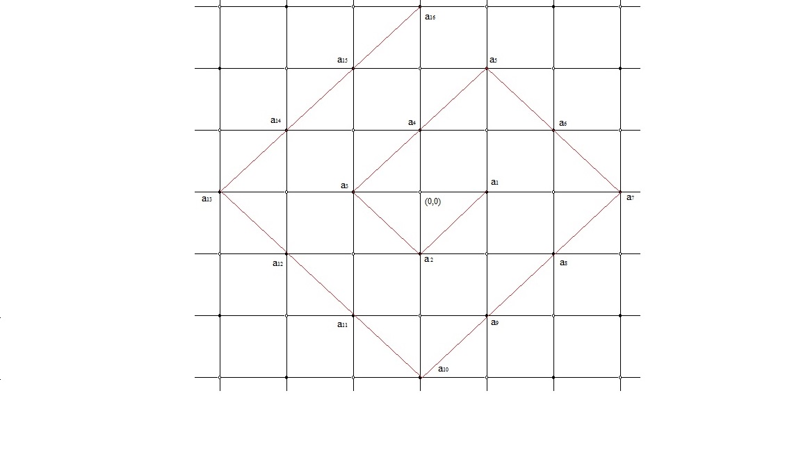
Figure 2. $\circ=\Gamma_{0}$, $\bullet=\Gamma_{1}$

Denote the nodes in $\Gamma_{1}$ closest to $(0,0)$, that is the neighbours of $(0,0)$ and name them $a_{1},a_{2},a_{3},a_{4}$, with $a_{1}$ being any of the four and the rest named clockwise. Then choose any of the nodes in $\Gamma_{1}$ of distance two from $a_{4}$ and distance three from $(0,0)$, and name it $a_{5}$ and continue clockwise the enumeration with the rest of the nodes in $\Gamma_{1}$ of distance three form $(0,0)$. Then the same for the nodes of $\Gamma_{1}$ of distance four from $(0,0)$. We continue with the same way with the nodes in $\Gamma_{1}$ of higher distances from $(0,0)$, moving clockwise while we move away from $(0,0)$. In this way the nodes in $\Gamma_{1}$ are enumerated in a spiral way moving clockwise away from $(0,0)$. In that way we can write $\mathbb{E}^{\Gamma_{1}}=\sqcap_{i=1}^{+\infty}\ \mathbb{E}^{a_{i}}$.

Then the entropy of the product measure $\mathbb{E}^{\Gamma_{1}}$ can be calculated by being expressed in terms of the entropies of single nodes in $\Gamma_{1}$ for which we have shown a log-Sobolev type inequality in Proposition 6.1.

(6.9) $$\nu\mathbb{E}^{\Gamma_{1}}(f^{2}\log\frac{f^{2}}{\mathbb{E}^{\Gamma_{1}}f^{2}})=\sum_{k=1}^{+\infty}\nu\mathbb{E}^{a_{k}}(\mathbb{E}^{a_{k-1}}...\mathbb{E}^{a_{1}}f^{2}\log\frac{\mathbb{E}^{a_{k-1}}...\mathbb{E}^{a_{1}}f^{2}}{\mathbb{E}^{a_{k}}...\mathbb{E}^{a_{1}}f^{2}})$$

To compute the entropies in the right hand side of (6.9) we will use the log-Sobolev type inequality for the one site measure $\mathbb{E}^{k}$ from Proposition 6.1.

(6.10) $$\nu\mathbb{E}^{a_{k}}(\mathbb{E}^{a_{k-1}}...\mathbb{E}^{a_{1}}f^{2}\log\frac{\mathbb{E}^{a_{k-1}}...\mathbb{E}^{a_{1}}f^{2}}{\mathbb{E}^{a_{k}}...\mathbb{E}^{a_{1}}f^{2}})\leq c_{1}\nu\|\nabla_{a_{k}}f\|^{2}+$$

$$c_{1}\sum_{n=1}^{\infty}J^{n-1}\sum_{j:dist(j,a_{k})=n}\ \nu\|\nabla_{j}(\mathbb{E}^{a_{k-1}}...\mathbb{E}^{a_{1}}f^{2})^{\frac{1}{2}}\|^{2}$$

where above we used that $\nu\|\nabla_{a_{k}}(\mathbb{E}^{a_{k-1}}...\mathbb{E}^{a_{1}}f^{2})^{\frac{1}{2}}\|^{2}\leq\nu\|\nabla_{a_{k}}f\|^{2}$, since by the way the spiral was constructed it’s elements do not neighbour with each other. For every $j$ that neighbours with at least one of the $a_{k-1},a_{k-2},...,a_{1}$ we have that

$$\nu\|\nabla_{j}(\mathbb{E}^{a_{k-1}}...\mathbb{E}^{a_{1}}f^{2})^{\frac{1}{2}}\|^{2}\leq\Theta(j)$$

which because of (6.8) implies

(6.11) $$\nu\|\nabla_{j}(\mathbb{E}^{a_{k-1}}...\mathbb{E}^{a_{1}}f^{2})^{\frac{1}{2}}\|^{2}\leq R_{7}\Lambda(j)$$

For every $j$ that does not neighbour with any of the $a_{k-1},a_{k-2},...,a_{1}$ we have that

(6.12) $$\nu\|\nabla_{j}(\mathbb{E}^{a_{k-1}}...\mathbb{E}^{a_{1}}f^{2})^{\frac{1}{2}}\|^{2}\leq\nu\|\nabla_{j}f\|^{2}$$

Putting (6.11) and (6.12) in (6.10) we obtain

$$\nu\mathbb{E}^{a_{k}}(\mathbb{E}^{a_{k-1}}...\mathbb{E}^{a_{1}}f^{2}\log\frac{\mathbb{E}^{a_{k-1}}...\mathbb{E}^{a_{1}}f^{2}}{\mathbb{E}^{a_{k}}...\mathbb{E}^{a_{1}}f^{2}})\leq c_{1}\nu\|\nabla_{a_{k}}f\|^{2}+$$

$$c_{1}R_{7}\sum_{n=1}^{\infty}J^{n-1}\sum_{j:dist(j,a_{k})=n}\Lambda(j)+$$

$$c_{1}\sum_{n=1}^{\infty}J^{n-1}\sum_{j:dist(j,a_{k})=n}\nu\|\nabla_{j}f\|^{2}$$

Combining this with (6.9)

$$\nu\mathbb{E}^{\Gamma_{1}}(f^{2}\log\frac{f^{2}}{\mathbb{E}^{\Gamma_{1}}f^{2}})\leq c_{1}\sum_{k=1}^{+\infty}\nu\|\nabla_{a_{k}}f\|^{2}+$$

$$c_{1}R_{7}\sum_{k=1}^{+\infty}\sum_{n=1}^{\infty}J^{n-1}\sum_{j:dist(j,a_{k})=n}\Lambda(j)+$$

$$c_{1}R_{7}\sum_{k=1}^{+\infty}\sum_{n=1}^{\infty}J^{n-1}\sum_{j:dist(j,a_{k})=n}\nu\|\nabla_{j}f\|^{2}$$

Since in the last two sums above, for every $j\in\mathbb{Z}^{2}$, the terms $\Lambda(j)$ and $\nu\|\nabla_{j}f\|^{2}$ appear one time for every $i\in\Gamma_{1}$ with a coefficient $J^{dist({i,j)-1}}$, the accompanying coefficient for any of these terms is $\frac{\sum_{k=0}^{\infty}(4J)^{k}}{J}$ since for every node $j$, $\#\{i:dist(i,j)=n\}\leq 4^{n}$. So by rearranging the terms in the last inequality we get

$$\nu\mathbb{E}^{\Gamma_{1}}(f^{2}\log\frac{f^{2}}{\mathbb{E}^{\Gamma_{1}}f^{2}})\leq c_{1}\nu\|\nabla_{\Gamma_{1}}f\|^{2}+\frac{R_{7}c_{1}}{J}\sum_{j\in\mathbb{Z}^{2}}\left(\sum_{n=0}^{\infty}(4J)^{n}\right)\Lambda(j)+$$

$$\frac{R_{7}c_{1}}{J}\sum_{j\in\mathbb{Z}^{2}}\sum_{n=0}^{\infty}(4J)^{n}\nu\|\nabla_{j}f\|^{2}$$

$$= c_{1}\nu\|\nabla_{\Gamma_{1}}f\|^{2}+\frac{R_{7}c_{1}}{J(1-4J)}\sum_{j\in\mathbb{Z}^{2}}\Lambda(j)+\frac{R_{7}c_{1}}{J(1-4J)}\sum_{j\in\mathbb{Z}^{2}}\nu\|\nabla_{j}f\|^{2}$$

for $J<\frac{1}{4}$. For the first sum

$$\sum_{j\in\mathbb{Z}^{2}}\Lambda(j) =\sum_{j\in\mathbb{Z}^{2}}\sum_{n=0}^{\infty}J^{n}\sum_{r:dist(s,j)=n}\ \nu\|\nabla_{s}f\|^{2}\leq\sum_{j\in\mathbb{Z}^{2}}\left(\sum_{n=0}^{\infty}(4J)^{n}\right)\nu\|\nabla_{j}f\|^{2}$$

$$=\frac{1}{1-4J}\sum_{j\in\mathbb{Z}^{2}}\nu\|\nabla_{j}f\|^{2}$$

We finally get

$$\nu\mathbb{E}^{\Gamma_{1}}(f^{2}\log\frac{f^{2}}{\mathbb{E}^{\Gamma_{1}}f^{2}})\leq c_{1}\nu\|\nabla_{\Gamma_{1}}f\|^{2}+\frac{2R_{7}c_{1}}{J(1-4J)^{2}}\sum_{j\in\mathbb{Z}^{2}}\nu\|\nabla_{j}f\|^{2}$$

∎

7. spectral gap and proof of main theorem

In Proposition 6.1 and Proposition 6.2 we showed a log-Sobolev type inequality for the one site measure $\mathbb{E}^{i,\omega}$and then obtained a similar inequality through it for the product measures $\mathbb{E}^{\Gamma_{i},\omega},i=0,1$. In Lemma 4.5 a spectral gap type inequality was also shown for the one site measure $\mathbb{E}^{i,\omega}$ for both cases. In the following proposition the spectral gap type inequality of Lemma 4.5 will be extended to the product measure $\mathbb{E}^{\Gamma_{i},\omega},i=0,1$. However, this does not happen through the Spectral Gap type inequality for the one site measure $\mathbb{E}^{i,\omega}$ of Lemma 4.5 but through the log-Sobolev type inequality for $\mathbb{E}^{\Gamma_{i},\omega},i=0,1$ of Proposition 6.2.

Proposition 7.1.

Assume that the measure $\mu$ satisfies the log-Sobolev inequality and that the local specification has quadratic interactions $V$ as in (2). Then, for $J$ sufficiently small, the following spectral gap type inequality holds

$$\nu|f-\mathbb{E}^{\Gamma_{i},\omega}f|^{2}\ \leq\tilde{R}\nu\|\nabla_{\Gamma_{0}}f\|^{2}+\tilde{R}\nu\|\nabla_{\Gamma_{1}}f\|^{2}$$

for $i=0,1$ and some positive constant $\tilde{R}$.

The proof of this proposition is based in the use of the log-Sobolev type inequality for the product measures $\mathbb{E}^{\Gamma_{k}},k=0,1$ of Proposition 6.2 and the sweeping out relations for the same measures from Proposition 4.8. The proof of this proposition is presented in Lemma 7.1 of [Pa1].

Spectral Gap inequalities have been associated with convergence to equilibrium and ergodic properties. In the next proposition we will use the weaker spectral gap inequality for the product measures $\mathbb{E}^{\Gamma_{i},\omega},i=0,1$ of Proposition 7.1 to show the a.e. convergence of $\mathcal{P}^{n}$ to the infinite dimensional Gibbs measure $\nu$, where $\mathcal{P}^{n}$ is defined as follows

(7.1) $$\mathcal{P}^{n}f=\begin{cases}f&n=0\\ \mathbb{E}^{\Gamma_{0}}\mathcal{P}^{n-1}f&n\text{\ odd}\\ \mathbb{E}^{\Gamma_{1}}\mathcal{P}^{n-1}f&n\text{\ even\ }>0\end{cases}$$

Proposition 7.2.

Assume that the measure $\mu$ satisfies the log-Sobolev inequality and that the local specification has quadratic interactions $V$ as in (2). Then, for $J$ sufficiently small, and $\mathcal{P}$ as in (7.1), $\mathcal{P}^{n}f$ converges $\nu$-a.e. to the Gibbs measure $\nu$.

Proof.

We will follow closely [G-Z]. We will compute the variance of the $\mathcal{P}^{n}f$ with respect to the product measure $\mathbb{E}^{\Gamma_{k}}$ for $k=0$ or $1$ when $n$ is odd or even respectively. For this we will use the spectral gap type inequality for the product measures $\mathbb{E}^{\Gamma_{i},\omega},i=0,1$ presented in Proposition 7.1.

$$\nu|\mathcal{P}^{n}f-\mathcal{P}^{n+1}f|^{2}= \nu|\mathcal{P}^{n}f-\mathbb{E}^{\Gamma_{k}}\mathcal{P}^{n}f|^{2}\leq\tilde{R}\nu\|\nabla_{\Gamma_{0}}\mathcal{P}^{n}f\|^{2}+\tilde{R}\nu\|\nabla_{\Gamma_{1}}\mathcal{P}^{n}f\|^{2}=$$

$$= \tilde{R}\nu\|\nabla_{\Gamma_{k}}\mathcal{P}^{n}f\|^{2}=\tilde{R}\nu\|\nabla_{\Gamma_{k}}\mathbb{E}^{\Gamma_{1-k}}\mathcal{P}^{n-1}f\|^{2}$$

where $k$ above is $0$ or $1$ if $n$ is odd or even respectively. If we use the first sweeping out inequality of Proposition 4.8 we get

$$\nu|\mathcal{P}^{n}f-\mathcal{P}^{n+1}f|^{2}\leq \tilde{R}R_{1}\nu\|\nabla_{\Gamma_{k}}\mathcal{P}^{n-1}f\|^{2}+\tilde{R}R_{2}\nu\|\nabla_{\Gamma_{1-k}}\mathcal{P}^{n-1}f\|^{2}=\tilde{R}R_{2}\nu\|\nabla_{\Gamma_{1-k}}\mathcal{P}^{n-1}f\|^{2}$$

where we recall $R_{2}\leq\frac{JG_{6}}{1-4J}<1$. If we apply $n-2$ more times Proposition 4.8 we obtain the following bound

(7.2) $$\nu|\mathcal{P}^{n}f-\mathcal{P}^{n+1}f|^{2}\leq\tilde{R}R_{2}^{n-2}\left(R_{1}\nu\|\nabla_{\Gamma_{1}}f\|^{2}+R_{2}\nu\|\nabla_{\Gamma_{0}}f\|^{2}\right)$$

which converges to zero as $n$ goes to infinity, because $R_{2}<1$. If we define the sets

$$\Delta_{n}=\{|\mathcal{P}^{n}f-\mathcal{P}^{n+1}f|\geq\frac{1}{2^{n}}\}$$

we can calculate

$$\nu(\Delta_{n})=\nu\left(\left\{|\mathcal{P}^{n}f-\mathcal{P}^{n+1}f|\geq\frac{1}{2^{n}}\right\}\right)\leq 2^{2n}\nu|\mathcal{P}^{n}f-\mathcal{P}^{n+1}f|^{2}$$

by Chebyshev inequality. If we use (7.2) to bound the last one we get

$$\nu(\Delta_{n})\leq(4R_{2})^{n-2}8\tilde{R}\left(R_{1}\nu\|\nabla_{\Gamma_{1}}f\|^{2}+R_{2}\nu\|\nabla_{\Gamma_{0}}f\|^{2}\right)$$

and for $J$ sufficiently small such that $4R_{2}\leq\frac{4JG_{6}}{1-4J}<\frac{1}{2}$ (recall that $R_{2}\leq\frac{JG_{6}}{1-4J}$) we have that

$$\sum_{n=0}^{\infty}\nu(\Delta_{n})\leq\left(\sum_{n=0}^{\infty}\frac{1}{2^{n}}\right)64\tilde{R}\left(R_{1}\nu\|\nabla_{\Gamma_{1}}f\|^{2}+R_{2}\nu\|\nabla_{\Gamma_{0}}f\|^{2}\right)<\infty$$

Thus,

$$\{\mathcal{P}^{n}f-\nu\mathcal{P}^{n}f\}_{n\in\mathbb{N}}$$

converges $\nu-$almost surely by the Borel-Cantelli lemma. Furthermore,

$$\mathcal{P}^{n}f\rightarrow\vartheta\ (f)\ \ \ \ \ \nu-\text{a.e.}$$

We will first show that $\theta(f)$ is a constant, which means that it does not depend on variables on $\Gamma_{0}$ or $\Gamma_{1}$. We first notice that $\mathcal{P}^{n}(f)$ is a function on $\Gamma_{0}$ or $\Gamma_{1}$ when $n$ is odd or even respectively. This implies that the limits

$$\vartheta_{o}(f):=\lim_{n\text{\ odd},n\rightarrow\infty}\mathcal{P}^{n}f\text{ \ and \ }\vartheta_{e}(f):=\lim_{n\text{\ even},n\rightarrow\infty}\mathcal{P}^{n}f$$

do not depend on variables on $\Gamma_{0}$ and $\Gamma_{1}$ respectively. However, since the two subsequences $\{\mathcal{P}^{n}f\}_{n\text{\ even}}$ and $\{\mathcal{P}^{n}f\}_{n\text{\ odd}}$ converge to $\vartheta(f)$ $\nu-$a.e. we conclude that

$$\vartheta_{o}(f)=\vartheta(f)=\vartheta_{e}(f)$$

which implies that $\theta(f)$ is a constant. From that we obtain that

(7.3) $$\nu\left(\vartheta(f)\right)=\vartheta(f)$$

Since the sequence $\{\mathcal{P}^{n}f\}_{n\in\mathbb{N}}$ converges $\nu-$almost, the same holds for the sequence $\{\mathcal{P}^{n}f-\nu\mathcal{P}^{n}f\}_{n\in\mathbb{N}}$.

It remains to show that $\vartheta(f)=\nu(f)$. At first we show this for positive bounded functions $f$. In this case we have

(7.4) $$\lim_{n\rightarrow\infty}(\mathcal{P}^{n}f-\nu\mathcal{P}^{n}f)=\vartheta(f)-\nu\left(\vartheta(f)\right)=\vartheta(f)-\vartheta(f)=0$$

by the dominated convergence theorem and (7.3). On the other hand, we also have

(7.5) $$\lim_{n\rightarrow\infty}(\mathcal{P}^{n}f-\nu\mathcal{P}^{n}f)=\lim_{n\rightarrow\infty}(\mathcal{P}^{n}f-\nu f)=\vartheta(f)-\nu(f)$$

where above we used the definition of the Gibbs measure $\nu$. From (7.4) and (7.5) we get that

$$\vartheta(f)=\nu(f)$$

for bounded functions $f$. We now extend it to no bounded positive functions $f$. Consider $f_{k}(x):=\max\{f(x),k\}$ for any $k\in\mathbb{N}$. Then

$$\vartheta(f_{k})=\lim_{n\rightarrow\infty}\mathcal{P}^{n}f_{k}=\nu f_{k},\ \ \nu\ \ a.e.$$

since $f_{k}(x)$ is bounded by $k$. Then since $f_{k}$ is increasing on $k$, by the monotone convergence theorem we obtain

$$\vartheta(f)=\lim_{k\rightarrow\infty}\vartheta(f_{k})=\lim_{k\rightarrow\infty}\nu(f_{k})=\nu(\lim_{k\rightarrow\infty}f_{k})=\nu(f)\ \ \nu\ \ a.e.$$

The assertions then can be extended to no positive functions $f$ by writing $f=f^{+}-f^{-}$, where $f^{+}=\max\{f,0\}$ and $f^{-}=-\min\{f,0\}$. ∎

We can now proceed with the proof of the main theorem.

7.1. proof Proposition 2.3

The proof of the main result will be based on the iterative method developed by Zegarlinski in [Z1] and [Z2] (see also [Pa1] and [I-P] for similar application). We will start with a lemma that shows the iterative step.

Denote $Ent_{\mu}(f):=\mu(f^{2}\log\frac{f^{2}}{\mu f^{2}})$ the entropy of a function $f$ with respect to a measure $\mu$.

Lemma 7.3.

Assume $\mathcal{P}$ as in (7.1). For any $n\geq 1$,

(7.6) $$\mathcal{P}^{n}[f\log f]= \sum_{m=0}^{n-1}\mathcal{P}^{n-m-1}[Ent_{\mathbb{E}^{\Gamma_{k}}}(\mathcal{P}^{m}f)]+\mathcal{P}^{n}f\log\mathcal{P}^{n}f$$

where $k$ above is $0$ or $1$ if $n$ is odd or even respectively.

Proof.

One observes that for any $\Lambda\subset\mathbb{Z}^{2}$

(7.7) $$Ent_{\mathbb{E}^{\Lambda}}(g)=\mathbb{E}^{\Lambda}\left(g\log\frac{g}{\mathbb{E}^{\Lambda}g}\right)=\mathbb{E}^{\Lambda}[g\log g]-\\ (\mathbb{E}^{\Lambda}g)\log(\mathbb{E}^{\Lambda}g)$$

The statement (7.6) for $n=1$ can be trivially derived from (7.7) if we put $\Lambda=\Gamma_{0}$ and $g=f$. Assuming (7.6) is true for some $n\geq 0$, we prove it for $n+1$. Apply (7.7) with $\Lambda=\Gamma_{k}$ and $\mathcal{P}^{n}f$ in the place of $g$, where $k$ above is $0$ or $1$ if $n$ is odd or even respectively:

$$\mathbb{E}^{\Gamma_{k}}[(\mathcal{P}^{n}f)\log(\mathcal{P}^{n}f)] =Ent_{\mathbb{E}^{\Gamma_{k}}}(\mathcal{P}^{n}f)+(\mathbb{E}^{\Gamma_{k}}\mathcal{P}^{n}f)\log(\mathbb{E}^{\Gamma_{k}}\mathcal{P}^{n}f)$$

$$=Ent_{\mathbb{E}^{\Gamma_{k}}}(\mathcal{P}^{n}f)+(\mathcal{P}^{n+1}f)\log(\mathcal{P}^{n+1}f)$$

Using this, and applying $\mathbb{E}^{\Gamma_{k}}$ to (7.6) we obtain (7.6) for $n+1$. ∎

Using Proposition 7.2 we have $\mathcal{P}^{n}[f\log f]\to\nu[f\log f]$ and $\mathcal{(P}^{n}f)\log(\mathcal{(P}^{n}f)\to\nu[f]\log\nu[f]$, $\nu$-a.e. From this and Fatou’s lemma, (7.6) gives

$$Ent_{\nu}(f^{2}) \leq\liminf_{n\to\infty}\bigg{\{}\nu\bigg{[}\sum_{m=0}^{n-1}\mathcal{P}^{n-m-1}[Ent_{\mathbb{E}^{\Gamma_{k}}}(\mathcal{P}^{m}f)]\bigg{]}\bigg{\}}$$

(7.8) $$=\liminf_{n\to\infty}\bigg{\{}\sum_{m=0}^{n-1}\nu[Ent_{\mathbb{E}^{\Gamma_{k}}}(\mathcal{P}^{m}f^{2})]\bigg{\}}$$

where we used the fact that $\nu$ is a Gibbs measure to obtain the last equality. If we use Proposition 6.2 to bound the first term of the first sum we have

$$\nu Ent_{\mathbb{E}^{\Gamma_{0}}}(f^{2})\leq\tilde{C}\nu\|\nabla_{\Gamma_{0}}f\|^{2}+\tilde{C}\nu\|\nabla_{\Gamma_{1}}f\|^{2}$$

Similarly, for $m\geq 1$, we can use Proposition 6.2 and then we get

$$\nu[Ent_{\mathbb{E}^{\Gamma_{k}}}(\mathcal{P}^{m}f^{2})] \leq\tilde{C}\nu\|\nabla_{\Gamma_{k}}\sqrt{\mathcal{P}^{m}f^{2}}\|^{2}\leq\tilde{C}[C_{1}C_{2}^{m-1}\nu\|\nabla_{\Gamma_{1}}f\|^{2}+C_{2}^{m}\nu\|\nabla_{\Gamma_{0}}f\|^{2}]$$

where, for the last inequalities we used Proposition 5.3 and induction. Substituting in (7.8), we obtain (recall that $0<C_{2}<1$)

$$Ent_{\nu}(f^{2})\leq\frac{\tilde{C}C_{1}}{C_{2}(1-C_{2})}\nu\|\nabla_{\Gamma_{1}}f\|^{2}+\frac{\tilde{C}}{1-C_{2}}\nu\|\nabla_{\Gamma_{0}}f\|^{2}\leq\overline{C}\,\nu\|\nabla f\|^{2}$$

where $\overline{C}$ is the largest of the two coefficients. This ends the proof of the log-Sobolev inequality for $\nu$.

∎

References

- [A-S] S. Aida and D.W. Stroock , Moment Estimates Derived From Poincaré and Logarithmic Sobolev Inequalities, Math. Res. Lett., 1, 75-86 (1994).
- [A-B-C] C. Ané, S. Blachère, D. Chafaï, P. Fougères, I. Gentil, F. Malrieu, C. Roberto and G. Scheffer, Sur les inégalités de Sobolev logarithmiques, Panoramas et Synthèses. Soc. Math, 10, France, Paris (2000).
- [B] D. Bakry, L’hypercontractivitè et son utilisation en théorie des semigroups, Séminaire de Probabilités XIX, Lecture Notes in Math., 1581, Springer, New York, 1-144 (1994).
- [B-E] D. Bakry and M. Emery, Difusions hypercontractives ,Seminaire de Probabilites XIX, Springer Lecture Notes in Math. 1123, 177-206 (1985).
- [B-HK] J. Bellisard and R. Hoegn-Krohn, Compactness and the maximal Gibbs state for random fields on the Lattice, Commun. Math. Phys., 84, 297-327 (1982).
- [B-G] S.G. Bobkov and F. Gotze, Exponential integrability and transportation cost related to logarithmic sobolev inequalities , J of Funct Analysis 163 1-28 (1999).
- [B-L] S.G. Bobkov and M. Ledoux, From Brunn-Minkowski to Brascamp-Lieb and to Logarithmic Sobolev Inequalities, Geom. funct. anal. 10, 1028-1052 (2000).
- [B-L-U] A. Bonfiglioni, E. Lanconelli and F. Uguzzoni, Stratified Lie groups and Potential Theory for their Sub-Laplacians, Springer Monographs in Mathematics. Springer, New York (2007).
- [B-Z] S.G. Bobkov and B. Zegarlinski, Entropy Bounds and Isoperimetry. Memoirs of the American Mathematical Society, Vol: 176, 1 - 69 (2005).
- [B-H] T. Bodineau and B. Helffer, Log-Sobolev inequality for unbounded spin systems , J of Funct Analysis 166, 168-178 (1999).
- [D-S] J.D. Deuschel and D. Stroock, Large Deviations , Academic Press, San Diego (1989).
- [D] R. L. Dobrushin, The problem of uniqueness of a Gibbs random field and the problem of phase transition, Funct. Anal. Apll. 2, 302-312 (1968).
- [G-R] I. Gentil and C. Roberto, Spectral Gaps for Spin Systems: Some Non-convex Phase Examples, J. Func. Anal., 180, 66-84 (2001).
- [G] L. Gross, Logarithmic Sobolev inequalities, Am. J. Math. 97, 1061-1083 (1976).
- [G-Z] A.Guionnet and B.Zegarlinski, Lectures on Logarithmic Sobolev Inequalities, IHP Course 98, pp 1-134 in Seminare de Probabilite XXVI, Lecture Notes in Mathematics 1801, Springer (2003).
- [H-Z] W.Hebisch and B.Zegarlinski, Coercive inequalities on metric measure spaces. J. Func. Anal., 258, 814-851 (2010).
- [H] B. Helffer, Semiclassical Analysis, Witten Laplacians and Statistical Mechanics, Partial Differential Equations and Applications. World Scientific, Singapore (2002).
- [I-K-P] J. Inglis, T. Konstantopoulos and I. Papageorgiou, Log-Sobolev inequalities for Infinite Dimensional Gibbs measures with non-quadratic interactions. (preprint)
- [I-P] J. Inglis and I. Papageorgiou, Logarithmic Sobolev Inequalities for Infinite Dimensional Hörmander Type Generators on the Heisenberg Group. Potential Anal., 31, 79-102 (2009).
- [M1] K. Marton, An inequality for relative entropy and logarithmic Sobolev inequalities in Eucledian spaces. J. Func. Anal., 264, 34-61 (2013).
- [M2] K. Marton, Logarithmic Sobolev inequalities in discreet product spaces: A proof by a transportation cost distance. (Arxiv: 1507.02803).
- [O-R] F. Otto and M. Reznikoff, A new criterion for the Logarithmic Sobolev Inequality and two Applications , J. Func. Anal., 243, 121-157 (2007).
- [Pa1] I. Papageorgiou, The Logarithmic Sobolev Inequality in Infinite dimensions for Unbounded Spin Systems on the Lattice with non Quadratic Interactions, Markov Proc. Related Fields, 16, 447-484 (2010).
- [Pa2] I. Papageorgiou, A note on the Modified Log-Sobolev inequality . Potential Anal., 35, 275-286 (2011).
- [Pa3] I. Papageorgiou, The logarithmic Sobolev inequality for Gibbs measures on infinite product of Heisenberg groups. Markov Proc. Related Fields, 20, 705-749 (2014).
- [Pr] C.J.Preston,Random Fields, LNM 534, Springer (1976).
- [R-Z] C. Roberto and B. Zegarlinski, Orlicz-Sobolev inequalities for sub-Gaussian measures and ergodicity of Markov semi-groups , J. Func. Anal., 243 (1), 28-66 (2007).
- [R] O. Rothaus, Analytic inequalities, isoperimetric inequalities and logarithmic Sobolev inequalities, J. Func. Anal., 64, 296-313 (1985).
- [SC] L.Saloff-Coste, Aspects of Sobolev-Type Inequalities, London Mathematical Society Lecture Note Series, 289. Cambridge University Press, Cambridge, (2002).
- [S-Z] D.W. Stroock and B. Zegarlinski, The equivalence of the Logarithmic Sobolev Inequalities and the Dobrushin Shlosman Mixing condition, Comm. Math. Phys. 144, 303-323 (1992).
- [V-SC-C] N. Th. Varopoulos, L. Saloff-Coste and T. Coulhon, Analysis and Geometry on Groups, Tracts in Mathematics, 100, Cambridge University Press, Cambridge, (1992).
- [Y] N.Yoshida, The log-Sobolev inequality for weakly coupled lattice field, Probab.Theor. Relat. Fields 115, 1-40 (1999).
- [Z1] B. Zegarlinski, On log-Sobolev Inequalities for Infinite Lattice Systems, Lett. Math. Phys. 20, 173-182 (1990).
- [Z2] B. Zegarlinski, The strong decay to equilibrium for the stochastic dynamics of unbounded spin systems on a lattice, Comm. Math. Phys. 175, 401-432 (1996).