Conductance in inhomogeneous quantum wires:
Luttinger liquid predictions and quantum Monte Carlo results

Abstract

We study electron and spin transport in interacting quantum wires contacted by noninteracting leads. We theoretically model the wire and junctions as an inhomogeneous chain where the parameters at the junction change on the scale of the lattice spacing. We study such systems analytically in the appropriate limits based on Luttinger liquid theory and compare the results to quantum Monte Carlo calculations of the conductances and local densities near the junction. We first consider an inhomogeneous spinless fermion model with a nearest-neighbor interaction and then generalize our results to a spinful model with an onsite Hubbard interaction.

I Introduction

An important tool to study the physics of quantum wires is measurements of their conductance as a function of parameters such as the filling fraction or temperature.Liang et al. (2001); Javey et al. (2003); Yacoby et al. (1996); Steinberg et al. (2008); Tarucha et al. (1995); Purewal et al. (2007); KamataKumada et al. (2014) In order to understand the results of such experiments it is important to find an appropriate model not only for the quantum wire itself but for the full system including the leads. Typically, the properties of the quantum wire are strongly affected by electron-electron interactions. Fermi liquid theory has to be replaced by Luttinger liquid theory in one dimension.Tomonaga (1950); Luttinger (1963); Giamarchi (2004) The leads, on the other hand, form a higher-dimensional electron gas in which interactions can be neglected. This suggests that a lead-wire-lead system can be modeled as an inhomogeneous quantum wire where the interaction and hopping parameters, as well as the chemical potential, change at the junctions. A sketch of such a setup and how it is modeled as an inhomogeneous wire is shown in Fig. 1. Quantum wires have been analyzed using Luttinger liquid theory previously and it has been shown that for perfect adiabatic contacts the conductance of the wire is controlled by the parameters of the lead rather than of the wireYue et al. (1994); Safi and Schulz (1995); Maslov and Stone (1995); Ogata and Fukuyama (1994); Wong and Affleck (1994); de Chamon and Fradkin (1997); Safi and Schulz (1999); Imura et al. (2002); Enss et al. (2005); *Janzen2006; Rech and Matveev (2008a, b); Gutman et al. (2010); Thomale and Seidel (2011); Sedlmayr et al. (2012, 2013, 2014). The conductance for adiabatic contacts with noninteracting leads is therefore given by the perfect quantum conductance, $G=ne^{2}/h$ for $n$ channels, instead of being renormalized by the Luttinger liquid of the wire as might be expected from a naive calculation for an infinite wire. However, for any reasonably sharp junction there will be scattering at the junction even for otherwise perfect ballistic connections. Such scattering becomes renormalized by the interaction and can lead to a vanishing d.c. conductance in the low temperature limit for repulsive interactions.Kane and Fisher (1992a, b); Eggert and Affleck (1992); Furusaki and Nagaosa (1993, 1996); Pereira and Miranda (2004); Sedlmayr et al. (2011)

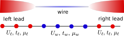
Figure 1: (Color online) A quantum wire connected to two noninteracting leads. The identical leads are modeled as a chain with hopping $t_{\ell}$, chemical potential $\mu_{\ell}$, and interaction $U_{\ell}=0$. The wire has parameters $U_{w},\,t_{w},\,\mu_{w}$. The junction between the leads and the wire is modeled as being abrupt.

In two recent papersSedlmayr et al. (2012, 2014) we have shown that for an inhomogeneous spinless fermion model as depicted in Fig. 1 it is, however, still possible to obtain perfect conductance by tuning the parameters of the wire and the leads. Using Luttinger liquid calculations and a comparison with numerical quantum Monte Carlo (QMC) results for static local response functions it was possible to establish the existence of a highly nontrivial conducting fixed point described by two effective Luttinger liquid parameters.Sedlmayr et al. (2012, 2014) Here, we want to generalize these studies in two ways. First, we will check the existence of conducting fixed points more directly by calculating the conductance numerically using QMC. Second, we will generalize the study of the conductance in inhomogeneous wires to spinful systems. We will concentrate on two microscopic models: (1) The spinless fermionic chain with Hamiltonian $H=H_{0}+H_{I}$ where

$$H_{0} = -\sum_{j}\left(t_{j}\Psi_{j+1}^{\dagger}\Psi_{j}+\textrm{H.c.}+\mu_{j}n_{j}\right)\,,\textrm{ and}$$

$$H_{I} = \sum_{j}U_{j}n_{j}n_{j+1}\,.$$ (1)

Here $\Psi_{j}^{(\dagger)}$ is the annihilation (creation) operator of a spinless fermion at site $j$ and $n_{j}=\Psi_{j}^{\dagger}\Psi_{j}$ is the density operator. The site-dependent parameters $t_{j},\mu_{j}$ and $U_{j}$ are defined as shown in Fig. 1. (2) The inhomogeneous Hubbard model:

$$H_{0} = -\sum_{j,\sigma}\big{(}t_{j}\Psi_{j+1,\sigma}^{\dagger}\Psi_{j,\sigma}+\textrm{H.c.}+\mu_{j}n_{j}\big{)}\,,\textrm{ and}$$

$$H_{I} = \sum_{j}U_{j}n_{j,\uparrow}n_{j,\downarrow}\,,$$ (2)

where $\Psi_{j,\sigma}^{(\dagger)}$ is now the annihilation (creation) operator of an electron with spin $\sigma$. The particle number for each spin species is given by $n_{j,\sigma}=\Psi_{j,\sigma}^{\dagger}\Psi_{j,\sigma}$ and the total number operator is $n_{j}=n_{j,\uparrow}+n_{j,\downarrow}$. For the numerical simulations we will consider systems with periodic boundary conditions with half of the system representing the noninteracting leads and the other half the interacting quantum wire. It is important to note that the backscattering at the two junctions will not influence each other as long as we ensure that the distance between the junctions is large compared to the correlation length in the quantum wire, $\xi\sim u/T$, where $u$ is the velocity of elementary excitations and $T$ the temperature.

Our paper is organized as follows. In Sec. II we will introduce the QMC method used to calculate the conductance and discuss cases of homogeneous and inhomogeneous wires where exact results are available which can be used to check the accuracy of the numerical results. In Sec. III we then present results for the spinless fermionic chain, Eq. (I). Next, we derive the bosonized theory for the inhomogeneous Hubbard chain in Sec. IV and compare the theoretical predictions with QMC data. We summarize our main results and discuss some of the remaining open questions in Sec. V.

II QMC method

We have implemented a quantum Monte Carlo (QMC) algorithm, the stochastic series expansion (SSE),Sandvik (1992) to calculate imaginary time correlation functions.Dorneich and Troyer (2001) The conductance of the wire in linear response can then be obtained from these imaginary time correlation functions.Louis and Gros (2003) We calculate the linear response to an infinitesimal drop in electric and magnetic field at site $k$ for charge and spin respectively

$$P_{k}^{c} = e\sum\limits_{m>k}(n_{m,\uparrow}+n_{m,\downarrow})$$ (3)

$$P_{k}^{s} = \frac{\mu_{\text{B}}}{2}\sum\limits_{m>k}(n_{m,\uparrow}-n_{m,\downarrow})\,,$$

where $e$ is the elementary charge, $m$ is the site, and $\mu_{\text{B}}$ the Bohr magneton. Accordingly, we define a local charge and spin current operator

$$j_{k}^{c} = \mathrm{i}t_{k}e\sum\limits_{\sigma}({\psi}^{\dagger}_{k,\sigma}{\psi}_{k+1,\sigma}-{\psi}^{\dagger}_{k+1,\sigma}{\psi}_{k,\sigma})$$

$$j_{k}^{s} = \frac{\mathrm{i}t_{k}\mu_{\text{B}}}{2}\left[({\psi}^{\dagger}_{k,\uparrow}{\psi}_{k+1,\uparrow}-{\psi}^{\dagger}_{k+1,\uparrow}{\psi}_{k,\uparrow})\right.$$

$$\hskip 28.45274pt-\left.({\psi}^{\dagger}_{k,\downarrow}{\psi}_{k+1,\downarrow}-{\psi}^{\dagger}_{k+1,\downarrow}{\psi}_{k,\downarrow})\right]\,.$$

Following Ref. Louis and Gros, 2003 we calculate the charge and spin conductance ($\nu=c,s$) in linear response using

$$g^{\nu}_{x,y}(\omega_{n}) = -\frac{\omega_{n}}{\hbar}\,\mbox{Re}\,\int\limits_{0}^{\hbar\beta}\textrm{e}^{\mathrm{i}\omega_{n}\tau}\langle P^{\nu}_{x}P^{\nu}_{y}(\mathrm{i}\tau)\rangle\,\mathrm{d}\tau\,,$$ (5)

$$= -\frac{\omega_{n}}{\hbar}\int\limits_{0}^{\hbar\beta}\cos(\omega_{n}\tau)\langle P^{\nu}_{x}P^{\nu}_{y}(\mathrm{i}\tau)\rangle\,\mathrm{d}\tau$$

where $y=0$ is the location of the perturbation $P_{y}$ (quadratic in the Fermi operators) and $x$ is the location where we determine the response to that perturbation, where $|x-y|$ must be small. Here $\omega_{n}=2\pi n/\beta$ are the bosonic Matsubara frequencies, which are used to extrapolate to $\omega=0$ to obtain the d.c. conductance. For the spinless fermionic chain (I) we can only define a charge conductance using a voltage drop $P_{k}^{c}=e\sum_{m>k}n_{m}$. The charge current operator $j_{k}^{c}$ is then defined as in Eq. (II) but without the spin index $\sigma$.

Numerically, the task of obtaining conductances is now reduced to calculating expectation values in imaginary time. The technique for this is described in Ref. Dorneich and Troyer, 2001. QMC provides us with the expectation values $\langle P^{\nu}_{x}P^{\nu}_{y}(\mathrm{i}\tau)\rangle$ which are periodic in $\tau$ with a period of $\beta$. As a final step, we have to numerically perform the integral in Eq. (5) to obtain the conductances.

In the following we discuss several consistency checks. Here it is important to note that while this method has been described and applied to homogeneous chains in Ref. Louis and Gros, 2003 it has never before been applied to inhomogeneous chains, which is the case we are interested in here. As a first check of our QMC algorithm we show results for the spin and charge conductance of a homogeneous chain of spinful noninteracting fermions (Eq. (I) with $U_{j}\equiv 0$) in Fig. 2 and Fig. 3.

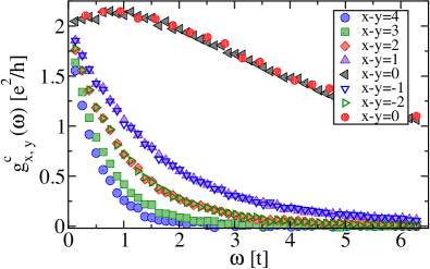
Figure 2: (Color online) The charge conductance $g^{c}_{x,y}(\omega_{n})$ for a noninteracting chain of spinful fermions with length $L=200$, periodic boundary conditions, and inverse temperature $\beta t=50$. Results for different distances $x-y$ between the perturbation and the measurement are displayed, for $x-y=0$ results are also shown for $\beta t=20$ (red circles). They all extrapolate in the $\omega\to 0$ limit to a conductance of $g^{c}_{x,y}(\omega\to 0)\to 2e^{2}/h$ as expected, see main text. The errors in the data are smaller than the point size.

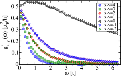
Figure 3: (Color online) The spin conductance $g^{s}_{x,y}(\omega_{n})$ for the same system and parameters as in Fig. 2. All curves extrapolate in the $\omega\to 0$ limit to the theoretically expected ideal conductance of $g^{s}_{x,y}(\omega\to 0)\to 0.5\mu_{B}^{2}/h$. As for Fig. 2 the errors are smaller than the point size.

Independent of the distance $x-y$ between the perturbation and the response all curves have the same direct current (d.c.), i.e. $\omega\rightarrow 0$, limit. Furthermore we can see that the conductances at finite frequencies only depend on the absolute value $|x-y|$. Thus we extrapolate the curves for different distances $|x-y|$ and average their $g^{\nu}(\omega=0)$ values in order to obtain the d.c. conductance, $g^{\nu}$. For the extrapolation we use a polynomial fit of degree six, $g^{\nu}_{x,y}(\omega_{n})=g^{\nu}(\omega=0)+\sum_{i=1}^{6}C_{i}\omega_{n}^{i}$. The fitting procedure and the differences in $g^{\nu}(\omega=0)$ for the different distances $|x-y|$ give an estimate for the error of the numerically obtained d.c. conductance. It is important to stress that the errors are completely dominated by the extrapolations. The statistical errors of the simulations at frequencies $\omega_{n}$ are very small and have almost no influence on the extrapolated value for the d.c. conductance. Note also that we can only provide a sensible error estimate. The true error is unknown and might in some cases be larger than the estimated error.

In order to ensure the junctions behave independently of each other we require $T\gg u/L$ to be satisfied. In this case the simulation results remain independent of length, so that no additional finite size scaling is required. Therefore, the systematic extrapolation to a vanishing Matsubara frequency will give results in the thermodynamic limit.

When we run our simulations at higher temperatures the Matsubara frequencies are further apart from each other, see Fig. 2, which makes the extrapolation to the zero frequency limit more difficult. On the other hand, since SSE is a high temperature expansion, lower temperatures will increase the simulation time, especially because in our case measurements of imaginary time correlation functions are necessary for all $\tau$, and we will require larger system lengths to satisfy $T\gg u/L$. It turns out that $\beta t=50$ is a good compromise between reasonable simulation times and a good accuracy of the extrapolation $\omega\to 0$. As expected for a non-interacting system the d.c. conductance is perfect, i.e. we find $2e^{2}/h$ for the charge conductance, since we have two independent charge channels ($\sigma=\uparrow,\downarrow$), see Fig. 2. Similarly we find $0.5\mu_{\text{B}}^{2}/h$ for the spin conductance consistent with the spin being $1/2$ in units of $\mu_{\text{B}}$, see Fig. 3.

Next, we consider the homogeneous interacting Hubbard model which is integrable by Bethe ansatz. In particular, the Luttinger liquid (LL) parameters $K_{\nu}$ as well as the spin and charge velocities $u_{\nu}$ of the elementary excitations can be determined exactly.Essler et al. (2005) For the conductances and compressibilities one finds, in particular,Shirakawa and Jeckelmann (2009); Sano and Ōno (2004); Giamarchi (2004); Essler et al. (2005)

$$\kappa_{\nu} = \frac{2K_{\nu}}{\pi u_{\nu}}\,,\,\,g^{c}=\frac{2e^{2}}{h}K_{c}\,,\textrm{ and}\,\,g^{s}=\frac{\mu_{\text{B}}^{2}}{2h}K_{s}\,.$$ (6)

We are considering here only the $SU(2)$ symmetric case where the spin LL parameter is fixed, $K_{s}=1$. In Fig. 4(a) we show a comparison between the QMC result for the charge conductance at fixed chemical potential $\mu=t$ and various interaction strengths $U$ after extrapolating to the zero frequency limit and the Bethe ansatz result (6). To obtain the LL parameter $K_{c}$, an integral equation obtained by Bethe ansatzEssler et al. (2005) has been evaluated numerically.

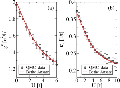
Figure 4: (Color online) Comparison between QMC data for the homogeneous Hubbard chain (I) with parameters $\mu=t$, $\beta t=50$, and $L=150$, and the exact Bethe ansatz results. Panel (a) shows the charge conductance, panel (b) the charge compressibility.

In Fig. 4(b) we show a similar comparison for the charge compressibility. The QMC data in Fig. 4 generally agree quite well with the exact results for all interaction strengths $U$.

For the half-filled case, $\mu_{j}=0$, it is known that the Hubbard model shows a Mott transition at arbitrarily small $U>0$ from a conducting to an insulating ground state. The charge gap $\Delta_{c}(U)$, measured in units of $t$, can be calculated by Bethe ansatz and is given byEssler et al. (2005)

$$\Delta_{c} = -2+\frac{U}{2}+2\int_{0}^{\infty}\frac{ds}{s}\frac{J_{1}(s)\exp(-sU/4)}{\cosh(sU/4)}$$ (7)

$$\approx \frac{4}{\pi}\sqrt{U}\exp\left(-\frac{2\pi}{U}\right)$$

where $J_{1}(s)$ is a Bessel function. The second line in Eq. (7) represents the result for small $U$ where the charge gap is exponentially small. For large $U$, the charge gap will scale linearly in the Hubbard interaction $U$. The spin channel, on the other hand, remains gapless, the spin conductance is independent of $U$, and the Luttinger parameter is fixed in the thermodynamic limit to $K_{s}=1$ due to the $SU(2)$ symmetry. In the QMC data shown in Fig. 5 the spin conductance is indeed close to $g^{s}=\mu_{B}^{2}/2h$. Note that for finite lengths $L$ there will be logarithmic corrections, $K_{s}\sim 1+1/\ln(L/L_{0})$ with a characteristic length scale $L_{0}$,Söffing et al. (2013) which might partly explain why the QMC data for the spin conductance are slightly larger than the thermodynamic limit result. For the charge conductance we find finite values for $U<2$ and values close to zero for $U>2$.

To understand these results it is important to stress that the QMC results are for finite chains of length $L=150$ at a finite temperature $T\gg u/L$. The charge gap $\Delta_{c}$ leads to a characteristic temperature scale $T_{c}\sim\Delta_{c}$ and we expect the conductance to scale as

$$g^{c}(T,U)=g^{c}_{0}\exp(-T_{c}/T)\,,$$ (8)

i.e. the conductance will only become zero for temperatures small compared to $\Delta_{c}$. We also require chain lengths which are large compared to $L_{c}(U)$, a characteristic length scale $L_{c}\sim 1/\Delta_{c}$, which will be satisfied due to the condition on the temperature and $T\gg u/L$. Since the charge gap is exponentially small for small $U$, very small temperatures are required to see the charge gap in the conductance. The numerical results are well described by setting $T_{c}\sim\Delta_{c}$ and using the small $U$ expansion for the charge gap given by Eq. (7).

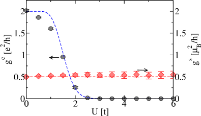
Figure 5: (Color online) The Hubbard chain at half-filling ($\mu=0$, $\beta t=50$, $L=150$). The charge conductance only drops slowly to zero because of the exponentially small charge gap at small $U$. The drop in $g^{c}$ is well described by Eq. (8) (blue dashed line). The spin conductance, on the other hand, is independent of $U$ and fixed by the $SU(2)$ symmetry (red dashed line).

So far we have concentrated on testing the QMC algorithm for homogeneous systems. As a next step, we consider a simple example for a noninteracting spinful inhomogeneous system where the QMC results can be directly compared to an analytical solution. As in all the inhomogeneous models discussed in the following we are considering a periodic chain of length $L$ with parameters as given in Table 1. Here we set $U_{\ell}=U_{w}=0$ while the hopping strengths are different, $t_{\ell}\neq t_{w}$. The transmission and reflection amplitudes for non-interacting spinless fermions are known in this case.Sedlmayr et al. (2014) Since the non-interacting Hubbard model has two independent spin channels, the reflection and transmission follows directly from the spinless result. The two velocities in the left and right part of the chain for each spin channel are given by

$$u_{\ell,w;\sigma}=2at_{\ell,w}\sin\left[ak_{\ell,w;\sigma}\right]\,,$$ (9)

where $k_{\ell,w;\sigma}=\frac{1}{a}\arccos{\frac{\mu_{\sigma}}{2t_{\ell,w}}}$ are the Fermi momenta in the lead and the wire, and $a$ is the lattice spacing. From this the reflection coefficient can be written as

$$R=-\frac{u_{\ell}-u_{w}}{u_{\ell}+u_{w}}$$ (10)

leading to a transmission

$$|T|^{2}=\left(1-|R|^{2}\right)\frac{u_{\ell}}{u_{w}}\,.$$ (11)

The conductance for each spin species is therefore given by $G=\left(1-|R|^{2}\right)e^{2}/h$ so that $g^{c}=2G$. An analogous calculation leads to $g^{s}=\left(1-|R|^{2}\right)\mu_{B}^{2}/2h$. These analytical results are shown as lines in Fig. 6 and compared to the QMC data.

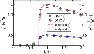
Figure 6: (Color online) QMC data for the charge and spin conductances of a junction of two non-interacting wires (symbols) with $t_{w}=t$, $\mu=1.5t$, $\beta t=50$, and $L=200$ compared to the exact result (lines).

	$-L/2\leq j<0$	$0\leq j<L/2$
$t_{j}$	$t_{\ell}=1$	$t_{w}$
$U_{j}$	$U_{\ell}=0$	$U_{w}>0$
$\mu_{j}$	$\mu_{\ell}$	$\mu_{w}$

Table 1: (Color online) The parameters of the inhomogeneous system.

As soon as both bands start to become filled the conductance increases drastically up to a maximum at the homogeneous point and then slowly drops down. The QMC results are in good agreement with the theoretical prediction.

III Spinless inhomogeneous fermion chains

Here we study the interacting spinless fermion model (I). Analytically, we have investigated this model already in two recent publications.Sedlmayr et al. (2012, 2014) Our main result was that there exists a line of non-trivial conducting fixed points where the backscattering at the junction vanishes despite the inhomogeneity of the system. In Ref. Sedlmayr et al., 2014 we have, in particular, been able to formulate a conformally invariant boundary theory which describes these fixed points. One prediction of this theory was that two different boundary Luttinger parameters exist which determine the scaling of autocorrelations in imaginary time at the boundary. We have been able to verify these scaling predictions numerically by quantum Monte Carlo simulations. Furthermore, we also obtained an analytic formula for the Friedel oscillationsFriedel (1958) in the density near the boundary which are known to have a characteristic amplitudeEgger and Grabert (1995); Eggert and Affleck (1995); Söffing et al. (2009) and give information about the interacting correlation functions and the strength of the backscattering.Sedlmayr et al. (2012, 2014); Rommer and Eggert (2000) However, at that time we have not been able to check the main prediction—the existence of a line of conducting fixed points—directly. The aim of this section is to provide such a direct check using the QMC method described in the previous section.

III.1 The half-filled case

The half-filled case, Eq. (I) with $\mu_{j}\equiv 0$, is the easiest to analyze for two reasons. First, the homogeneous spinless fermion model is integrable for all interaction strengths $U_{j}\equiv U$ and chemical potentials $\mu_{j}\equiv\mu$. However, only for $\mu=0$ (density $\langle n_{j}\rangle=1/2$) can the velocity of the elementary excitations $u$ and the Luttinger liquid parameter $K$ be determined in closed form

$$u=at\pi\frac{\sqrt{1-(U/2)^{2}}}{\arccos(U/2)},\quad K=\frac{\pi}{2[\pi-\arccos(U/2)]}\,.$$ (12)

These results are valid in the critical regime $-2<U\leq 2$ where the low-energy properties of the model are described by Luttinger liquid theory. Second, we found in Ref. Sedlmayr et al., 2012 that also the criterion for perfect conductance at an abrupt junction is particularly simple in this case. In general, each local perturbation in the chain leads to an oscillating backscattering $\sim\lambda\textrm{e}^{-\mathrm{i}2k_{F}x}\Psi_{+}^{\dagger}\Psi_{-}$ where $\Psi_{\pm}$ are the left- and right-moving fermion fields and $k_{F}$ is the Fermi wavenumber with $k_{F}=\pi/2$ in the half-filled case. The scattering amplitude $\lambda$ in the half-filled case takes the simple form

$$\lambda\propto\sum_{j}\textrm{e}^{-\mathrm{i}2k_{F}j}(u_{j+1}-u_{j})\,.$$ (13)

While this amplitude averages to zero in the bulk of the lead and the bulk of the wire, it is nonzero exactly at the boundary with

$$\lambda\propto u_{\ell}-u_{w}\,.$$ (14)

For all interaction strengths in the critical regime we therefore obtain a powerful and simple prediction for perfect conductance, i.e., conductance across a junction without any backscattering: The conductance is perfect if the velocity of excitations in the lead $u_{\ell}$ exactly matches the velocity of excitations $u_{w}$ in the interacting quantum wire. If the condition (14) is fulfilled, then the conductance across a junction of a semi-infinite wire with LL parameter $K_{\ell}$ and a semi-infinite wire with LL parameter $K_{w}$ is given bySedlmayr et al. (2012, 2014)

$$G=\frac{e^{2}}{h}\bar{K}\quad\mbox{with}\quad\bar{K}=\frac{2K_{\ell}K_{w}}{K_{\ell}+K_{w}}\,.$$ (15)

For a noninteracting lead this reduces to $\bar{K}=2K_{w}/(1+K_{w})$. In Fig. 7 we provide a numerical test of this prediction comparing the conductance from QMC with the theoretically predicted value for ideal conductance (15) if $u_{\ell}=u_{w}$.

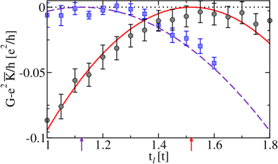
Figure 7: (Color online) Comparison between QMC data (symbols) for the inhomogeneous spinless chain (I) with parameters $\mu=0$, $t_{w}=t$, $U_{\ell}=0$, $\beta t=50$, $U_{w}=1.8t$ (black), $U_{w}=0.4t$ (blue) and $L=400$, and the analytical expression, Eq. (16) (solid red line and dashed purple line) with $\alpha$ a fitting parameter. The dotted line shows perfect conductance $\bar{K}e^{2}/h$, Eq. (15), with $\bar{K}\approx 0.739$ and $\bar{K}\approx 0.940$ respectively. The arrows at the $t_{\ell}$-axes indicate the points $u_{\ell}=u_{w}$.

Furthermore, we show that the conductance away from the fixed point is well fitted by the second order perturbative result

$$G(T)=\frac{e^{2}}{h}\left[\bar{K}-\underbrace{\alpha(u_{\ell}-u_{w})^{2}}_{\lambda^{2}}\left(\frac{T}{T_{K}}\right)^{2\bar{K}-2}\right]$$ (16)

where the amplitude $\alpha$ is a free parameter. Note that for repulsive interactions, $K_{w}<1$, backscattering is always relevant and increases in the limit $T\to 0$. The conductance curve shown in Fig. 7 is then expected to become singular and will approach zero everywhere except at the conducting fixed point.

III.2 Away from half-filling

Next, we want to study the conductance in the spinless fermion model (I) with a constant but nonzero chemical potential, $\mu_{j}\equiv\mu\neq 0$. In this case, the condition $u_{\ell}=u_{w}$ for perfect conductance across a junction no longer holds. Instead, we can calculate the backscattering amplitude $\lambda$ only to lowest order in the interaction and findSedlmayr et al. (2014)

$$\lambda \approx \frac{a}{2\pi}\left(\frac{t_{\ell}}{\sin[ak_{F\ell}]}+\frac{U_{\ell}}{\pi}-\frac{t_{w}}{\sin[ak_{Fw}]}-\frac{U_{w}}{\pi}\right)$$ (17)

$$-\frac{a\mu}{4\pi}\left(\cot[ak_{F\ell}]-\cot[ak_{Fw}]\right)\,.$$

Surprisingly, the scattering amplitude in lowest order is real. Numerically, we have found that this seems to be the case even for strong interactions. As a consequence, it should still always be possible to find a conducting fixed point. Eq. (16) continues to describe the scaling of the conductance if the proper backscattering amplitude is used. The LL parameter $K_{w}$ for the interacting wire can no longer be written down in closed form. However, it is possible to determine $K_{w}$ to high accuracy by numerically solving integral equations obtained by Bethe ansatz.Essler et al. (2005) In a previous paper, Ref. Sedlmayr et al., 2014, we have shown that for every chemical potential $\mu$ it is possible to induce a sign change in the Friedel oscillations near the junction by tuning the parameters of the lead and wire. Since the Friedel oscillations are linear in the backscattering amplitude $\lambda$ (see Ref. Sedlmayr et al., 2014 and Sec. IV) this shows that one can change the sign of $\lambda$ thus providing an indirect proof for a conducting fixed point where $\lambda=0$.

Here we want to show the existence of conducting fixed points away from half-filling directly. In Fig. 8 we present QMC data for the conductance across a junction of a lead and an interacting quantum wire for various spatially constant chemical potentials.

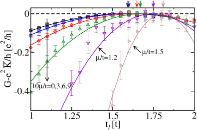
Figure 8: (Color online) Conductance $G-\bar{K}e^{2}/h$ for the inhomogeneous spinless chain (I) with parameters $t_{w}=t$, $U_{w}=1.8t$, $U_{\ell}=0$, $\beta t=50$, and $L=400$, for different chemical potentials $\mu$. The density varies between $n\approx 0.51$ ($\mu/t=0.1$) and $n\approx 0.75$ ($\mu/t=1.5$). The dashed line indicates perfect conductance. The solid lines show fits to $-A(u_{\ell}-B)^{2}$ with $A$ and $B$ fitting parameters, see Eq. (17), the most general correction consistent with the model. The arrows indicate the points when $u_{\ell}=B$.

Note that we plot the measured conductance $G$ minus the ideal conductance without backscattering given by $\bar{K}e^{2}/h$, i.e. the zero line in the plot indicates perfect conductance where backscattering at the junction is absent. For all chemical potentials shown, the curves indicate the existence of a perfectly conducting fixed point. As expected based on the lowest order result of the backscattering amplitude, Eq. (17), the position of the fixed point shifts as a function of chemical potential.

IV The inhomogeneous Hubbard model

While the spinless case is the easiest to analyze theoretically and nicely demonstrates the existence of nontrivial perfectly conducting fixed points for abrupt lead-wire junctions, its value as a realistic model to describe experiments on quantum wires is limited. While one could potentially spin polarize electrons in strong magnetic fields making them effectively spinless, the typical experimental setup will involve spinful electrons. As a next step, we therefore want to generalize the investigation of perfectly conducting fixed point to the Hubbard model (I). We will concentrate here on the experimentally most common case without magnetic fields $B_{j}\equiv 0$. The Hubbard model then possesses a $SU(2)$-spin symmetry which fixes the spin Luttinger liquid parameter to $K_{s}\equiv 1$.

In the following we will first present the low-energy effective theory for an inhomogeneous Hubbard chain and then compare this theory with QMC data for the conductances across a lead-wire junction.

IV.1 Luttinger liquid theory

The homogeneous Hubbard model at low energies in the critical regime where both spin- and charge excitations are gapless can be described by an effective quadratic bosonic theory, the Luttinger liquid. In the following we assume that we can generalize this effective theory directly to the inhomogeneous case. Such an approach where only a narrow band of states near the Fermi momenta are kept is certainly justified if the hopping and interaction parameters as well as the chemical potentials in lead and wire are close enough so that backscattering is weak and only states close to the Fermi momenta will be mixed. In the following, we implicitly assume that we are in such a limit. For large inhomogeneities at the junctions only numerical data can clarify if the Luttinger liquid theory results still holds qualitatively.

The lead-wire junction at low energies is described by the effective Hamiltonian $H=H_{\rm q}+H_{\rm bs}$ (see App. A for details) where

$$H_{\rm q}=\frac{1}{2}\int\,\mathrm{d}x\sum_{\nu=c,s}\left(\frac{u^{\nu}_{x}}{K^{\nu}_{x}}(\partial_{x}\phi_{i})^{2}+u^{\nu}_{x}K^{\nu}_{x}(\partial_{x}{\tilde{\phi}}_{i})^{2}\right)\,$$ (18)

describes the bosonic modes which obey the commutation relations $[\phi_{\nu}(x),\Pi_{\eta}(x^{\prime})]=\mathrm{i}\delta_{\nu\eta}\delta(x-x^{\prime})$ for $\nu,\eta=c,s$ with $\Pi_{\nu}(x)=\partial_{x}\tilde{\phi}_{\nu}(x)$ a conjugate momentum. The spin ($\nu=s$) and charge ($\nu=c$) velocities and Luttinger parameters, $u^{\nu}_{x}$ and $K^{\nu}_{x}$, respectively completely characterize the systems low energy properties. We focus again on the case of a sharp jump where we have two different regions with $u^{\nu}_{x<0}=u^{\nu}_{\ell}$ and $u^{\nu}_{x>0}=u^{\nu}_{w}$. Provided the two boundaries of the wire are far enough apart this is sufficient to characterize the required properties of the system.

Additionally we have local backscattering terms at the junctions,

$$H_{\rm bs} \approx \lambda_{R}\cos[\sqrt{2\pi}\phi_{c}(0)]\cos[\sqrt{2\pi}\phi_{s}(0)]$$

$$+\lambda_{I}\sin[\sqrt{2\pi}\phi_{c}(0)]\cos[\sqrt{2\pi}\phi_{s}(0)]\,.$$

Here $\lambda_{R}$ denotes the real part and $\lambda_{I}$ the imaginary part of the scattering amplitude. Note that the $\sin[\sqrt{2\pi}\phi_{s}(0)]$ term is forbidden by the $SU(2)$ symmetry in the case without magnetic fields which is considered here. To lowest order in the interaction one can calculate the backscattering coefficients and we find

$$\lambda_{R} = \frac{1}{\pi}\left(\frac{v^{1}_{\ell}}{\sin^{2}[ak_{F\ell}]}-\frac{v^{1}_{w}}{\sin^{2}[ak_{Fw}]}-\frac{2aU_{\ell}}{\pi}+\frac{2aU_{w}}{\pi}\right.$$ (20)

$$\quad+a\mu_{\ell}\cot[ak_{F\ell}]-a\mu_{w}\cot[ak_{Fw}]\bigg{)}\,\textrm{, and}$$

$$\lambda_{I} = \frac{2aU_{\ell}}{\pi^{2}}\cot[ak_{F\ell}]-\frac{2aU_{w}}{\pi^{2}}\cot[ak_{Fw}]$$

with $v^{1}_{\ell,w}$ being renormalized Fermi velocities defined in App. A, and $k_{F\ell,w}$ being the Fermi momenta in the lead and the wire, respectively. This result generalizes Eq. (17) to the spinful case. Importantly, the scattering amplitude $\lambda$ is no longer real. This means that now, in general, two separate conditions have to be fulfilled to make the backscattering amplitude zero. Here we want to concentrate on a non-interacting lead, $U_{\ell}=0$. In this case the imaginary part of the backscattering amplitude is given by $\lambda_{I}\sim U_{w}\cot[k_{Fw}a]$. In order for $\lambda_{I}$ to vanish either (i) $U_{w}=0$ or (ii) $\cos[k_{Fw}a]=0$. The first case is not of interest to us and leads for $\mu_{\ell}=\mu_{w}$ to the trivial fixed point of a non-interacting homogeneous system. The second possibility implies that the wire is half-filled, $k_{Fw}=\pi/2$ and $\mu_{w}=0$. Then Eq. (20) implies that one can find a point where $\lambda_{R}=0$ for any set of hopping and interaction wire parameters, $t_{w}$ and $U_{w}$. This would make the backscattering in the half-filled inhomogeneous Hubbard model analogous to the spinless case considered before. However, even in the absence of backscattering at the junction, the umklapp scattering term

$$H_{U}\sim U\int\,\mathrm{d}x\cos(\sqrt{8\pi}\phi_{c}(x))$$ (21)

is non-oscillating and relevant for repulsive interactions leading to the charge gap (7) at half-filling. Therefore only the spin sector can show ideal conductance at a non-trivial fixed point for half-filling. Note that for attractive interactions the charge sector remains gapless while a gap develops in the spin sector. In this case, $K_{w}^{c}>1$ so that backscattering at the junction is always irrelevant leading to perfect charge conductance. Away from half-filling, on the other hand, Eq. (20) suggests that non-trivial conducting fixed points do not exist at all. However, it is important to stress that this analysis is based on an expansion of the scattering amplitude to lowest order in the Hubbard interaction. Only numerical calculations can clarify if this result also holds qualitatively for strong inhomogeneities.

The calculation of the conductance in a lead-wire-lead Hubbard system for weak backscattering is a straightforward generalization of the result in the spinless case, Eq. (16). In the model considered here the only backscattering present is the $2k_{F}$ spin-conserving backscattering given by Eq. (IV.1) in bosonized form. In general, also other sources of backscattering—including processes which include a spin flip—can be present at the boundary which could lead to different backscattering amplitudes for charge and spin. The change of the conductance as a function of temperature (energy scale) is determined by the scaling dimension of the boundary operator. This scaling dimension is found from the renormalization group (RG) equation

$$\frac{1}{\lambda}\frac{\,\mathrm{d}\lambda}{\,\mathrm{d}\ln T}=\bar{K}_{c}/2+\bar{K}_{s}/2-1\,,$$ (22)

where

$$\frac{1}{\bar{K}_{\nu}}=\frac{1}{2}\left[\frac{1}{K^{\nu}_{\ell}}+\frac{1}{K^{\nu}_{w}}\right]\,,$$ (23)

and

$$\frac{1}{\bar{u}_{\nu}}=\frac{1}{2}\left[\frac{1}{u^{\nu}_{\ell}}+\frac{1}{u^{\nu}_{w}}\right]\,,$$ (24)

with $\nu=c,s$. For a lead-wire system, i.e., a single junction between a lead and a wire the ideal conductance in the absence of backscattering now reads

$$g_{0}^{c,s}=\frac{2K_{\ell}^{c,s}K_{w}^{c,s}}{K_{\ell}^{c,s}+K_{w}^{c,s}}\left\{\begin{array}[]{cc}2\frac{e^{2}}{h}&\textrm{ for charge,}\\ &\\ \frac{\mu_{B}^{2}}{2h}&\textrm{ for spin,}\end{array}\right.$$ (25)

where again $K^{s}_{\ell}=K^{s}_{w}\equiv 1$ for $SU(2)$ invariant models, although finite size and temperature can give significant logarithmic corrections.Söffing et al. (2013) Finally one finds for the differential conductanceFurusaki and Nagaosa (1996)

$$g^{c,s}=g_{0}^{c,s}-\alpha_{c,s}\left(\frac{|\lambda|}{\bar{u}_{c,s}}\right)^{2}\left(\frac{T}{T_{K}}\right)^{\bar{K}_{c}+\bar{K_{s}}-2}\,,$$ (26)

where $T_{K}$ is the characteristic temperature scale set by the backscattering strength and $\alpha_{c,s}$ are constants.

IV.2 Conductances from QMC

As for the spinless case we will, in the following, use the SSE code to calculate the conductances across an abrupt lead-wire junction described by the inhomogeneous Hubbard model (I). Based on the analysis of the lowest order result for the backscattering amplitude (20) we might expect that the half-filled, particle-hole symmetric case is different from any other generic filling. We will therefore discuss this case separately.

IV.2.1 The half-filled case

For half-filling the backscattering amplitude (20) to lowest order in the Hubbard interaction is real. If this also holds for stronger interactions then we might expect to be able to find a non-trivial conducting fixed point for any set of wire parameters by changing the hopping $t_{\ell}$ in the non-interacting lead. At this fixed point we expect ideal spin conductance while the charge conductance will become zero in the thermodynamic limit due to the relevant umklapp scattering term in the bulk, Eq. (21). In Fig. 9 we exemplary show results for the case $U_{w}=1$.

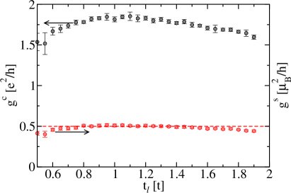
Figure 9: (Color online) Charge and spin conductance for the inhomogeneous half-filled Hubbard model for a chain with $L=150$, $t_{w}=t$, $\beta t=25$, and $U_{w}/t=1$. We find ideal spin conductance for $t_{\ell}\approx 1$.

The spin conductance indeed reaches its ideal value $g^{s}=\mu_{B}^{2}/2h$ in a region around $t_{\ell}\approx 1$. The maximum is, however, quite broad so that it is not possible to determine the fixed point precisely. The charge conductance also shows a maximum in the same region. Similar to the homogeneous case shown in Fig. 5 the conductance is nonzero only because the temperature in the numerical simulations is large compared to the exponentially small charge gap (7). In the low-temperature limit, the charge conductance will vanish for all hopping parameters $t_{\ell}$.

IV.2.2 Away from half-filling

Away from half-filling the analysis of the lowest order result for the scattering amplitude suggests that non-trivial conducting fixed points do not exist. Checking all possible parameter combinations in the lead and in the wire numerically is not feasible, so this statement cannot be explicitly shown. However, it is possible to numerically test several different cases by keeping the parameters in the non-interacting lead fixed and vary both interaction and hopping strength in the wire. Here the density across the junction is kept constant at a generic value $n=1/4$ by choosing the chemical potentials $\mu_{\ell}$ and $\mu_{w}$ accordingly. In Figs. 10 and 11 we plot the relative conductances $g_{\lambda}^{c,s}=g^{c,s}-g_{0}^{c,s}$ so that $g_{\lambda}^{c,s}=0$ would correspond to a conducting fixed point. Note that we vary $t_{w}$ here so that the Luttinger parameter $K_{w}^{c}$ and therefore $g_{0}^{c}$ is different for each point shown in Figs. 10 and 11.

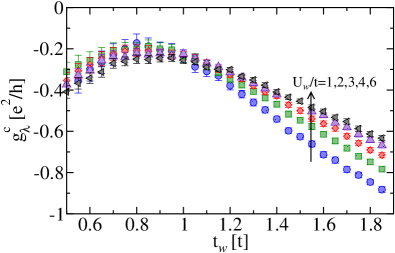
Figure 10: (Color online) Relative differential charge conductance $g_{\lambda}^{c}=g^{c}-g_{0}^{c}$ for different values of $U_{w}$ as a function of $t_{w}$ in an inhomogeneous system of length $L=150$ with $t_{\ell}=t$, $\beta t=25$ and constant filling $n=1/4$ along the chain.

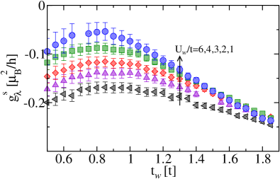
Figure 11: (Color online) Relative differential spin conductance $g_{\lambda}^{s}=g^{s}-g_{0}^{s}$ for different values of $U_{w}$ as a function of $t_{w}$ in an inhomogeneous system of length $L=150$ with $t_{\ell}=t$, $\beta t=25$ and constant filling $n=1/4$ along the chain.

For both the spin and the charge conductance we see that the value for ideal conductance $g_{\lambda}^{c,s}=0$ is never reached. This is in contrast to the spinless case in Fig. 8, where for a given value on one side it was possible to achieve perfect conductance by just varying a single parameter on the other side. While this does not prove the conjecture—based on the lowest order results for the scattering amplitude—that non-trivial conducting fixed point do not exist in the spinful case away from half-filling, it shows that the spinful case is different from the spinless case.

IV.3 Friedel oscillations

The inhomogeneity at a lead-wire junction leads to Friedel oscillations in the local density which are proportional to the backscattering amplitude $\lambda$.Sedlmayr et al. (2012, 2014); Rommer and Eggert (2000) Calculating these oscillations for small inhomogeneities by field theory and comparing the results with QMC data is therefore an alternative way to study backscattering at the junction. In Ref. Sedlmayr et al., 2014 we have shown that such an analysis can be used to find conducting fixed points in the spinless case. In the following, we will generalize the field theory for the Friedel oscillations to the spinful case and exemplary compare the result with numerical data.

The bosonized density operator for spinful fermions is given by

$$n(x) = n_{0}(x)-\frac{1}{\sqrt{\pi}}\partial_{x}\phi_{c}(x)$$

$$+\frac{\textrm{const.}}{\pi a}\sin[2k_{Fx}^{*}x+\sqrt{2\pi}\phi_{c}(x)]\cos[\sqrt{2\pi}\phi_{s}(x)]\,.$$

The oscillating contribution to the density is therefore obtained by the following expectation value

$$\rho_{\rm alt}(x)\propto\left\langle\sin[2k_{Fx}^{*}x+\sqrt{2\pi}\phi_{c}(x)]\cos[\sqrt{2\pi}\phi_{s}(x)]\right\rangle$$ (27)

which has to be calculated with the full bosonized Hamiltonian including the backscattering term. Here $k_{Fx}^{*}$ is the Fermi momentum which can be found in the grand canonical setting from the bulk density $\rho_{x}\equiv\langle n_{0}(x)\rangle=k_{Fx}^{*}/\pi$ which is temperature dependent. In the following we will calculate the Friedel oscillations (27) to first order in the effective backscattering coefficient $\lambda$. For this we require the following integral:

$$\tau(x) \equiv 4\int_{0}^{\beta}\,\mathrm{d}\tau\prod_{\nu=c,s}\left\langle\textrm{e}^{\mathrm{i}\sqrt{2\pi}\left[\phi_{\nu}(x,0)-\phi_{\nu}(0,\tau)\right]}\right\rangle$$ (28)

$$= \int_{0}^{\beta}\,\mathrm{d}\tau\prod_{\nu=c,s}\textrm{e}^{\pi\left[G_{\nu}(x,0;\tau)-G_{\nu}(0,0;0)\right]}\,.$$

The Green’s function $G_{i}(x,y,\tau)$ is defined in Appendix B and can be obtained as a direct generalization of the spinless case, see Ref. Sedlmayr et al., 2014. Note that in the spinful case the integral consists of a product of a spin and a charge vertex operator correlation function and can therefore no longer be evaluated exactly. The integral can be cast into the following form

$$\tau(x) = \prod_{\nu=c,s}\left(\frac{4\pi Ta}{u^{\nu}_{x}}\right)^{\frac{\bar{K}_{\nu}}{2}}\left(\frac{u^{\nu}_{x}}{2\pi aT}\sinh\left[\frac{2\pi Tx}{u^{\nu}_{x}}\right]\right)^{-\frac{K^{\nu}_{x}}{2}}$$ (29)

$$\times\int_{0}^{\pi}\frac{\,\mathrm{d}y}{\pi T}\prod_{\nu=c,s}\left[z_{\nu}+\sqrt{z_{\nu}^{2}-1}\cos[y]\right]^{-\frac{\bar{K}_{\nu}}{2}}\,,$$

with

$$z_{\nu}\equiv\coth\left[\frac{2\pi Tx}{u^{\nu}_{x}}\right]\,.$$ (30)

The final result for the Friedel oscillations to first order in the backscattering is

$$\rho_{\rm alt}(x)\propto-\big{[}\lambda_{R}\sin[2k_{Fx}^{*}x]+\lambda_{I}\cos[2k_{Fx}^{*}x]\big{]}\tau(x)\,.$$ (31)

In Fig. 12 we compare the field theory formula (31) with QMC results for the local density near the boundaries of a lead-wire junction.

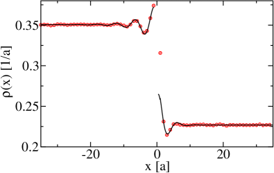
Figure 12: (Color online) Local density at a lead-wire junction. Symbols denote the QMC results, the solid line denotes the Luttinger liquid result formula (31). The numerical data are obtained for an inhomogeneous Hubbard model with length $L=150$, hoppings $t_{\ell}=t$, $t_{w}=0.8t$, wire interaction $U_{w}=2t$, and inverse temperature $\beta t_{w}=25$. The chemical potentials are $\mu_{\ell}=1.7t$, $\mu_{w}=1.7t$. Error bars for the QMC data are smaller than the symbols.

Sites with $x<0$ represent the non-interacting lead, sites with $x>0$ the interacting quantum wire. The bulk densities in the bulk of the lead and the wire can be calculated by Bethe ansatz and are consistent with the numerical data. To fit the alternating part of the local density, both the position of the scattering center as well as the amplitude of the oscillations are used as fitting parameters. The obtained fit describes the data very well, showing that the field theory description of the inhomogeneous system is working although the inhomogeneity in the considered example is not small. A more detailed study of the Friedel oscillations across the full parameter space of the inhomogeneous Hubbard model (I) can, in principle, be used to search for conducting fixed points. Similar to the conductance, however, it is nearly impossible to show that non-trivial conducting fixed points do not exist away from half-filling because of the large parameter space which needs to be covered.

V Conclusions

Quantum wires—electrically conducting wires with diameters in the nanometer range in which quantum effects strongly influence the transport properties—offer insights into fundamental questions of many-body physics as well as possible avenues to new electronic devices. It is therefore important to develop numerical and analytical tools to investigate the properties of such systems.

In this paper we have studied, in particular, the simplest quantum wire device: an interacting quantum wire contacted by non-interacting leads. Contrary to most previous studies, we model the lead-wire junction microscopically and include electron scattering at the junction. The latter is ignored in the most commonly used field theoretical description of this setup where the junctions between leads and quantum wire are assumed to be perfectly adiabatic. Our microscopic approach starts from the opposite limit of a sharp junction leading to models of inhomogeneous tight-binding chains where parameters such as the hopping amplitude, the chemical potential, and the screened Coulomb interactions abruptly change on the scale of the lattice spacing.

To numerically investigate lead-wire junctions we have generalized a quantum Monte Carlo algorithm based on the stochastic series expansion technique which has been used previously for homogeneous systems.Louis and Gros (2003) This method allows us to calculate response functions in imaginary time. We calculate the linear response to an infinitesimal drop in electric or magnetic field. After a Fourier transformation to discrete Matsubara frequencies we have shown that at sufficiently low temperatures a reliable extrapolation to zero frequency is possible, giving access to the charge and spin conductance near zero temperature. To test the validity and accuracy of this approach we have studied different homogeneous and inhomogeneous setups where the conductances are known exactly. In all those test cases we have found very good agreement of the numerical data with the exact results, establishing this method as a reliable tool to study quantum wire devices.

As a first application, we have studied the conductance across a lead-wire junction in a spinless fermion system. In two previous publications,Sedlmayr et al. (2012, 2014) we have predicted by field theoretical means that non-trivial perfectly conducting fixed points exist despite the inhomogeneity of the system on the scale of the lattice spacing. At these fixed points the amplitude of the relevant backscattering process exactly vanishes. For the half-filled spinless fermion system we have predicted this to happen when the velocities of the excitations in lead and wire exactly match. Previously, we have only been able to provide indirect numerical evidence for this fixed point by studying Friedel oscillations and autocorrelations near the junction. Here we have directly calculated the conductance and shown that the result near the fixed point can be well fitted by the field theory formula requiring only a single fitting parameter. Next, we have also studied the conductance in inhomogeneous spinless fermion wires away from half-filling. In this case, field theory predicts that conducting fixed points still exist, however, the condition for perfect conductance is no longer a simple velocity matching. We have verified this prediction here numerically as well; values close to perfect conductance are obtained for all fillings investigated.

While spinless fermions are easiest to study by field theory, the spinful case is the experimentally more relevant one. To study whether or not non-trivial conducting fixed points still exist once the spin degree of freedom is included we have analyzed the inhomogeneous Hubbard chain without magnetic field using bosonization. This analysis provided evidence for a fundamental difference to the spinless case: while the amplitude of the relevant backscattering process is always real for spinless fermions it is complex, in general, for the spinful case. For the $SU(2)$ symmetric inhomogeneous Hubbard chain, in particular, we find to lowest order in the Hubbard interaction that the imaginary part of the backscattering amplitude only vanishes at half-filling (particle-hole symmetric case). If we conjecture that this holds to all orders in the interaction, then non-trivial conducting fixed points only exist for the half-filled system. Numerically, we have been able to show the existence of a conducting fixed point at half-filling for the inhomogeneous Hubbard model where the spin conductance takes it ideal value $\mu_{B}^{2}/2h$ while the charge conductance will vanish in the thermodynamic limit due to the charge gap induced for repulsive interactions by a relevant bulk umklapp scattering term. On the other hand, a non-trivial fixed point was not found for several lead-wire setups away from half-filling.

There seem to be therefore two main setups in which these conducting fixed points—described by a rather unusual boundary conformal field theorySedlmayr et al. (2014)—can possibly be investigated experimentally. On the one hand, one might consider a quantum wire of spin polarized electrons which is effectively described by a spinless fermion model. On the other hand, it might be possible to use a spinful quantum wire with a low-energy band structure which can be tuned to a particle-hole symmetric filling by a gate electrode. In both cases the field theory predicts that for a sufficiently sharp junction a non-trivial conducting fixed point should be accessible by tuning the effective bandwidths and chemical potentials of the leads. For the half-filled spinful model, in particular, a fixed point with perfect spin conductance can be found for repulsive interactions while perfect charge conductance is expected for attractive interactions with backscattering at the junction being always irrelevant in the latter case.

Finally, we note that the experiment described in Ref. KamataKumada et al., 2014 has recently been analyzed using the bosonic model (18) but without the local backscattering term (IV.1).Perfetto et al. (2014); Calzona et al. (2015) In these studies the authors find backscattering of a wavepacket injected into the lead at a lead-wire junction. We want to stress that this result is not in contradiction to the results presented here. While a wavepacket is indeed scattered at the junction in an inhomogeneous Luttinger model (18) even without a single electron backscattering term (IV.1) being present, the conductance will be ideal in this case as has already been stressed in Ref. Safi and Schulz, 1995.

Appendix A Luttinger liquid theory

The low energy behavior of the Hamiltonian, Eq. (I), can be described as a Luttinger liquid.Giamarchi (2004) Here we extend our analysis to a broader class of interactions that also includes the nearest neighbor interactions $V_{j,j+1}$. We will set $\hbar=1$ everywhere in this appendix. The interacting Hamiltonian now reads

$$H_{I} = \sum_{j,\sigma\sigma^{\prime}}\bigg{[}U_{j}:\psi^{\dagger}_{\sigma j}\psi_{\sigma j}::\psi^{\dagger}_{\sigma^{\prime}j}\psi_{\sigma^{\prime}j}:$$

$$\qquad+V_{j,j+1}:\psi^{\dagger}_{\sigma j}\psi_{\sigma j}::\psi^{\dagger}_{\sigma^{\prime}j+1}\psi_{\sigma^{\prime}j+1}:\bigg{]}\,.$$

Normal ordered operators are given by $:\psi^{\dagger}_{j}\psi_{j}:=\psi^{\dagger}_{j}\psi_{j}-\langle 0|\psi^{\dagger}_{j}\psi_{j}|0\rangle$, with $|0\rangle$ the ground state. To simplify matters we consider a spin-independent, $SU(2)$ symmetric interaction. The low-energy theory does however remain valid for a spin-dependent interaction provided the interaction is spin conserving. The derivation of the spatially inhomogeneous Luttinger liquid theory follows closely the standard homogeneous derivationSafi and Schulz (1995); Maslov and Stone (1995) but special care must be taken to include the local scattering at the boundary.Sedlmayr et al. (2012, 2014)

We assume that we can linearize the dispersion near the Fermi momenta $k_{Fx}$ into left and right moving particles via the ansatz

$$\frac{\psi_{\sigma j}}{\sqrt{a}}=\psi_{\sigma}(x)=\sum_{\alpha=\pm}\textrm{e}^{\mathrm{i}\alpha k_{Fx}x}\psi_{\sigma\alpha}(x)$$ (33)

where the Fermi momenta are given by

$$\mu_{x}=-2t_{x}\cos\left[ak_{Fx}\right]\,,$$ (34)

with $a$ the lattice spacing and $x=aj$. The $\alpha=+$ and $\alpha=-$ indices denote the right and left moving electrons respectively. After linearization we have for the noninteracting part of Eq. (I), taking the continuum limit,

$$H_{0} = -\int\,\mathrm{d}x\sum_{\alpha=\pm,\sigma}t_{x}\left[e^{\mathrm{i}ak_{Fx}}\psi^{\dagger}_{\sigma\alpha}(x)\partial_{x}\psi_{\sigma\alpha}(x)+\textrm{H.c.}\right]$$ (35)

$$-\int\,\mathrm{d}x\sum_{\alpha=\pm,\sigma}\left[2t_{x}e^{-i\alpha k_{Fx}(2x+a)}+\mu_{x}e^{-2\mathrm{i}\alpha k_{Fx}x}\right]$$

$$\qquad\times\psi^{\dagger}_{\sigma\alpha}(x)\psi_{\sigma\bar{\alpha}}(x)\,.$$

We have defined $\bar{\alpha}=-\alpha$. The contribution of the final two lines can be neglected in a homogeneous system, but will here still contribute near the boundary where $t_{x}$ and $\mu_{x}$ can sharply vary. Using Eq. 33 the interaction $H_{I}$ can be decomposed into parallel and perpendicular spin components, which in the usual nomenclatureGiamarchi (2004) are written as

$$H_{2} = \sum_{\sigma,\alpha}\int\,\mathrm{d}x\left[\frac{g^{2\perp}_{x}}{2}\rho_{\sigma\alpha}\rho_{\bar{\sigma}\bar{\alpha}}+\frac{g^{2\parallel}_{x}}{2}\rho_{\sigma\alpha}\rho_{\sigma\bar{\alpha}}\right],$$

$$H_{4} = \sum_{\sigma,\alpha}\int\,\mathrm{d}x\frac{g^{4}_{x}}{2}\rho_{\sigma\alpha}\rho_{\sigma\alpha}\,\textrm{, and}$$ (36)

$$H_{1} = \sum_{\sigma,\alpha}\int\,\mathrm{d}x\left[\frac{g^{1\perp}_{x}}{2}\psi^{\dagger}_{\sigma\alpha}\psi^{\dagger}_{\bar{\sigma}\bar{\alpha}}\psi_{\bar{\sigma}\alpha}\psi_{\sigma\bar{\alpha}}-\frac{g^{1\parallel}_{x}}{2}\rho_{\sigma\alpha}\rho_{\sigma\bar{\alpha}}\right]\,.$$

Here we have suppressed the spatial indices and defined the local right and left mover density $\rho_{\sigma\pm}=\psi^{\dagger}_{\sigma\pm}\psi_{\sigma\pm}$. Note that the $g^{1\parallel\sigma}_{x}$ process has been rewritten from its natural form to resemble a density-density interaction, however the final $g^{1\perp}$ process can not be formulated as a density-density interaction. It corresponds to a two particle backward scattering process. This is at best marginal, and will be neglected here. Umklapp scattering processes, when they are important, lead to a charge gap, these are discussed in the main text. In addition there are scattering terms in $H_{I}$ which originate with the inhomogeneity of the interaction which renormalize the backscattering in Eq. (35).Sedlmayr et al. (2012, 2014)

We introduce bosonic fields related to the particle density,

$$\rho_{\sigma\alpha}(x)=-\frac{1}{\sqrt{2\pi}}\partial_{x}\phi_{\sigma\alpha}\,,$$ (37)

which obey the commutation relations

$$\left[\phi_{\sigma\alpha}(x),\phi_{\sigma^{\prime}\alpha}(x^{\prime})\right] = -\frac{\mathrm{i}}{2}(\alpha\delta_{\sigma\sigma^{\prime}}\operatorname{sgn}(x-x^{\prime})+\mathrm{i}\sigma^{y}_{\sigma\sigma^{\prime}})\,\textrm{, and}$$

$$\left[\phi_{\sigma\alpha}(x),\phi_{\sigma^{\prime}\bar{\alpha}}(x^{\prime})\right] = -\frac{\mathrm{i}\alpha}{2}(\delta_{\sigma\sigma^{\prime}}+\mathrm{i}\sigma^{y}_{\sigma\sigma^{\prime}})\,.$$ (38)

The vertex operator is

$$\psi_{\sigma\alpha}(x)=\frac{1}{\sqrt{2\pi a}}e^{\mathrm{i}\alpha\sqrt{2\pi}[\phi_{\sigma\alpha}(x)]}\,.$$ (39)

The Hamiltonian can be reformulated as a quadratic Hamiltonian in these bosonic fields, $H_{\rm q}$, and local scattering terms $H_{\rm bs}$.

Firstly the quadratic part of the bosonic Hamiltonian is

$$H_{\rm q}=\frac{1}{8\pi}\int\,\mathrm{d}x\begin{pmatrix}\partial_{x}\phi_{\uparrow+}\\ \partial_{x}\phi_{\uparrow-}\\ \partial_{x}\phi_{\downarrow+}\\ \partial_{x}\phi_{\downarrow-}\end{pmatrix}^{T}\begin{pmatrix}4\pi v_{Fx}+2g^{4}_{x}&g^{2\parallel}_{x}-g^{1\parallel}_{x}&g^{4}_{x}&g^{2\perp}_{x}\\ g^{2\parallel}_{x}-g^{1\parallel}_{x}&4\pi v_{Fx}+2g^{4}_{x}&g^{2\perp}_{x}&g^{4}_{x}\\ g^{4}_{x}&g^{2\perp}_{x}&4\pi v_{Fx}+2g^{4}_{x}&g^{2\parallel}_{x}-g^{1\parallel}_{x}\\ g^{2\perp}_{x}&g^{4}_{x}&g^{2\parallel}_{x}-g^{1\parallel}_{x}&4\pi v_{Fx}+2g^{4}_{x}\end{pmatrix}\begin{pmatrix}\partial_{x}\phi_{\uparrow+}\\ \partial_{x}\phi_{\uparrow-}\\ \partial_{x}\phi_{\downarrow+}\\ \partial_{x}\phi_{\downarrow-}\end{pmatrix}\,.$$ (40)

The unrenormalized velocity is $v_{Fx}=2at_{x}\sin[ak_{Fx}]$. We make two unitary transformations which suffice to diagonalize $H_{\rm q}$. The first is $\phi_{\sigma\pm}=[\phi_{\sigma}\mp{\tilde{\phi}}_{\sigma}]/\sqrt{2}$. The new fields obey $[\phi_{\sigma}(x),\Pi_{\sigma^{\prime}}(x^{\prime})]=\mathrm{i}\delta_{\sigma\sigma^{\prime}}\delta(x-x^{\prime})$, with the conjugate momentum $\Pi_{\sigma}(x)=\partial_{x}{\tilde{\phi}}_{\sigma}(x)$. The second transformation is to rotate to the spin-charge representation: $\phi_{c/s}=[\phi_{\uparrow}\pm\phi_{\downarrow}]/\sqrt{2}$ (and similar for the ${\tilde{\phi}}_{\sigma}(x)$ fields). These obey similar commutation relations $[\phi_{\nu}(x),\Pi_{\mu}(x^{\prime})]=\mathrm{i}\delta_{\nu\mu}\delta(x-x^{\prime})$, with the conjugate momentum $\Pi_{\nu}(x)=\partial_{x}{\tilde{\phi}}_{\nu}(x)$ and $\nu=c,s$.

We now have the diagonal representation

$$H_{\rm q}=\int\,\mathrm{d}x[\partial_{x}\Phi(x)]^{T}\mathbf{M}\partial_{x}\Phi(x)\,.$$ (41)

where $\mathbf{M}(x)$ is the diagonal matrix

$$\mathbf{M}(x)=\frac{1}{2}\operatorname{diag}\left(\frac{u^{c}_{x}}{K^{c}_{x}},\frac{u^{s}_{x}}{K^{s}_{x}},u^{c}_{x}K^{c}_{x},u^{s}_{x}K^{s}_{x}\right)\,,$$ (42)

and $[\Phi(x)]^{T}=(\phi_{c},\phi_{s},{\tilde{\phi}}_{c},{\tilde{\phi}}_{s})$. Here $K^{s}_{x}$ and $K^{c}_{x}$ are the spin and charge Luttinger parameters, and $u^{s}_{x}$ and $u^{c}_{x}$ are the renormalized spin and charge velocities. These parameters are functions of the interaction strengths and Fermi velocities, and to lowest order can be calculated directly:

$$u^{c}_{x} \approx v_{Fx}+\frac{g^{4}_{x}}{\pi}\,,$$

$$u^{s}_{x} \approx v_{Fx}\,,$$ (43)

$$K^{c}_{x} \approx 1-\frac{1}{2\pi}\frac{g^{2\parallel}_{x}-g^{1\parallel}_{x}+g^{2\perp}_{x}}{v_{Fx}}\,,\textrm{ and}$$

$$K^{s}_{x} = 1\,.$$

At the non interacting $SU(2)$ symmetric point the Luttinger parameters are given by $K^{s}_{x}=K^{c}_{x}=1$.

Collecting terms from both Eqs. (35) and (A), and using

$$\psi^{\dagger}_{\sigma\alpha}\psi_{\sigma\bar{\alpha}}(x)=\frac{\mathrm{i}\alpha}{2\pi a}e^{-\mathrm{i}\alpha\sqrt{4\pi}\phi_{\sigma}(x)}\,,$$ (44)

the local scattering at the boundary is

$$H_{\rm bs} = \frac{1}{2\pi\mathrm{i}a}\sum_{\begin{subarray}{c}x=ja\\ j\in\mathbb{Z}\end{subarray}}\sum_{\sigma}\textrm{e}^{-2\mathrm{i}k_{Fx}x-\mathrm{i}\sqrt{4\pi}\phi_{\sigma}(x)}$$

$$\times\left[\frac{e^{-\mathrm{i}ak_{Fx}}u^{1}_{x}}{\sin[ak_{Fx}]}-\frac{2a\mathrm{i}U_{x}}{\pi}+a\mu_{x}\right]+\textrm{H.c.}\,,$$

which has been written again as a sum. We have used the renormalized velocity,

$$u^{1}_{x}=v_{Fx}+\frac{4aV^{1}_{x}}{\pi}\sin^{2}[ak_{Fx}]\,,$$ (46)

calculated to lowest order. We have also defined $U_{x}=U_{j}$ and $V^{1}_{x}=V_{j,j+1}$ in the continuum limit with $x=aj$.

On performing the sum only local contributions from the discontinuities at the boundary survive. In the case of a single junction as in Table 1 the necessary sum can be approximately evaluated as

$$\sum_{\begin{subarray}{c}x=ja\\ j\in\mathbb{Z}\end{subarray}}\textrm{e}^{-2\mathrm{i}k_{Fx}x}F_{x}\approx\frac{\mathrm{i}F_{\ell}\textrm{e}^{\mathrm{i}ak_{F\ell}}}{\sin[ak_{F\ell}]}-\frac{\mathrm{i}F_{w}\textrm{e}^{\mathrm{i}ak_{Fw}}}{\sin[ak_{Fw}]}$$ (47)

with $F_{x}$ varying as the parameters in Table 1. The backscattering Hamiltonian then becomes

$$H_{\rm bs} \approx \Re\lambda\cos[\sqrt{2\pi}\phi_{c}(0)]\cos[\sqrt{2\pi}\phi_{s}(0)]$$

$$+\Im\lambda\sin[\sqrt{2\pi}\phi_{c}(0)]\cos[\sqrt{2\pi}\phi_{s}(0)]\,,$$

with

$$\lambda = \frac{u^{1}_{\ell}}{\pi\sin^{2}[ak_{F\ell}]}-\frac{u^{1}_{w}}{\pi\sin^{2}[ak_{Fw}]}$$

$$+\frac{1}{\pi^{2}}\left(a\pi\mu_{\ell}-2\mathrm{i}aU_{\ell}\right)\left(\cot[ak_{F\ell}]+\mathrm{i}\right)$$

$$-\frac{1}{\pi^{2}}\left(a\pi\mu_{w}-2\mathrm{i}aU_{w}\right)\left(\cot[ak_{Fw}]+\mathrm{i}\right)\,.$$

The full Luttinger liquid description of the model is given by the Hamiltonian $H=H_{\rm q}+H_{\rm bs}$.

Appendix B The Green’s function

For the spinful Hamiltonian $H_{\rm q}$, Eq. (18), we can calculate the charge and spin Green’s functions:

$$G_{\nu}(x,y;\tau)=\langle\phi_{\nu}(x,0)\phi_{\nu}(y,\tau)\rangle\,.$$ (50)

These satisfy the differential equation

$$\bigg{[}\frac{\omega_{m}^{2}}{K^{\nu}_{x}u^{\nu}_{x}}-\frac{\partial}{\partial x}\bigg{(}\frac{u^{\nu}_{x}}{K^{\nu}_{x}}\frac{\partial}{\partial x}\bigg{)}\bigg{]}G_{\nu,m}(x,x^{\prime})=\delta(x-x^{\prime})\,,$$ (51)

where

$$G_{\nu}(\tau,x,x^{\prime})=T\sum_{m}e^{i\omega_{m}\tau}G_{\nu,m}(x,x^{\prime})\,,$$ (52)

for $\omega_{m}=2\pi mT$ with $m\in\mathbb{Z}$. We have set the lattice spacing here to $a=1$. We introduce here the function $\mathcal{L}_{x,y}$ which is equal to $1$ when $x$ and $y$ are in the same ‘region’, and $0$ when they are not. Eq. (51) can be solved givingMaslov and Stone (1995); Sedlmayr et al. (2014)

$$G_{\nu,m}(x,y) = \frac{\bar{K}_{\nu}}{2|\omega_{m}|}e^{-\frac{|\omega_{n}||x|}{u^{\nu}_{x}}-\frac{|\omega_{n}||y|}{u^{\nu}_{y}}}$$

$$+\frac{\mathcal{L}_{x,y}K^{\nu}_{x}}{2|\omega_{m}|}\left[e^{-\frac{|\omega_{n}||x-y|}{u^{\nu}_{x}}}-e^{-\frac{|\omega_{n}|(|x|+|y|)}{u^{\nu}_{x}}}\right],$$

and therefore

$$G_{\nu}(x,y;\tau) = -\frac{\bar{K}_{\nu}}{2\pi}\ln\left|\sinh\left[\pi T\left(\frac{|x|}{u^{\nu}_{x}}+\frac{|y|}{u^{\nu}_{y}}-i\tau\right)\right]\right|$$

$$+\frac{\mathcal{L}_{x,y}K^{\nu}_{x}}{2\pi}\ln\left|\frac{\sinh\left[\pi T\left(\frac{|x|}{u^{\nu}_{x}}+\frac{|y|}{u^{\nu}_{y}}-i\tau\right)\right]}{\sinh\left[\pi T\left(\frac{|x-y|}{u^{\nu}_{x}}-i\tau\right)\right]}\right|\,,$$

for the required Green’s function.

References

- Liang et al. (2001) W. Liang, M. Bockrath, D. Bozovic, J. Hafner, M. Tinkham, and H. Park, Nature 411, 665 (2001).
- Javey et al. (2003) A. Javey, J. Guo, Q. Wang, M. Lundstrom, and H. Dai, Nature 424, 654 (2003).
- Yacoby et al. (1996) A. Yacoby, H. L. Stormer, N. S. Wingreen, L. N. Pfeiffer, K. W. Baldwin, and K. W. West, Phys. Rev. Lett. 77, 4612 (1996).
- Steinberg et al. (2008) H. Steinberg, G. Barak, A. Yacoby, L. Pfeiffer, K. West, B. Halperin, and K. L. Hur, Nature Physics 4, 116 (2008).
- Tarucha et al. (1995) S. Tarucha, T. Honda, and T. Saku, Solid State Communications 94, 413 (1995).
- Purewal et al. (2007) M. S. Purewal, B. H. Hong, A. Ravi, B. Chandra, J. Hone, and P. Kim, Phys. Rev. Lett. 98, 186808 (2007).
- KamataKumada et al. (2014) H. Kamata, N. Kumada, M. Hashisaka, K. Muraki, and T. Fujisawa, Nat. Nano 9, 177 (2014).
- Tomonaga (1950) S. Tomonaga, Progress of Theoretical Physics 5, 544 (1950).
- Luttinger (1963) J. M. Luttinger, Journal of Mathematical Physics 4, 1154 (1963).
- Giamarchi (2004) T. Giamarchi, Quantum Physics in One Dimension (Clarendon Press, Oxford, 2004).
- Yue et al. (1994) D. Yue, L. I. Glazman, and K. A. Matveev, Phys. Rev. B 49, 1966 (1994).
- Safi and Schulz (1995) I. Safi and H. J. Schulz, Phys. Rev. B 52, R17040 (1995).
- Maslov and Stone (1995) D. L. Maslov and M. Stone, Phys. Rev. B 52, R5539 (1995).
- Ogata and Fukuyama (1994) M. Ogata and H. Fukuyama, Phys. Rev. Lett. 73, 468 (1994).
- Wong and Affleck (1994) E. Wong and I. Affleck, Nuclear Physics B 417, 403 (1994).
- de Chamon and Fradkin (1997) C. de Chamon and E. Fradkin, Phys. Rev. B 56, 2012 (1997).
- Safi and Schulz (1999) I. Safi and H. J. Schulz, Phys. Rev. B 59, 3040 (1999).
- Imura et al. (2002) K. I. Imura, K. V. Pham, P. Lederer, and F. Piéchon, Phys. Rev. B 66, 035313 (2002).
- Enss et al. (2005) T. Enss, V. Meden, S. Andergassen, X. Barnabé-Thériault, W. Metzner, and K. Schönhammer, Phys. Rev. B 71, 155401 (2005).
- Janzen et al. (2006) K. Janzen, V. Meden, and K. Schönhammer, Phys. Rev. B 74, 085301 (2006).
- Rech and Matveev (2008a) J. Rech and K. A. Matveev, Journal of Physics: Condensed Matter 20, 164211 (2008a).
- Rech and Matveev (2008b) J. Rech and K. A. Matveev, Phys. Rev. Lett. 100, 066407 (2008b).
- Gutman et al. (2010) D. B. Gutman, Y. Gefen, and A. D. Mirlin, Phys. Rev. B 81, 085436 (2010).
- Thomale and Seidel (2011) R. Thomale and A. Seidel, Phys. Rev. B 83, 115330 (2011).
- Sedlmayr et al. (2012) N. Sedlmayr, J. Ohst, I. Affleck, J. Sirker, and S. Eggert, Phys. Rev. B 86, 121302 (2012).
- Sedlmayr et al. (2013) N. Sedlmayr, P. Adam, and J. Sirker, Phys. Rev. B 87, 035439 (2013).
- Sedlmayr et al. (2014) N. Sedlmayr, D. Morath, J. Sirker, S. Eggert, and I. Affleck, Phys. Rev. B 89, 045133 (2014).
- Kane and Fisher (1992a) C. L. Kane and M. P. A. Fisher, Phys. Rev. B 46, 15233 (1992a).
- Kane and Fisher (1992b) C. L. Kane and M. P. A. Fisher, Phys. Rev. Lett. 68, 1220 (1992b).
- Eggert and Affleck (1992) S. Eggert and I. Affleck, Phys. Rev. B 46, 10866 (1992).
- Furusaki and Nagaosa (1993) A. Furusaki and N. Nagaosa, Phys. Rev. B 47, 4631 (1993).
- Furusaki and Nagaosa (1996) A. Furusaki and N. Nagaosa, Phys. Rev. B 54, R5239 (1996).
- Pereira and Miranda (2004) R. G. Pereira and E. Miranda, Phys. Rev. B 69, 140402 (2004).
- Sedlmayr et al. (2011) N. Sedlmayr, S. Eggert, and J. Sirker, Phys. Rev. B 84, 024424 (2011).
- Sandvik (1992) A. W. Sandvik, Journal of Physics A: Mathematical and General 25, 3667 (1992).
- Dorneich and Troyer (2001) A. Dorneich and M. Troyer, Phys. Rev. E 64, 066701 (2001).
- Louis and Gros (2003) K. Louis and C. Gros, Phys. Rev. B 68, 184424 (2003).
- Essler et al. (2005) F. H. L. Essler, H. Frahm, F. Göhmann, A. Klümper, and V. E. Korepin, The One-Dimensional Hubbard Model (Cambridge University Press, 2005).
- Shirakawa and Jeckelmann (2009) T. Shirakawa and E. Jeckelmann, Phys. Rev. B 79, 195121 (2009).
- Sano and Ōno (2004) K. Sano and Y. Ōno, Phys. Rev. B 70, 155102 (2004).
- Friedel (1958) J. Friedel, Il Nuovo Cimento 7, 287 (1958).
- Egger and Grabert (1995) R. Egger and H. Grabert, Phys. Rev. Lett. 75, 3505 (1995).
- Eggert and Affleck (1995) S. Eggert and I. Affleck, Phys. Rev. Lett. 75, 934 (1995).
- Söffing et al. (2009) S. A. Söffing, M. Bortz, I. Schneider, A. Struck, M. Fleischhauer, and S. Eggert, Phys. Rev. B 79, 195114 (2009).
- Rommer and Eggert (2000) S. Rommer and S. Eggert, Phys. Rev. B 62, 4370 (2000).
- Söffing et al. (2013) S. A. Söffing, I. Schneider, and S. Eggert, EPL (Europhysics Letters) 101, 56006 (2013).
- Perfetto et al. (2014) E. Perfetto, G. Stefanucci, H. Kamata, and T. Fujisawa, Phys. Rev. B 89, 201413 (2014).
- Calzona et al. (2015) A. Calzona, M. Carrega, G. Dolcetto, and M. Sassetti, Phys. Rev. B 92, 195414 (2015).