Bias Correction in Saupe Tensor Estimation

Abstract

Estimation of the Saupe tensor is central to the determination of molecular structures from residual dipolar couplings (RDC) or chemical shift anisotropies. Assuming a given template structure, the singular value decomposition (SVD) method proposed in [15] has been used traditionally to estimate the Saupe tensor. Despite its simplicity, whenever the template structure has large structural noise, the eigenvalues of the estimated tensor have a magnitude systematically smaller than their actual values. This leads to systematic error when calculating the eigenvalue dependent parameters, magnitude and rhombicity. We propose here a Monte Carlo simulation method to remove such bias. We further demonstrate the effectiveness of our method in the setting when the eigenvalue estimates from multiple template protein fragments are available and their average is used as an improved eigenvalue estimator. For both synthetic and experimental RDC datasets of ubiquitin, when using template fragments corrupted by large noise, the magnitude of our proposed bias-reduced estimator generally reaches at least 90% of the actual value, whereas the magnitude of SVD estimator can be shrunk below 80% of the true value.

1 Introduction

1.1 Background

The residual dipolar couplings (RDC) of molecules can be measured when the molecule ensemble in solution exhibits partial alignment with the magnetic field in a nuclear magnetic resonance (NMR) experiment. Due to the $r^{-3}$ dependence, such effects can be measured with high precision and provides accurate alignment information of a specific single or multiple bond vector to the magnetic field. This is in contrast to the Nuclear Overhauser Effect (NOE) which scales as $r^{-6}$. Hence the importance of RDC in obtaining high quality protein structures and studying molecular dynamics has increased considerably over the last decade. For a detailed survey of RDC and its applications we refer readers to [14, 1, 25, 19].

We first give a brief summary of RDC. Let $v_{nm}$ be the unit vector denoting the direction of the vector between nuclei $n$ and $m$. Let $b$ be the unit vector denoting the direction of the magnetic field. The RDC $D_{nm}$ due to the interaction between nuclei $n$ and $m$ is

$$D_{nm}=D_{nm}^{max}\left\langle\frac{3(b^{T}v_{nm})^{2}-1}{2}\right\rangle_{t,e}.$$ (1)

$D_{nm}^{max}$ is a constant depending on the gyromagnetic ratios $\gamma_{n},\gamma_{m}$ of the two nuclei, bond length $r_{nm}$, and Planck’s constant $h$ as

$$D_{nm}^{max}=-\frac{\gamma_{n}\gamma_{m}h}{2\pi^{2}r_{nm}^{3}},$$ (2)

and $\langle\ \cdot\rangle_{t,e}$ denotes the ensemble and time averaging operator. As presented, RDC depends on the relative angle between the magnetic field and the bond. Extracting such angular information from RDC complements NOE and other measurements for determining the molecular structure. It is conventional to interpret the RDC measurement in the molecular frame. More precisely here, for this analysis of bias, we treat the molecule as being static in some coordinate system, and the magnetic field direction being a time and sample varying vector. In this case the RDC becomes

$$D_{nm}=D_{nm}^{max}v_{nm}^{T}Sv_{nm},$$ (3)

where the Saupe tensor $S$ is defined as where the Saupe tensor $S$ [20] is defined as

$$S=\frac{1}{2}(3B-I_{3}),\qquad B=\left\langle bb^{T}\right\rangle_{t,e}.$$ (4)

$B$ is known as the field tensor and $I_{3}$ denotes the $3\times 3$ identity matrix. We note that $S$ is symmetric and $\mathrm{Tr}(S)=0$. In order to use RDC for structural refinement of a protein, $S$ is usually either first determined from a proposed structure (known $v_{nm}$) that is similar to the protein under study, or estimated from a distribution of RDCs [4] . To satisfy the assumption that the molecule is static in the molecular frame, a rigid fragment of the known structure has to be selected. $S$ can be determined if the fragment contains sufficient RDC measurements.

1.2 Notation

We summarize here the notation that is used throughout the paper. For a $3\times 3$ matrix $A$, we use $A_{ij}$, $i,j=x,y,z$ to denote the nine entries of the matrix. When $A$ is symmetric, we denote the eigen-decomposition of $A$ by

$$A=U(A)\Lambda(A)U(A)^{T},$$

where $U(A)$ is an orthogonal matrix (i.e. $U(A)^{T}U(A)=U(A)U(A)^{T}=I_{3}$) and $\Lambda(A)$ is a diagonal matrix

$$\begin{bmatrix}\lambda_{x}(A)&0&0\\ 0&\lambda_{y}(A)&0\\ 0&0&\lambda_{z}(A)\end{bmatrix}$$ (5)

that contains the eigenvalues of $A$ on the diagonal in ascending order. For a matrix $A\in\mathbb{R}^{n\times n}$ we use

$$\|A\|_{F}=\sqrt{\sum_{i,j=1}^{n}A_{ij}^{2}}$$

to denote the Frobenius norm of the matrix. For a vector $v$, $v_{i}$ denotes its $i$-th entry, and $i=1,\ldots,n$ if $v\in\mathbb{R}^{n}$. In the special case of $v\in\mathbb{R}^{3}$, we use $v_{x},v_{y},v_{z}$ to denote components of the vector $v$. For a matrix $A$, we use $A_{i}$ to denote its $i$-th column.

1.3 Previous approach

We review the singular value decomposition (SVD) approach [15] for estimating the Saupe tensor. $S$ is symmetric and $\mathrm{Tr}(S)=0$, so eqn. (3) can be rewritten as

$$D_{nm}/D_{nm}^{max}=({v_{nm}}_{y}^{2}-{v_{nm}}_{x}^{2})S_{yy}+({v_{nm}}_{z}^{2}-{v_{nm}}_{x}^{2})S_{zz}\cr+2{v_{nm}}_{x}{v_{nm}}_{y}S_{xy}+2{v_{nm}}_{x}{v_{nm}}_{z}S_{xz}+2{v_{nm}}_{y}{v_{nm}}_{z}S_{yz}$$ (6)

where ${v_{nm}}_{i}$, $i=x,y,z$ are the different components of $v_{nm}$ in the molecular frame. We let $d_{nm}=D_{nm}/D_{nm}^{max}$, which are the RDC measurements. When there are $M$ RDC measurements, eq. (6) results in $M$ linear equations in five unknowns ($S_{yy},S_{zz},S_{xy},S_{xz}$ and $S_{yz}$), that can be written in matrix form as

$$As=d,\qquad s=\begin{bmatrix}S_{yy}\\ S_{zz}\\ S_{xy}\\ S_{xz}\\ S_{yz}\end{bmatrix}\in\mathbb{R}^{5},\qquad d=\begin{bmatrix}d_{n_{1}m_{1}}\\ \vdots\\ d_{n_{M}m_{M}}\end{bmatrix}\in\mathbb{R}^{M},$$ (7)

and $A\in\mathbb{R}^{M\times 5}$.

Let the SVD of matrix $A$ be

$$A=U\Sigma V^{T},$$ (8)

where $U\in\mathbb{R}^{M\times 5}$ is a column orthogonal matrix (i.e. $U^{T}U=I_{5}$), $V\in\mathbb{R}^{5\times 5}$ is an orthogonal matrix, and $\Sigma\in\mathbb{R}^{5\times 5}$ is a positive diagonal matrix. We assume that $M\geq 5$ and that $A$ has full rank for otherwise there is no unique solution to the linear system (7). The estimator of the Saupe tensor entries $s$ proposed in [15] is

$$\hat{s}=V\Sigma^{-1}U^{T}d.$$ (9)

This is equivalent to the ordinary least squares (OLS) solution to the linear system (7), given by

$$\hat{s}=(A^{T}A)^{-1}A^{T}d.$$ (10)

For this reason, we will refer to this SVD method for Saupe tensor estimation as the OLS method. The computational aspects of employing the expressions in (9) and (10) are discussed in [29]. Notice that the Saupe tensor estimator given by (9) and (10), denoted $\hat{S}$, is the solution to the optimization problem

$$\underset{S}{\min}\sum_{i=1}^{M}|d_{n_{i}m_{i}}-v_{n_{i}m_{i}}^{T}Sv_{n_{i}m_{i}}|^{2}\quad\text{such that}\ S\ \text{is symmetric},\ \mathrm{Tr}(S)=0.$$ (11)

As such, the OLS estimator is also the maximum likelihood estimator when the error on $d_{nm}$ is assumed to be white Gaussian noise.

Although the SVD procedure ensures $\mathrm{Tr}(S)=0$ and $S$ symmetric, it does not ensure that $S$ is obligatorily derived from a specific linear combination of the field tensor and the identity matrix as expressed in eqn. (4). In contrast, we can use a positive semidefinite matrix description of the field tensor $B$ to exactly characterize $S$. A matrix is positive semidefinite (PSD) if it is symmetric and has nonnegative eigenvalues. The field tensor $B$ can be characterized by the following observation:

Observation 1.

$B=\langle bb^{T}\rangle_{t,e}$ where $b$ is a unit vector $\Leftrightarrow$ $B$ is positive semidefinite and $\mathrm{Tr}(B)=1$.

This follows from the convexity of both the set of PSD matrices and the set of unit trace matrices. A set is convex if and only if any weighted average of the elements in the set belongs to the set. Since for any unit vector $b$, $bb^{T}$ is PSD and $\mathrm{Tr}(bb^{T})=\mathrm{Tr}(b^{T}b)=1$, the time and ensemble average of such matrices is PSD with unit trace. Using this observation, the set of physical Saupe tensors can be characterized as

$$\mathcal{S}=\left\{S=\frac{1}{2}(3B-I_{3})\,|\,B\ \text{is PSD},\mathrm{Tr}(B)=1\right\}.$$ (12)

However, since $B=(1/3)(2S+I_{3})$, when Saupe tensor $S$ has small entries it is dominated by $I_{3}$ and $B$ is always positive semidefinite. This is often the case in practice, hence the SVD method suffices for Saupe tensor estimation at this approximation. We note that should we ever need to estimate $S$ with large entries of magnitude around $10^{-1}$, we can solve

$$\underset{S\in\mathcal{S}}{\min} \sum_{i=1}^{M}|d_{n_{i}m_{i}}-v_{n_{i}m_{i}}^{T}Sv_{n_{i}m_{i}}|^{2},$$ (13)

using semidefinite programming toolboxes available, e.g., in CVX [10] so that the derived Saupe tensor remains physically reasonable.

1.4 An Alternative Approach

Here, we illustrate how the noise on the bond vectors $v_{nm}$ leads to bias in the OLS estimation of Saupe tensor parameters. We call such type of noise structural noise. In particular, we consider the situation when using noisy template structures differing from the true structure of the molecule for Saupe tensor fitting. This situation may arise when using homologous structure in Saupe tensor fitting, or when the protein of interest has small conformation changes due to the dynamic nature of protein in solution. Our simulation consisted of adding modest noise to the backbone torsion angles of the protein backbone. This results in the magnitude of the estimated Saupe tensor eigenvalues being typically smaller than their true value, as demonstrated in Fig. 1. Our observation corroborates with the simulation results reported in [31], in which independently and identically distributed (i.i.d.) random noise [28] is added to each bond vector instead. In linear regression, such decrease in magnitude of the estimator in the presence of noise on the regressor is commonly known as attenuation [3]. While the focus of [31] is mainly to use Monte Carlo simulation to evaluate the uncertainty of estimated alignment magnitude and rhombicity, we here focus on using it to correct the attenuation effect in the OLS Saupe tensor eigenvalues estimator. The method we propose bears similarity with the statistical method simulation extrapolation (SIMEX) [5, 23] that is frequently used to correct for the attenuation effect. Typically this type of methods are parametric and require noise variance as input. We show that an estimator of the noise magnitude can be obtained from the root mean square (RMS) of the residual of OLS estimator. We further demonstrate the usefulness of removing such bias when estimating the Saupe tensor eigenvalue from homology fragments of ubiquitin, using RDCs measured in two different alignment medias. We note that there are other approaches to improve the estimation of Saupe tensor in the presence of structural noise by studying local bond orientations using multiple alignment media [16, 24, 17, 18]. However here, we seek to remove the bias in the Saupe tensor eigenvalues in a single alignment media, when multiple Saupe tensor estimates is available from a collection of predetermined molecular fragments.

2 Method

We now introduce a Monte Carlo method for correcting the bias in the eigenvalues of the OLS estimator arising from structural noise of backbone torsion angles. For a protein with $N+1$ peptide planes, we assume the $\{\phi_{i},\psi_{i}\}_{i=1}^{N}$ torsion angles fully determine the backbone conformation, i.e. variations of $\{\omega_{i}\}_{i=1}^{N}$ are minimal. The template structure’s torsion angles $\phi_{i}^{t},\psi_{i}^{t}$’s are related to the true structure via

$$\phi_{i}^{t}=\phi_{i}+\sigma\alpha_{i},\qquad\psi_{i}^{t}=\psi_{i}+\sigma\beta_{i},\quad i=1,\ldots,N$$ (14)

where $\alpha_{i},\beta_{i}$’s are i.i.d. random normal variables with mean 0 and variance 1, and $\sigma$ is the level of noise on the torsion angles. Henceforth for a variable $\theta$, we make explicit the dependence on the torsion angles and noise by writing $\theta$ as $\theta(\phi_{i}^{t},\psi_{i}^{t})$. We also assume that the normalized dipolar coupling $d$ is noiseless, i.e. $d=A(\phi_{i},\psi_{i})s$, where $s$ corresponds to the entries of the ”ground truth” Saupe tensor $S$. The validity of this assumption is discussed below in section 4. Our method consists of the following steps:

(1) Compute

$$\hat{s}(\phi_{i}^{t},\psi_{i}^{t})=(A(\phi_{i}^{t},\psi_{i}^{t})^{T}A(\phi_{i}^{t},\psi_{i}^{t}))^{-1}A(\phi_{i}^{t},\psi_{i}^{t})^{T}d$$

.

(2) Generate $n_{1}$ copies of $A_{\text{sim}}=A(\phi_{i}^{t}+\sigma\alpha_{i},\psi_{i}^{t}+\sigma\beta_{i})$ by adding i.i.d. Gaussian noise with variance $\sigma^{2}$ to the torsion angles of the template structure.

(3) Find

$$\hat{s}_{\text{sim}}=\hat{s}(\phi_{i}^{t}+\sigma\alpha_{i},\psi_{i}^{t}+\sigma\beta_{i})=(A^{T}_{\text{sim}}A_{\text{sim}})^{-1}A_{\text{sim}}^{T}d.$$

(4) Let $\hat{S}$ and $\hat{S}_{\text{sim}}$ be the Saupe tensor estimators corresponding to $\hat{s}$ and $\hat{s}_{\text{sim}}$. Let

$$\widehat{\text{Bias}}=\langle\Lambda(\hat{S}_{\text{sim}})\rangle_{\text{sim}}-\Lambda(\hat{S})$$

denote the bias estimate for the eigenvalues of the OLS estimator $\hat{S}$, where $\langle\cdot\rangle_{\text{sim}}$ denotes the averaging over $n_{1}$ simulated template structures. We propose deriving $\Lambda$ (Eqn 5) from

$$\tilde{\Lambda}=\Lambda(\hat{S})-\widehat{\text{Bias}}=2\Lambda(\hat{S})-\langle\Lambda(\hat{S}_{\text{sim}})\rangle_{\text{sim}}$$

as an estimator with less bias.

The rationale relies on the notion that upon adding noise of similar magnitude to the linear system (7), the eigenvalues of the OLS estimator for the simulated samples should be biased away from $\Lambda(\hat{S})$ by an amount similar to the difference between $\Lambda(\hat{S})$ and the true $\Lambda(S)$ This is also the intuition behind twicing [26, 9], and related bootstrapped [8] biased reduced estimators. Alternatively, one can understand this procedure from the viewpoint of the SIMEX technique [5] for correcting bias resulting from regressor noise. Under the SIMEX estimation framework one would simulate $A_{\text{sim}}=A(\phi_{i}^{t}+k\sigma\alpha_{i},\psi_{i}^{t}+k\sigma\beta_{i})$ with noise magnitudes of $k\sigma$ for various positive $k$ to find out the dependency of $\Lambda(\hat{S}_{\text{sim}})$ on $k$. The $k=0$ point corresponds to the case when no additional simulated noise is added, i.e. when the eigenvalue estimator is $\Lambda(\hat{S})$. From the extrapolation of the relation between $\Lambda(\hat{S}_{\text{sim}})$ and $k$ one can obtain a debiased estimator at $k=-1$. Our method corresponds to the special case of SIMEX where we only add simulated noise with magnitude $k\sigma$ where $k=1$. Our numerical results shows that this suffices for the application of Saupe tensor eigenvalue estimation.

2.1 Estimating $\sigma$

We note that there is a general caveat when using any parametric Monte Carlo method, in that it requires knowledge of the noise magnitude $\sigma$. Let the residual of the OLS estimator be defined as

$$r\equiv d-A\hat{s}.$$

In the simple case when additive noise with variance $\sigma_{\text{add}}^{2}$ is added to the normalized dipolar couplings $d$, and $A$ has no structural noise, i.e. $A=A(\phi_{i},\psi_{i})$, the dependence between the RMS of the residual, denoted $\text{RMS}(r)$ and the noise magnitude can be readily calculated. In particular, an unbiased estimator of $\sigma_{\text{add}}^{2}$ is given by [11]

$$\widehat{\sigma_{\text{add}}^{2}}=\frac{M}{M-5}\text{RMS}(r)^{2}.$$

where $M$ is the number of linear equations.

Now in the case when there is noise on the design matrix $A=A(\phi_{i}^{t},\psi_{i}^{t})$ due to noise on the torsion angles (14), we show that there exists a linear dependence of $\text{RMS}(r)$ on $\sigma$. We define $A_{0}=A(\phi_{i},\psi_{i})$, and $A(\phi_{i}^{t},\psi_{i}^{t})=A_{0}+E$. In this notation, normalized RDC $d=A_{0}s$. Then

$$\|r\|^{2}_{2} = \|d-A\hat{s}\|_{2}^{2}$$ (15)

$$= \|A_{0}s-A(A^{T}A)^{-1}A^{T}(A_{0}s)\|_{2}^{2}$$ (16)

$$= s^{T}A_{0}^{T}(I_{M}-A(A^{T}A)^{-1}A^{T})A_{0}s.$$ (17)

The second equality follows from the fact that $I_{M}-A(A^{T}A)^{-1}A^{T}$ is a projection matrix. From

$$A_{0}^{T}(I_{M}-A(A^{T}A)^{-1}A^{T})A_{0}$$ (18)

$$= A_{0}^{T}A_{0}-(A-E)^{T}A(A^{T}A)^{-1}A^{T}(A-E)$$ (19)

$$= A_{0}^{T}A_{0}-A^{T}A+E^{T}A+A^{T}E-E^{T}A(A^{T}A)^{-1}A^{T}E$$ (20)

$$= A_{0}^{T}A_{0}-(A-E)^{T}(A-E)+E^{T}E-E^{T}A(A^{T}A)^{-1}A^{T}E$$ (21)

$$= E^{T}(I_{M}-A(A^{T}A)^{-1}A^{T})E,$$ (22)

we get

$$\|r\|^{2}_{2} = s^{T}E^{T}(I_{M}-A(A^{T}A)^{-1}A^{T})Es$$ (23)

$$\approx s^{T}E^{T}(I_{M}-A_{0}(A_{0}^{T}A_{0})^{-1}A_{0}^{T})Es$$ (24)

$$= s^{T}E^{T}PEs$$ (25)

where $P=I_{M}-A_{0}(A_{0}^{T}A_{0})^{-1}A_{0}^{T}$ is a projection operator projecting vectors in $\mathbb{R}^{M}$ to $\mathbb{R}^{M-5}$. We drop the terms involving entries of $E$ raised to the power greater than 2 to obtain the approximation in (23). Using Taylor expansion,

$$E_{ij} = A_{ij}-{A_{0}}_{ij}$$ (26)

$$\approx \sum_{k=1}^{N}\frac{\partial A_{ij}(\phi_{k}^{t},\psi_{k}^{t})}{\partial\phi_{k}^{t}}\bigg{|}_{\phi_{k},\psi_{k}}\sigma\alpha_{k}+\frac{\partial A_{ij}(\phi_{k}^{t},\psi_{k}^{t})}{\partial\psi_{k}^{t}}\bigg{|}_{\phi_{k},\psi_{k}}\sigma\beta_{k}$$ (27)

$$= F_{ij}\sigma.$$ (28)

Plugging this into (23), it is clear that $\|r\|^{2}_{2}$ depends linearly on $\sigma^{2}$ and

$$\langle\text{RMS}(r)^{2}\rangle_{\alpha_{i},\beta_{i}}\approx\frac{1}{M}\langle s^{T}F^{T}PFs\rangle_{\alpha_{i},\beta_{i}}\sigma^{2}$$ (29)

in the small noise regime. We therefore use

$$\hat{\sigma}=\sqrt{\frac{M}{s^{T}F^{T}PFs}}\text{RMS}(r)$$

as the approximate noise magnitude when using the Monte Carlo method for bias reduction. Although we do not have the parameters $s,F$ and $P$ derived from the ground truth Saupe tensor and conformations, we can use $\hat{s}$ as surrogate of $s$, and use the noisy structure to derive an approximation of $F$ and $P$.

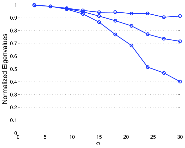
Figure 1: Plot of the eigenvalues of the OLS estimator $\hat{S}$ normalized by the eigenvalues of $S$ v.s. $\sigma$. Increasing the noise level biases the eigenvalues towards zero. A fragment of ubiquitin composed of 7 peptide planes (residue 1-8) and a specific Saupe tensor $S$ is used for the simulation and each point in the plot is computed from 200 different realizations of $\alpha_{i},\beta_{i}$’s. ]

3 Numerical results

We first demonstrate that $\hat{\sigma}$ obtained through the method described in section 2.1 is a good estimate of $\sigma$. For simulation purposes, we use a segment of ubiquitin with seven peptide planes (residue 1-8) containing 21 $N-H$, $C-CA$ and $C-N$ bonds. We note that in all the simulations, we do not consider the RDC of the nonexistent $N-H$ bond for proline. In Fig. 2(left), we plot $\hat{\sigma}$ v.s. $\sigma$. The simulation shows a close agreement between $\hat{\sigma}$ and $\sigma$, especially when the angular noise is less than 12 degrees.

We next show that the SIMEX-like method proposed in section 2 is able to reduce the bias in eigenvalue estimation, where the bias of an estimator $\hat{\theta}$ of parameter $\theta$ is defined to be

$$\text{Bias}(\hat{\theta})=\langle\hat{\theta}\rangle-\theta.$$

$\langle\cdot\rangle$ denotes averaging over the distribution of data. For this simulation, we use a specific ground truth Saupe tensor and the aforementioned ubiquitin fragment to generate precise RDC measurements. From the fragment, 200 realizations of noisy conformation are generated with $\sigma=20^{\circ}$. To obtain $\tilde{\Lambda}$, we set $n_{1}=8000$ when simulating $A_{b}$ in step (2) of the Monte Carlo procedure. In Fig. 2(right), we see that the values of $\langle\tilde{\Lambda}\rangle_{\alpha_{i},\beta_{i}}$ (Red dotted line) obtained from averaging over 200 samples are almost the same as the eigenvalues of $S$ (Black line), while there is a clear bias in the estimator $\Lambda(\hat{S})$ (Blue dotted line).

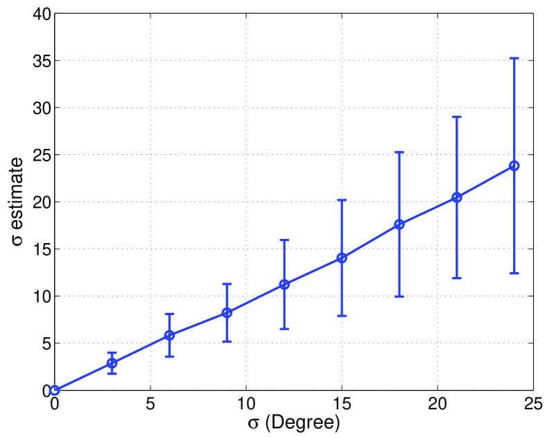
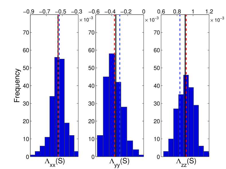
Figure 2: Above: Plot of $\hat{\sigma}$ v.s. $\sigma$. For a given noise level $\sigma$, $\hat{\sigma}$ is averaged over 200 different realizations of $\alpha_{i},\beta_{i}$’s. Below: Histograms of the diagonal entries of $\Lambda(\hat{S})$ and $\tilde{\Lambda}$ obtained from 200 fragment conformations with $20^{\circ}$ noise on the torsion angles. The values of $\Lambda(S),\langle\Lambda(\hat{S})\rangle_{\alpha_{i},\beta_{i}}$ and $\langle\tilde{\Lambda}\rangle_{\alpha_{i},\beta_{i}}$ are denoted by black, blue and red line respectively.

3.1 Estimation of Saupe tensor eigenvalues from multiple molecular fragments

While the proposed eigenvalue estimator $\tilde{\Lambda}$ has less bias, this does not obligate that $\tilde{\Lambda}$ has a lower mean squared error (MSE).This can be understood from the bias-variance decomposition, which is a classical way in statistics to decompose the MSE of an estimator $\hat{\theta}$ [28]. The MSE of an estimator $\hat{\theta}$ admits the following decomposition

$$\text{MSE}(\hat{\theta}) = \langle(\theta-\hat{\theta})^{2}\rangle$$ (30)

$$= \langle(\theta-\langle\hat{\theta}\rangle+\langle\hat{\theta}\rangle-\hat{\theta})^{2}\rangle$$ (31)

$$= \text{Bias}(\hat{\theta})^{2}+\text{Var}(\hat{\theta})+2(\theta-\langle\hat{\theta}\rangle)\langle\langle\hat{\theta}\rangle-\hat{\theta}\rangle$$ (32)

$$= \text{Bias}(\hat{\theta})^{2}+\text{Var}(\hat{\theta})$$ (33)

$\text{Var}(\hat{\theta})$ denotes the variance of $\hat{\theta}$. Although we achieve less bias with the estimator $\tilde{\Lambda}$, we pay the price of having larger variance due to bias estimation involved in obtaining $\tilde{\Lambda}$. This increase in variance can lead to $\tilde{\Lambda}$ having higher MSE than $\Lambda(\hat{S})$. From this point of view, when estimating the Saupe tensor eigenvalue using a single template fragment, the Monte Carlo method for debiasing may seem unnecessary or even disadvantageous. However, when multiple template fragments are available, the average of $\tilde{\Lambda}$ over these fragments, denoted $\tilde{\Lambda}_{\text{ave}}$, enjoys variance reduction proportional to the number of fragments. Therefore in the case when there are many fragments, it is worth paying the price of increased variance because the systematic bias error cannot be reduced via averaging. In the rest of the section, we use $\Lambda_{\text{ave}}(\hat{S})$ to denote the average of $\Lambda(\hat{S})$ over multiple fragments.

We now demonstrate the usefulness of our method under the setting of Molecular Fragment Replacement (MFR) approach [7, 12]. When RDCs are measured in two different alignment medias for a protein of unknown structure, the MFR method can construct its structure by combining short homologous fragments obtained from chemical shift and dipolar homology database mining. Typically for every protein fragment of seven residues, 10 homologous structures are searched based on the similarity of chemical shifts and the goodness of Saupe tensor fit to the observed RDC. When OLS is used to fit the Saupe tensor with design matrix $A$ constructed from homologous structures, one can average all OLS eigenvalue estimated to obtain improved estimators of the parameters such as alignment magnitude and rhombicity that depend on the eigenvalues [12]. These parameters can in turn be used in a simulated annealing procedure such as XPLOR-NIH [22] to refine the structure.

We first use synthetic data to demonstrate our method. We generate 12 random Saupe tensors, by sampling two eigenvalues from the uniform distribution on $[-10^{-3},0]$ and $[0,10^{-3}]$ respectively, and extract the third eigenvalue by requiring $\Lambda(S)_{xx}+\Lambda(S)_{yy}+\Lambda(S)_{zz}=0$. The orthogonal matrix $U(S)$ is sampled uniformly from the group of $3\times 3$ orthogonal matrices, by computing the orthogonal factor in the polar decomposition of a $3\times 3$ Gaussian random matrix [2]. After obtaining the RDC $d_{nm}$’s from the clean structure and the ground truth Saupe tensor, under each simulated alignment condition we add structural noise of magnitude $\sigma$ to every fragment of seven peptide planes of the ubiquitin structure obtained from X-ray crystallography (PDB ID 1UBQ). We only consider the first 71 residues of the 76 residues of ubiquitin, as there are few RDC reported for the last five residues of ubiquitin. This gives a total of 64 fragments. We evaluate the estimators of the Saupe tensor eigenvalues $\Lambda_{\text{ave}}(\hat{S})$ and $\tilde{\Lambda}_{\text{ave}}$ computed from the average of $\Lambda(\hat{S})$ and $\tilde{\Lambda}$ of all fragments, by comparing their fractional errors averaged over the 12 different Saupe tensors and torsion angle noise realizations in Fig. 3. The fractional error is defined as

$$\frac{\|\Lambda_{\text{ave}}(\hat{S})-\Lambda(S)\|_{F}}{\|\Lambda(S)\|_{F}}\quad\text{and}\quad\frac{\|\tilde{\Lambda}_{\text{ave}}-\Lambda(S)\|_{F}}{\|\Lambda(S)\|_{F}}.$$

In this simulation, the fractional error of $\Lambda_{\text{ave}}(\hat{S})$ is at least three times larger than $\tilde{\Lambda}_{\text{ave}}$.

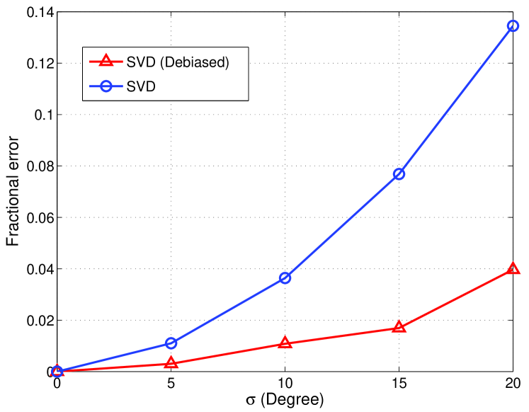
Figure 3: Plot of the fractional error of $\Lambda_{\text{ave}}(\hat{S})$ and $\tilde{\Lambda}_{\text{ave}}$ v.s. $\sigma$. Each data point is averaged over 12 different Saupe tensor and noise realizations for 1UBQ. The plot shows a clear advantage of the bias reduced estimator over the OLS estimator.

We finally apply this method to estimate the Saupe tensor of ubiquitin in two different alignment medias using the experimental RDC data in [6]. From 600 homologous structures returned by MFR homology search, each containing seven residues, we obtain 600 Saupe tensor estimates using OLS. Since we expect our method to have a significant effect for fragments severely corrupted by structural noise, we average the fragments with residual RMS above a certain threshold and plot $\Lambda_{\text{ave}}(\hat{S})$ and $\tilde{\Lambda}_{\text{ave}}$ normalized by $\Lambda(S)$ v.s. RMS thresholds. To get an estimated (and approximate) ground truth Saupe tensor $S$, we use the high resolution ubiquitin structure 1UBQ obtained from X-ray crystallography [27] to fit the RDC data. We demonstrate the results in Fig. 4. Other than the estimators for $\Lambda(S)_{yy}$ of the second alignment media which has a large percent error due to the relatively small magnitude of $\Lambda(S)_{yy}$, $\tilde{\Lambda}_{\text{ave}}$ typically achieves 0.9 of the ground truth value, whereas $\Lambda_{\text{ave}}(\hat{S})$ can shrink to 0.8 of the value of $\Lambda(S)$ when only the fragments of high RMS are used in averaging. We therefore recommend the use of our proposed bias removing method when estimating eigenvalues from multiple noisy fragments.

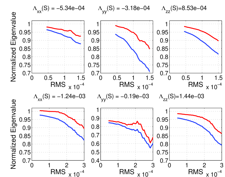
Figure 4: Plot of the eigenvalue estimators normalized by $\Lambda(S)$ v.s. residual RMS thresholds. Estimators are obtained from experimental RDC measurements in two different alignment medias. While the magnitude of $\tilde{\Lambda}_{\text{ave}}$ (Red curves) and $\Lambda_{\text{ave}}(\hat{S})$ (Blue dotted curves) both decrease as low quality (high RMS) fragments are solely used in averaging, $\tilde{\Lambda}_{\text{ave}}$ in general is within 90% of the ground truth value but $\Lambda(S)$ drops to 80% of $\Lambda_{\text{ave}}(\hat{S})$. The value of $\Lambda(S)$ for both alignment medias are indicated in the plot title.

4 Effect of additive noise on Saupe tensor estimation

So far we have been neglecting the presence of additive noise on $d_{nm}$, which is considered by [15]. We define the noisy RDC measurements corrupted by additive noise as

$$d_{\text{add}}=d+\sigma_{\text{add}}\varepsilon$$ (34)

where entries of the column vector $\varepsilon$ are i.i.d random variables with mean zero. In this section, we show using perturbation theory that this type of additive noise biases the eigenvalue magnitude positively, therefore it cannot explain the magnitude shrinkage we see when fitting the Saupe tensor to real RDC data (Fig. 4). Moreover, the order of magnitude of this positive bias is not sufficient to explain the error between $\hat{S}$ and $S$. This has been noted by the authors of [15] that in order to account for the size of the OLS misfit, an uncertainly of 2-3 Hz for the RDC measurements is required although the experimental uncertainty is only about 0.2-0.5 Hz. This is the reason why in this paper we focus on removing the bias that arises from structural noise.

Let

$$S=U(S)\Lambda(S)U(S)^{T}$$ (35)

be the eigendecomposition of $S$. Assuming the eigenvalues of $S$ are nondegenerate, the second order perturbation theory [13] states

$$\lambda_{j}(\hat{S}) \approx \lambda_{j}(S)+U(S)_{j}^{T}(\hat{S}-S)U(S)_{j}$$ (36)

$$+\sum_{\begin{subarray}{c}k=x,y,z,\\ k\neq j\end{subarray}}\frac{(U(S)_{k}^{T}(\hat{S}-S)U(S)_{j})^{2}}{\lambda_{j}(S)-\lambda_{k}(S)}.$$ (37)

Averaging the perturbation expansion over the distribution of $\varepsilon$, we get

$$\lambda_{j}(\hat{S})\approx\lambda_{j}(S)+\sum_{\begin{subarray}{c}k=x,y,z,\\ k\neq j\end{subarray}}\frac{\langle(U(S)_{k}^{T}(\hat{S}-S)U(S)_{j})^{2}\rangle_{\varepsilon}}{\lambda_{j}(S)-\lambda_{k}(S)}.$$ (38)

Here we use the fact that $\langle\hat{S}-S\rangle_{\varepsilon}=0$ since

$$\langle\hat{s}-s\rangle_{\varepsilon}=\langle(A^{T}A)^{-1}A^{T}(As+\varepsilon)-s\rangle_{\varepsilon}=\langle(A^{T}A)^{-1}A^{T}\varepsilon\rangle_{\varepsilon}=0$$

The expression in (38) reveals that in the presence of noise, the largest eigenvalue of $\hat{S}$ is always greater than the largest eigenvalue of $S$, while the smallest eigenvalue behaves in the exact opposite manner. Such effect of bias of pushing the extreme eigenvalues outwards is also commonly seen in the context of estimating the extreme eigenvalues of covariance matrices [21].

For this type of bias we now give an estimate of its order of magnitude. First we bound the numerator in the second order correction term in (38):

$$(U(S)_{k}^{T}(\hat{S}-S)U(S)_{j})^{2} = \mathrm{Tr}((\hat{S}-S)U(S)_{j}U(S)_{k}^{T})^{2}$$ (39)

$$\leq \|\hat{S}-S\|_{F}^{2}\|U(S)_{j}U(S)_{k}^{T}\|_{F}^{2}$$ (40)

$$\leq 3\|\hat{s}-s\|_{2}^{2}.$$ (41)

The first inequality results from Cauchy-Schwarz inequality, and the second inequality relies on the fact that $\|U(S)_{j}U(S)_{k}^{T}\|_{F}=1$ and $\|\hat{S}-S\|_{F}^{2}\leq 3\|\hat{s}-s\|_{2}^{2}$, which can be verified easily. It is a classical result [11] that the OLS estimator has covariance matrix

$$\langle(\hat{s}-s)(\hat{s}-s)^{T}\rangle_{\varepsilon}=\sigma_{\text{add}}^{2}(A^{T}A)^{-1},$$ (42)

therefore

$$\langle\|\hat{s}-s\|_{2}^{2}\rangle_{\varepsilon}=\sigma_{\text{add}}^{2}\mathrm{Tr}((A^{T}A)^{-1}).$$ (43)

Using (43), (39) we obtain an upperbound for the bias in (38). Taking $\lambda_{z}(\hat{S})$ for example:

$$\lambda_{z}(\hat{S})-\lambda_{z}(S)\lesssim\frac{3\mathrm{Tr}((A^{T}A)^{-1})}{\lambda_{z}(S)-\lambda_{y}(S)}\sigma_{\text{add}}^{2}$$ (44)

We now give an estimate of the order of magnitude of the bias. Since the magnitude of the extreme eigenvalues of the Saupe tensor is around $10^{-3}$, for example for the two RDC datasets acquired for ubiquitin, we simply assume $\lambda_{z}(S)-\lambda_{y}(S)\sim 10^{-4}$. The typical experimental uncertainty for RDC measurements is about 0.2 Hz - 0.5 Hz, and the dipolar coupling constant $D_{nm}^{\text{max}}$ for e.g. $N-H$ bonds, is about 23 kHz, therefore the noise magnitude $\sigma_{\text{add}}$ of the additive noise on the normalized dipolar coupling is about $0.5/(23\times 10^{3})\approx two\times 10^{-5}$. For ubiquitin, the average value of $\mathrm{Tr}((A^{T}A)^{-1})$ for fragments containing seven peptide planes is about 1.35. Using these numbers in (44), we get

$$\lambda_{z}(\hat{S})-\lambda_{z}(S)\lesssim 1.6\times 10^{-5},$$

which amounts to 1-2% error when $\lambda_{z}(S)\sim 10^{-3}$. This cannot explain the 10% or larger error in fitting Saupe tensor to real RDC datasets using homology fragments in the previous section.

We present a simulation to illustrate the bias in OLS eigenvalues estimation in the presence of additive noise. We use the Saupe tensor eigenvalues for ubiquitin in the first alignment media presented in Fig. 4, and a ubiquitin fragment consisting of seven peptide planes (residue 1-8) for this simulation. We generate noisy datasets using the noise model

$$d_{\text{add}}=As+\sigma_{\text{add}}\varepsilon.$$

For every noise level, we average $\Lambda(\hat{S})$ normalized by $\Lambda(S)$ over 500 different realizations of $s$ and $\varepsilon$ where entries of $\varepsilon$ are i.i.d. random normal variables. The different realization of $s$ are generated from $S=U(S)\Lambda(S)U(S)^{T}$ where $\Lambda(S)$ is fixed but $U(S)$ is sampled uniformly from the orthogonal group in $\mathbb{R}^{3}$. We vary the orientation of the Saupe tensor since it is clear from (38) that the bias depends on $U(S)$. We change $\sigma_{\text{add}}$ from 0 to 10% of $\lambda_{z}(S)$ and present the results in Fig. 5. We note again from previous calculations, $\sigma_{\text{add}}\sim 2\times 10^{-5}$, which amounts to 2-3% of the $\lambda_{z}(S)=0.85\times 10^{-3}$ considered. As shown in the simulation and our crude estimate, such magnitude of noise gives rise to bias error of about 1%. Even in the case of having very noisy RDC (having noise magnitude 10% of $\lambda_{z}(S)$), the bias error caused by additive noise is around 3%. Whereas in a typical MFR search with torsion angle tolerance being set to $\pm 20^{\circ}-30^{\circ}$ [30], the simulation in Fig. 1 suggests structural noise can cause bias error sometimes much greater than 10%. Therefore in this paper we focus on removing the bias that arises from structural noise. In the case when accurate template structure is available and the additive noise is a concern, we refer readers to the appendix for the removal of such bias using an analytic expression derived from perturbation theory.

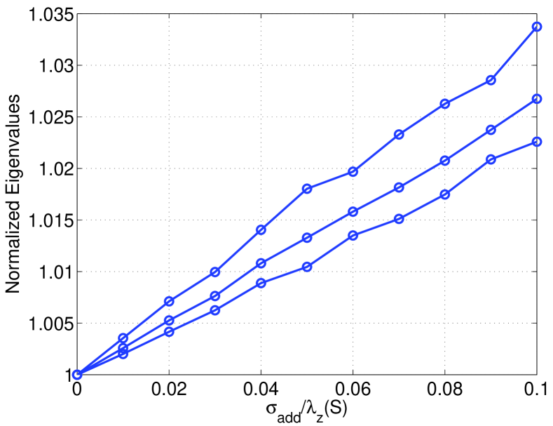
Figure 5: Plot of the three eigenvalues of the OLS estimator $\hat{S}$ normalized by the eigenvalues of $S$ v.s. $\sigma_{\text{add}}$ under noise model (34). Each point is averaged over 2000 noise and Saupe tensor realizations. Increasing the noise level biases the eigenvalues positively, unlike the case for structural noise. At 10% noise level, the bias is about 3%.

5 Conclusion

We observe a negative bias when estimating the Saupe tensor eigenvalues through the classical SVD method, in the presence of structural noise on the template structure due to torsion angle noise. We present a Monte Carlo method that simulates noise on the template structure by perturbing the torsion angles and use the simulated structure to estimate the bias in the eigenvalues. We demonstrate the effectiveness of our method in reducing the error arising from bias when estimating Saupe tensor eigenvalues from multiple protein fragments, which is a natural setting to consider when building protein structure from homologous substructures.

6 Acknowledgement

The research of AS was partially supported by award R01GM090200 from the NIGMS, by awards FA9550-12-1-0317 and FA9550-13-1-0076 from AFOSR, by award LTR DTD 06-05-2012 from the Simons Foundation, and the Moore Foundation Data Driven Discovery Investigator award.

7 Appendix

7.1 Removing bias from additive noise

Define a linear operator $L:\mathbb{R}^{5}\rightarrow\mathbb{R}^{3\times 3}$ that forms a Saupe tensor $S$ from the vector $s$ as

$$L(s)=\begin{bmatrix}-s(1)-s(2)&s(3)&s(4)\\ s(3)&s(1)&s(5)\\ s(4)&s(5)&s(2)\end{bmatrix},\quad s\in\mathbb{R}^{5}.$$ (45)

For the additive noise model (34) we have

$$\hat{S}=L(\hat{s})=L((A^{T}A)^{-1}A^{T}d_{\text{add}})=S+L((A^{T}A)^{-1}A^{T}\varepsilon).$$ (46)

We also define the adjoint operator of $L$, $L^{*}:\mathbb{R}^{3\times 3}\rightarrow\mathbb{R}^{5}$ through the relation

$$\mathrm{Tr}(X^{T}L(y))=L^{*}(X)^{T}y,$$ (47)

for every $y\in\mathbb{R}^{5}$ and $X\in\mathbb{R}^{3\times 3}$. To obtain the form of $L^{*}$, we let $y\in\{e_{1},\ldots,e_{5}\}$, where $e_{i}(i)=1$ and $e_{i}(j)=0$ if $j\neq i$. Plugging such $y$ into Eq. (47), we get

$${L^{*}(X)}_{1} = -X_{xx}+X_{yy}$$ (48)

$${L^{*}(X)}_{2} = -X_{xx}+X_{zz}$$ (49)

$${L^{*}(X)}_{3} = X_{xy}+X_{yx}$$ (50)

$${L^{*}(X)}_{4} = X_{xz}+X_{zx}$$ (51)

$${L^{*}(X)}_{5} = X_{yz}+X_{zy}$$ (52)

Using such notion of the adjoint operator, the perturbation series in (38) can be written as

$$\langle\lambda_{j}(\hat{S})\rangle_{\varepsilon}\approx\lambda_{j}(S)+\sum_{\begin{subarray}{c}k=x,y,z,\\ k\neq j\end{subarray}}\frac{\langle((\hat{s}-s)^{T}L^{*}(U(S)_{k}U(S)_{j}^{T}))^{2}\rangle_{\varepsilon}}{\lambda_{j}(S)-\lambda_{k}(S)}\\ =\lambda_{j}(S)+\mathrm{Tr}\bigg{[}\bigg{(}\sum_{\begin{subarray}{c}k=x,y,z,\\ k\neq j\end{subarray}}\frac{L^{*}(U(S)_{k}U(S)_{j}^{T})L^{*}(U(S)_{k}U(S)_{j}^{T})^{T}}{\lambda_{j}(S)-\lambda_{k}(S)}\bigg{)}\text{Var}(\hat{s})\bigg{]}$$ (53)

where

$$\text{Var}(\hat{s})\equiv\langle(\hat{s}-s)(\hat{s}-s)^{T}\rangle_{\varepsilon}=(A^{T}A)^{-1}\sigma_{\text{add}}^{2}.$$ (54)

Therefore we can subtract the second order term in (53) to correct for the bias in the eigenvalues. Although we do not know the eigenvectors and eigenvalues of $S$, we can replace them with the eigenvectors and eigenvalues $\hat{S}$. This change will only affect on the higher order terms in the perturbation series.

References

- [1] Martin Blackledge, Recent progress in the study of biomolecular structure and dynamics in solution from residual dipolar couplings, Progress in Nuclear Magnetic Resonance Spectroscopy 46 (2005), no. 1, 23–61.
- [2] Gordon Blower, Random matrices: high dimensional phenomena, vol. 367, Cambridge University Press, 2009.
- [3] Raymond J Carroll, David Ruppert, Leonard A Stefanski, and Ciprian M Crainiceanu, Measurement error in nonlinear models: a modern perspective, CRC press, 2006.
- [4] G Clore, A Gronenborn, and A Bax, A robust method for determining the magnitude of the fully asymmetric alignment tensor of oriented macromolecules in the absence of structural information, Journal of magnetic resonance 133 (1998), no. 1, 216–21.
- [5] John R Cook and Leonard A Stefanski, Simulation-extrapolation estimation in parametric measurement error models, Journal of the American Statistical Association 89 (1994), no. 428, 1314–1328.
- [6] Gabriel Cornilescu, John L Marquardt, Marcel Ottiger, and Ad Bax, Validation of protein structure from anisotropic carbonyl chemical shifts in a dilute liquid crystalline phase, Journal of the American Chemical Society 120 (1998), no. 27, 6836–6837.
- [7] Frank Delaglio, Georg Kontaxis, and Ad Bax, Protein structure determination using molecular fragment replacement and NMR dipolar couplings, Journal of the American Chemical Society 122 (2000), no. 9, 2142–2143.
- [8] Bradley Efron and Robert J Tibshirani, An introduction to the bootstrap, CRC press, 1994.
- [9] Theo Gasser, HG Muller, and Volker Mammitzsch, Kernels for nonparametric curve estimation, Journal of the Royal Statistical Society. Series B (Methodological) (1985), 238–252.
- [10] Michael Grant and Stephen Boyd, CVX: Matlab software for disciplined convex programming, version 2.1, http://cvxr.com/cvx, March 2014.
- [11] Jürgen Groß, Linear regression, vol. 175, Springer Science & Business Media, 2003.
- [12] Georg Kontaxis, Frank Delaglio, and Ad Bax, Molecular fragment replacement approach to protein structure determination by chemical shift and dipolar homology database mining, Methods in Enzymology 394 (2005), 42–78.
- [13] Lev Davidovich Landau and Evgenii Mikhailovich Lifshitz, Quantum mechanics: non-relativistic theory, vol. 3, Elsevier, 2013.
- [14] Rebecca S Lipsitz and Nico Tjandra, Residual dipolar couplings in NMR structure analysis, Annu. Rev. Biophys. Biomol. Struct. 33 (2004), 387–413.
- [15] Judit A Losonczi, Michael Andrec, Mark WF Fischer, and James H Prestegard, Order matrix analysis of residual dipolar couplings using singular value decomposition, Journal of Magnetic Resonance 138 (1999), no. 2, 334–342.
- [16] Jens Meiler, Jeanine J Prompers, Wolfgang Peti, Christian Griesinger, and Rafael Brüschweiler, Model-free approach to the dynamic interpretation of residual dipolar couplings in globular proteins, Journal of the American Chemical Society 123 (2001), no. 25, 6098–6107.
- [17] Eva Meirovitch, Donghan Lee, Korvin FA Walter, and Christian Griesinger, Standard tensorial analysis of local ordering in proteins from residual dipolar couplings, The Journal of Physical Chemistry B 116 (2012), no. 21, 6106–6117.
- [18] T Michael Sabo, Colin A Smith, David Ban, Adam Mazur, Donghan Lee, and Christian Griesinger, Orium: Optimized rdc-based iterative and unified model-free analysis, Journal of biomolecular NMR 58 (2014), no. 4, 287–301.
- [19] L. Salmon and M. Blackledge, Investigating protein conformational energy landscapes and atomic resolution dynamics from NMR dipolar couplings: a review, Rep Prog Phys 78 (2015), no. 12, 126601.
- [20] AZ. Saupe, Kernresonanzen in kristallinen flüssigkeiten und in kristallinflüssigen lösungen. teil i, Naturforsch. 19 (1964), no. a, 161–171.
- [21] Juliane Schäfer and Korbinian Strimmer, A shrinkage approach to large-scale covariance matrix estimation and implications for functional genomics, Statistical applications in genetics and molecular biology 4 (2005), no. 1.
- [22] Charles D Schwieters, John J Kuszewski, Nico Tjandra, and G Marius Clore, The Xplor-NIH NMR molecular structure determination package, Journal of Magnetic Resonance 160 (2003), no. 1, 65–73.
- [23] LA Stefanski and JR Cook, Simulation-extrapolation: the measurement error jackknife, Journal of the American Statistical Association 90 (1995), no. 432, 1247–1256.
- [24] Joel R Tolman, A novel approach to the retrieval of structural and dynamic information from residual dipolar couplings using several oriented media in biomolecular nmr spectroscopy, Journal of the American Chemical Society 124 (2002), no. 40, 12020–12030.
- [25] Joel R Tolman and Ke Ruan, NMR residual dipolar couplings as probes of biomolecular dynamics, Chemical Reviews 106 (2006), no. 5, 1720–1736.
- [26] John W Tukey, Exploratory data analysis, Addison-Wesley Series in Behavioral Science: Quantitative Methods, Reading, Mass.: Addison-Wesley, 1977, vol. 1, 1977.
- [27] Senadhi Vijay-Kumar, Charles E Bugg, and William J Cook, Structure of ubiquitin refined at 1.8Å resolution, Journal of Molecular Biology 194 (1987), no. 3, 531–544.
- [28] Larry Wasserman, All of statistics: a concise course in statistical inference, Springer Science & Business Media, 2013.
- [29] Lukas N Wirz and Jane R Allison, Fitting alignment tensor components to experimental RDCs, CSAs and RQCs, Journal of Biomolecular NMR (2015), 1–5.
- [30] Zhengrong Wu, Frank Delaglio, Keith Wyatt, Graeme Wistow, and Ad Bax, Solution structure of s-crystallin by molecular fragment replacement NMR, Protein science 14 (2005), no. 12, 3101–3114.
- [31] Markus Zweckstetter and Ad Bax, Evaluation of uncertainty in alignment tensors obtained from dipolar couplings, Journal of Biomolecular NMR 23 (2002), no. 2, 127–137.