Strong Gravity Approach to QCD and General Relativity

Abstract

A systematic study of a Weyl type of action, which is scale free and quadratic in the curvature, is undertaken. The dynamical breaking of this scale invariance induces general relativity (GR) as an effective long distance limit of the theory. We prove that the corresponding field equations of the theory possess an effective pure Yang-Mills (i.e. QCD without quarks) potential, which describes the asymptotic freedom and color confinement properties of QCD. This inevitably leads to the solutions of quantum Yang-Mills existence on R⁴ (with its characteristic mass gap), and dark matter problems. The inherent Bern-Carrasco-Johansson (BCJ) double-copy and gauge-gravity duality properties of this formulation lead to the solutions of the neutrino mass and dark energy problems. This approach provides a strong gravity basis for the unification of quantum Yang-Mills theory (QYMT) with Einstein GR.

Keywords: Weyl action, BCJ double-copy, gauge-gravity duality.

I Introduction

”Who of us would not be glad to lift the veil behind which the future lies hidden; to cast a glance at the next advances of our science and at the secrets of its developments during future centuries?” $-$ David Hilbert (1900).

”It is by the solution of problems that the investigator tests the temper of his steel; he finds new methods and new outlooks, and gains a wider and freer horizon” $-$ David Hilbert (1900).

In the early seventies Abdus Salam and his co-workers proposed the concept of strong gravity, in which the successive self -interaction of a nonlinear spin-2 field was used to describe a non-abelian field of strong interactions. This idea was formulated in a two-tensor theory of strong and gravitational interactions, where the strong tensor fields are governed by Einstein-type field equations with a strong gravitational constant $G_{f}\approx 10^{38}$ times the Newtonian constant $G_{N}$. Within the framework of this proposal, tensor fields were identified to play a fundamental role in the strong-interaction physics of quantum chromodynamics (QCD) CJI ; ASJ ; CSI ; DJS ; YNE ; ASCS .

All the calculations done in the numerical lattice QCD and other related experiments indicate that QCD, the worthy theory of strong interactions, possesses gauge symmetry based on the group $SU(3)-$color of quantum Yang-Mills theory (QYMT). Gravitational interactions also have similar symmetry (the coordinate invariance in a space-time manifold), but resist quantization. This prevents physicists from constructing a quantum theory of gravity based on the gauge principle, and also inhibits the direct unification of gravity with strong interaction IANC .

The origin of the difficulties is now clear to us: QCD action is scale invariantly quadratic in the field strengths $F_{\mu\nu}^{i}$ (i.e.non-unitary) and renormalizable, while the Einstein-Hilbert action for pure gravity is unitary and nonrenormalizable. Thus, the unification of gravity with QCD seems unattainable; however, that is not the case: The valiant attempt to disprove this prima facie impossibility offers an outstanding example of the inspiring effect which such a very special and apparently important solution may have upon physics community.

Having now recalled to mind the origin of the problem, let us turn to the question of whether there is an existing unification scheme that can be used to solve the problem. Strong gravity formulation is such the unification scheme that allows the gravity to be merged with QYMT. In this case, a gravitational action which possesses quadratic terms in the curvature tensor has been shown to be renormalizable (KSS , P.963 & P.967). Here, the resulting non-gauge-invariant divergences are absorbed by nonlinear renormalizations of the gravitational fields and Becchi-Rouet-Stora transformations (KSS , P.953). In the following, the dynamical breaking of the scale invariance of Weyl action (which describes the short distance behavior of strong gravity theory) induces: (1) perturbative/short-range component of  the non-relativistic QCD potential, and non-relativistic quantum electrodynamic (QED) potential. (2) Einstein general relativity as an effective long distance limit of the theory $-$ This is the fons et origo of the gauge/gravity duality; and the solution to the quantum Yang-Mills existence on R⁴ and dark matter problems, within the strong gravity formulation.

The catch here is that quantum gravity (i.e. a quantum mechanically induced gravity) cannot be derived straightforwardly by quantizing nonrenormalizable Einstein GR but Weyl action which leads to Einstein’s theory of gravity at large distancesIANC ; in the same way the gauge theory of Glashow-Weinberg-Salam, $G_{EW}=SU(2)_{L}\times U(1)_{Y},$ reduces to $U(1)_{Q}$ after the spontaneous symmetry breakdownEW ; JCA .

QCD possesses four remarkable properties that strong gravity must have for it to be called a complete theory of strong interactions. The   first is asymptotic freedom (i.e., the logarithmic decrease of the QCD coupling constant $\alpha_{s}(Q_{0}^{2})\sim 1/(\ln$ $Q_{0}^{2})$ at large momentum transfers, or equivalently the decrease of $\alpha_{s}$ at small distances, $\alpha_{s}(r)\sim 1/(\ln r)$) which permits one to perform consistent theoretical computations of hard processes using perturbation theory. This property also implies an increase of the running coupling constant at small momentum transfer, that is, at large distances. The second important property is the confinement, in which quarks and gluons are confined within the domain of their strong interaction and hence cannot be observed as real physical objects. The physical objects observed experimentally, at large distances, are hadrons (mesons and baryons). The third characteristic property is the dynamical breakdown of chiral symmetry, wherein the vector gauge theories with massless Dirac fermion fields $\psi$ are perfectly chiral symmetric. However, this symmetry is broken dynamically when the vector gauge theory is subjected to chiral $SU(2)$ rotations. This is the primary reason why chiral symmetry is not realized in the spectrum of hadrons and their low energy interactionsBIF ; QHN . The fourth property is the mass gap($\Delta$). Here, every excitation of the QCD vacuum has minimum positive energy (i.e. $\Delta>0$); in other words, there are no massless particles in the theoryEW ; JCA . Additionally,

strong gravity must also be able to reproduce the two fundamental parameters of QCD (i.e., coupling $\alpha_{s}$ and fundamental quark mass $m_{q}$ JBER , P.178).

Thus, the three demands that must be met by strong gravity theory for it to be called a unification scheme for QYMT-GR are:

(1) It must admit the four QCD properties afore-listed.

(2) It must be able recover the fundamental parameters of QCD (i.e., $\alpha_{s}$ and $m_{q}$).

(3) It must be able to reproduce Einstein’s general relativity as the limiting case of its long-distance behavior.

Any theory that fulfills these three demands can be termed ”a unified theory of nature”.

In the present paper, we study the structure of a dynamically broken scale-invariant quantum theory (Weyl’s action) within the context of strong gravity formulation, and its general properties. The major problem which has to be faced immediately is the unresolved question of unitarity of pure gravity: Weyl’s action is non-unitary while the Einstein-Hilbert action for pure gravity is unitary. This problem is circumvented within the framework of strong gravity: where the unitary Einstein-Hilbert term is induced after the breakdown of the scale invariance of Weyl’s action (ASCS , P.324). To put it in a proper and succinct context, Einstein GR emerges from the Weyl’s action after the dynamical breakdown of its scale invariance. Hence Einstein’s theory of gravity is not a fundamental theory of nature but the classical output of the more fundamental  gluon-dependent Weyl’s action.

The paper is organized as follows. In section II, we briefly review the BCJ double-copy construction of gravity scattering amplitudes. Section III is devoted to the review of strong gravity theory. Most importantly, we prove that BCJ double-copy construction exists within the strong gravity formulation. The calculation of the dimensionless strong coupling constant is done in the section IV. The theoretically obtained value is tested experimentally in the section V. We present strong gravity as a massive spin-two theory in the section VI. Here, we show that the dynamics of strong gravity theory is fully symmetric, but its vacuum state is asymmetric. We also show in this section that electroweak and custodial symmetries can be induced dynamically. Critical temperature, fundamental mass and mass gap of the QCD vacuum are obtained in the section VII. This leads to the derivation of the effective pure Yang-Mills potential. The gauge-gravity duality property of strong gravity theory is studied in the section VIII. We also show that strong gravity possesses UV regularity and dynamical chiral symmetry breaking in this same section.  Confinement and asymptotic freedom properties of the strong gravity is studied in the section IX. In this section, we calculate the energy density of QCD vacuum. The existence of quantum Yang-Mills theory on $R^{4}$ is established in the section X. The vacuum stabilizing property of Higgs boson with mass $m_{H}=129GeV$ is studied in section XI. The solutions to the neutrino mass, dark energy and dark matter problems are presented in the sections XII, XIII and XIV respectively. The physics of the repulsive gravity and cosmic inflation is presented in the section XV. Conclusion is given in the section XVI.

II Theoretical Preliminaries

Research in strong gravity has always had a rather unique flavor, due to conceptual difficulty of the field, and remoteness from experiment. We argue, in this paper, that if the conceptual misconception $-$ namely, that gravity is bedeviled with many untamable infinities $-$ that beclouds the field could be circumvented, then the complexity enshrined in the field would become highly trivialize.

The most powerful tool for removing this conceptual difficulty is encoded in a long-known formalism: that the asymptotic states of gravity can be obtained as tensor products of two gauge theory states (i.e. $gravity=gauge\otimes gauge$). This idea was extended to certain interacting theories, in 1986, by Kawai, Lewellen and Tye TOGO1 ; and to strong-gravitational theory by A. Salam and C. Sivaram in 1992 ASCS . The modern understanding of this double-copy formalism is largely due to the work of Bern, Carrasco and Johansson (BCJ). Formally, double-copy construction (also known as BCJ construction) is used to construct a gravitational scattering amplitude by using modern unitarity method, and the scattering amplitudes of two gauge theory as building blocks TOGO2 ; TOGO3 . This pathbreaking technique of computing perturbative scattering amplitudes, which led to a deeper understanding of quantum field theory, gravity, and to powerful new tools for calculating QCD processes, was awarded the 2014 J.J. Sakurai Prize for Theoretical Particle Physics TOGO4 .

BCJ construction has overturned the long-accepted dogma on Einstein’s GR, which posits that GR is nonrenormalizable. This new approach breaths new life into the search for a fundamental unified theory of nature based on the ”supergravity” approach. Supergravity tries to tame the infinities encountered in the Einstein’s theory of gravity by adding ”supersymmetries” to it. In a variant of the theory called $N=8$ supergravity, which has eight new ”mirror-image” particles (gravitinos) allow physicists to tame the infinities present in the Einstein’s theory of gravity: other variants of supergravity are $N=2,4$ Yang-Mills-Einstein-Supergravity (YMESG) and $N=0$ Yang-Mills-Einstein (YME) theories (TOGO5 ; TOGO6 , and the references therein) $-$ Supergravity is like a ”young twig, which thrives and bears fruit only when it is grafted carefully and in accordance with strict horticultural rules upon the old stem”.

As to the $N=0$ YME theory (where $N=0$ means that there are no supersymmetries in the theory), we claim that this theory is by no means different from the broken-scale-invariant Weyl’s action. This assertion can only be true if this action naturally possesses BCJ and guage-gravity duality properties. The BCJ property is established in the next subsection, and we show that the potential, carried by the broken-scale-invariant Weyl’s action, possesses this property in the subsection D of section III of this paper. The gauge-gravity duality property of strong gravity is established in section VIII: this is our ”guide post on the mazy paths to the hidden truths” of neutrino mass and dark energy problems. The discovery made here is that both problems are connected by the effective vacuum energy (or effective Weyl Lagrangian).

II.1 Perturbative Quantum Gravity and Color/ Kinematics Duality: A Review

QCD (one of the variants of Yang-Mills theory) is the current well-established theory of the strong interactions. Due to its asymptotic-free nature, perturbation theory is usually applied at short distances; and the ensuing predictions have achieved an astonishing success in explaining a wide range of phenomena in the domain of large momentum transfers. Upon closer consideration the question arises: Can perturbation theory be used to explore the quantum behavior of gravity at short distances as well? The answer to that question is a resounding yes! The discovery of BCJ principle is now our window into the quantum world of gravity with tamable infinities at short distances. This principle states that, regardless of the number of spacetime dimensions and loops, a valid gravity scattering amplitude is obtained by replacing color factors with kinematic numerators in a gauge-theory scattering amplitude. The resulting gauge-coupling doubling is called BCJ/double-copy property TOGO2 ; TOGO3 .

The gluon’s scattering amplitudes, (in terms of cubic graphs) at L loops and in D dimensions, are given by (TOGO2 ; TOGO3 ; TOGO5 ; TOGO6 , and the references therein):

$$A_{m}^{(L)}=i^{L-1}g_{\alpha}^{m-2+2L}\underset{i\text{ }\in\text{ }cubic}{\sum}\int\frac{d^{LD}\ell}{(2\pi)^{LD}}\frac{1}{S_{i}}\frac{c_{i}n_{i}}{D_{i}}$$ (1)

where $m$ is the number of points, $g_{\alpha}$ is the dimensionless gauge coupling, $S_{i}$ are the standard symmetry factors and $D_{i}$ are denominators encoding the structure of propagator in the cubic graphs. $c_{i}$ are the color factors and $n_{i}$ are the kinematic numerators. BCJ construction posits that within the gauge freedom of individual cubic graphs, there exist unique amplitude representations that make kinematic factors $n_{i}$ obey the same general algebraic identities as color factors. Hence, color/kinematics duality holds: $n_{i}\iff c_{i}$ TOGO2 ; TOGO3 .

The double-copy principle then states that once the color/kinematics duality is satisfied (i.e., $n_{i}\iff c_{i}$), the L-loop scattering amplitudes of a supergravity theory (with $N\geq 4$) are given by

$$M_{m}^{(L)}=i^{L-1}\left(\frac{k_{\alpha}}{2}\right)^{m-2+2L}\underset{i\text{ }\in\text{ }cubic}{\sum}\int\frac{d^{LD}\ell}{(2\pi)^{LD}}\frac{1}{S_{i}}\frac{n_{i}^{2}}{D_{i}}$$ (2)

where dimensionless $k_{\alpha}$ is the gravity coupling; and it is assumed that the two involved gauge fields are from the same Yang-Mills theory. From Eqs. (1) and (2), we have

$$A_{m}^{(L)}=M_{m}^{(L)}\iff k_{\alpha}=2g_{\alpha}$$ (3)

Eq.(3), which is valid for all variants of supergravity with $N\geq 4$, is the expected gauge-coupling doubling or BCJ property. This property shows that gravitons and gluons should be part of a fundamental unified theory of nature.

However, the devil is in the detail: the color-kinematics duality ($n_{i}\iff c_{i}$) is more or less a conjecture; and the scattering-amplitude method of probing the quantum nature of gravity is full of many mathematical landmines. Nevertheless, the conclusions of N = 8 supergravity theory are indisputable. For we are convinced that the gauge-coupling doubling and gauge-gravity duality should exist in the correct theory of quantum gravity without appealing to supersymmetries. This is where strong gravity theory (or point-like gravity) kicks in. Our present knowledge of the theory of strong gravity puts us in a position to attack successfully the problem of quantum gravity/point-like gravity by using powerful-mathematical tools (formula operators from differential geometry with their duality and supersymmetry-like properties) bequeathed to us by antiquity.

We conclude this section with a great quote from one of the greatest revolutionary mathematicians the world has ever known (David Hilbert) TOGO7 : ”If we do not succeed in solving a mathematical problem, the reason frequently consists in our failure to recognize the more general standpoint from which the problem before us appears only as a single link in a chain of related problems. After finding this standpoint, not only is this problem frequently more accessible to our investigation, but at the same time we come into possession of a method which is applicable also to related problems” $-$The ”standpoint” discovered in this paper is the strong gravity theory.

III Strong Gravity Theory: A Review

We briefly review the standard formulation of strong gravity theory in this section: (for more details see CJI ; ASJ ; CSI ; DJS ; YNE ; ASCS ; KSS and the references therein). Beginning with the two-gluon phenomenological fields (i.e. double-copy construction), we re-establish strong gravity as a renormalizable four-dimensional quantum gauge field theory by varying Weyl action with respect to the spacetime metric constructed out of the two-gluon configuration. In this case, the two-point configuration (which leads to the quantization of space-time itself) naturally introduces a minimum length $2r_{g}$ (i.e. ”intergluonic distance”); where $r_{g}$ is the ”gluonic radius”. It should be emphasized here that this way of quantizing space-time begins from the trajectories of two 2-gluons,i.e., curves or paths of the geometry used. This method of constructing spacetime geometry from 2-gluon phenomenology has been shown to be compatible with nature: The visualization of the QCD vacuum (i.e.visualization of action density of the Euclidean-space QCD vacuum in three-dimensional slices of a $24^{3}\times 36$ spacetime lattice), by D. B. Leinweber, has shown that empty space is not empty; rather it contains quantum fluctuations in the gluon field at all scales (this is famously referred to as ”gluon activity in a vacuum”) TOGO8 . This can only mean one thing: that gluon field is the fundamental field of nature, and the spacetime metric/gravity is emergent from 2-gluon configuration. This is the main argument of BCJ/double-copy construction. Simpliciter!

By taking the vacuum states of hadron to be colorless (i.e. color-singlet), the approximation of an external QCD potential (the hadron spectrum above these levels) can be generated by color-singlet quanta. Based on the fully relativistic QCD theory, these contributions have to come from the summations of suitable Feynman diagrams in which dressed n-gluon configurations are exchanged between several ”flavors” of massless quarks. Thus, the simplest such system (with contributions from n-gluon irreducible parts $n=2,3,...,\infty$ and with the same Lorentz quantum numbers) will have the quantum numbers of 2-gluon. The color singlet external field is then constructed from QCD gluon field as a sum (DJS , P.572):

$$G_{\mu}^{a}G_{\nu}^{b}\eta_{ab}+G_{\mu}^{a}G_{\nu}^{b}G_{\sigma}^{c}d_{abc}+...$$ (4)

where $\eta_{ab}$ is the $SU(3)_{C}$ color-metric, $d_{abc}$ is the totally symmetric $8\otimes 8\otimes 8\rightarrow 1$ coefficient and $G_{\mu}^{a}$ is the dressed gluon field. The curvature would be generated by the derivatives of $G_{\mu}^{a}$ (ASCS ,P.323). The 2-gluon configuration can then be written from Eq.(4) as

$$g_{\mu\nu}(x)=G_{\mu}^{a}G_{\nu}^{b}\eta_{ab}$$ (5)

with

$$g=\det(g_{\mu\nu}(x))$$ (6)

Eq.(5) is taken as the dominating configuration in the excitation systematics. In this picture, the metric is constructed from a gluon-gluon interaction, and the gluon-gluon effective gravity-like potential (effective Riemannian metric, $g_{\mu\nu}$) would act as a metric field passively gauging the effective diffeomorphisms (general coordinate transformations), just as is done by the Einstein metric field for the general coordinate transformations of the covariance group (YNE , P.174).

It is crystal-clear that Eq.(5), as put forward by the proponents of strong gravity, is by no means different from the double-copy structure of gauge fields in the BCJ construction ($gravity=gauge\otimes gauge$); as such we should be able to arrive at the same conclusions. The BCJ formalism (double-copy construction) is formulated by using scattering-amplitude method. Similarly, we show that double-copy construction can be obtained by using formula operators from the differential geometry. Our approach puts BCJ formalism on a proper mathematical footing: it puts flesh on the bones of BCJ formalism.

III.1 Scale-Invariant-Confining Action for Strong Gravity Theory

In analogy with the scale-invariant QCD action which is quadratic in the field strengths $F_{\mu\nu}^{i}$(with dimensionless coupling), we have the corresponding Weyl action for gravity (ASCS , P.322):

$$I_{W}=-\alpha_{s}\int d^{4}x\sqrt{-g}C_{\alpha\beta\gamma\delta}C^{\alpha\beta\gamma\delta}$$ (7)

where $\alpha_{s}$ is purely dimensionless and can be made into a running coupling constant $\alpha_{s}(Q_{0}^{2}).$ It’s worth noting that Eq.(7) is not only generally covariant but also locally scale invariant (IANC , P.6). The Weyl’s tensor ($C_{\alpha\beta\gamma\delta})$ is constructed out of the corresponding Riemann curvature tensor, i.e., the covariant derivatives involving gauge fields, characterized with the generators of the conformal group. In the following, the metric is generated by Eq.(5) (ASCS , P.323).

The Weyl curvature tensor is defined as the traceless part of the Riemann curvature TT :

$$C_{\alpha\beta\gamma\delta} =R_{\alpha\beta\gamma\delta}-\frac{1}{n-2}(R_{\alpha\gamma}\eta_{\beta\delta}-R_{\alpha\delta}\eta_{\beta\gamma}$$

$$-R_{\beta\gamma}\eta_{\alpha\delta}+R_{\beta\delta}\eta_{\alpha\gamma})$$

$$+\frac{1}{(n-1)(n-2)}R(\eta_{\alpha\gamma}\eta_{\beta\delta}-\eta_{\alpha\delta}\eta_{\beta\gamma})$$ (8)

Eq.(8) is constructed by using the trace-free property of Weyl tensor:

$$\eta^{\alpha\gamma}C_{\alpha\beta\gamma\delta}=C_{\beta\alpha\delta}^{\alpha}=0$$ (9)

By contracting Eq.(8) with itself, we get

$$C_{\alpha\beta\gamma\delta}C^{\alpha\beta\gamma\delta} =R_{\alpha\beta\gamma\delta}R^{\alpha\beta\gamma\delta}-\frac{4}{(n-2)}R_{\beta\delta}R^{\beta\delta}$$

$$+\frac{2}{(n-2)(n-1)}R^{2}$$ (10)

In  four-dimension ($n=4$), Eq.(10) reduces to;

$$C^{2}\equiv C_{\alpha\beta\gamma\delta}C^{\alpha\beta\gamma\delta}=R_{\alpha\beta\gamma\delta}R^{\alpha\beta\gamma\delta}-2R_{\beta\delta}R^{\beta\delta}+\frac{1}{3}R^{2}$$ (11)

Thus, Eq.(7) becomes,

$$I_{W}=-\alpha_{s}\int d^{4}x\sqrt{-g}(R_{\alpha\beta\gamma\delta}R^{\alpha\beta\gamma\delta}-2R_{\beta\delta}R^{\beta\delta}+\frac{1}{3}R^{2})$$ (12)

III.2 Gauss-Bonnet Invariant Theorem

For space-time manifold topologically equivalent to flat space, the Gauss-Bonnet theorem relates the various quadratic terms in the curvature as IANC :

$$I_{GB}=-\alpha_{s}\int d^{4}x\sqrt{-g}(R_{\alpha\beta\gamma\delta}R^{\alpha\beta\gamma\delta}-4R_{\alpha\beta}R^{\alpha\beta}+R^{2})=0$$ (13)

Using this property, we can rewrite Eq.(12) as

$$I_{W}\longrightarrow I_{WGB}=I_{W}-I_{GB}=I_{W}$$ (14)

$$I_{W}=-2\alpha_{s}\int d^{4}x\sqrt{-g}\left[R_{\beta\delta}R^{\beta\delta}-\frac{1}{3}(R_{\gamma}^{\gamma})^{2}\right]$$ (15)

where $R_{\beta\delta}$ is the Ricci tensor, which is a symmetric tensor due to the Bianchi identities of the first kind, and its trace defines the scalar curvature $R_{\gamma}^{\gamma}=R$ (SW-2 , P.153). By using Eqs.(7) and (15), we have

$$\int d^{4}x\sqrt{-g}\left(R_{\beta\delta}R^{\beta\delta}-\frac{1}{3}R^{2}\right)=\frac{1}{2}\int d^{4}x\sqrt{-g}C_{\alpha\beta\gamma\delta}C^{\alpha\beta\gamma\delta}$$ (16)

Eq.(15) leads to the field equations TOGO9 :

$$\sqrt{-g}g_{\mu\alpha}g_{\nu\beta}\frac{\delta I_{W}}{\delta g_{\alpha\beta}}=-\frac{1}{2}T_{\mu\nu}$$ (17)

Eq.(17) would be of fourth-order in the form (ASCS , P.323):

$$\frac{1}{2}g_{\mu\nu}(R_{\gamma}^{\gamma})_{;\delta}^{;\delta}+R_{\mu\nu}{}_{;\delta}^{;\delta}-R_{\mu;\nu;\delta}^{\delta}-R_{\nu;\mu;\delta}^{\delta}-2R_{\mu\delta}R_{\nu}^{\delta}+\frac{1}{2}g_{\mu\nu}R_{\gamma\delta}R^{\gamma\delta}$$

$$-\frac{1}{3}[2g_{\mu\nu}(R_{\gamma}^{\gamma})_{;\delta}^{;\delta}-2(R_{\gamma}^{\gamma})_{;\mu;\nu}-2R_{\gamma}^{\gamma}R_{\mu\nu}+\frac{1}{2}g_{\mu\nu}(R_{\gamma}^{\gamma})^{2}]$$

$$=\frac{1}{4\alpha_{s}}T_{\mu\nu}$$ (18)

The corresponding fourth-order Poisson equation and its linearized solution are given as(ASCS , P.323 & 325):

$$\delta_{s}\nabla^{4}V =km_{0}\delta^{3}(r)$$

$$V(r) =\alpha r$$ (19)

It is clear from Eq.(18) that its left-hand side vanishes whenever $R_{\mu\nu}$ is zero (the vanishing of a tensor is an invariant statement (SW-2 ,P.146)), so that any vacuum solution of Einstein equations would also satisfy the ones from the quadratic action. A complete exact solution of the field Eq.(18) (with metric signature $+---$) for a general spherical symmetric vacuum metric is given as (ASCS , P.323-324):

$$ds^{2}=\alpha dt^{2}-\beta dr^{2}-r^{2}d\theta^{2}-r^{2}\sin^{2}\theta d\phi^{2}$$ (20)

where

$$\alpha=1-\frac{\lambda_{1}}{r}-\lambda_{2}r-\lambda_{3}r^{2}$$ (21)

$$\beta=\left[\alpha\right]^{-1}$$ (22)

$\lambda_{1},$ $\lambda_{2},$ and $\lambda_{3}$ in Eq.(21) are suitable constants, related to the coupling constant. Dimensional analysis and natural unit formalism then tell us that coupling constant ($\alpha)$ would remain dimensionless provided that $\lambda_{1}$ carries the dimension of distance ([L]$GeV^{-1}$), $\lambda_{2}$ the dimension of mass ([M]$GeV$), and $\lambda_{3}$ the dimension of squared mass ([M]${}^{2},$ $GeV^{2}$). If we take the mass to be the mass of the quark ($m_{q}$), then we can rewrite Eq.(21) as

$$\alpha_{s}=1-\frac{\lambda_{1}}{r}-m_{q}r-m_{q}^{2}r^{2}$$ (23)

For the pure Yang-Mills theory (i.e. QCD without quarks), $m_{q}\rightarrow 0$ and Eq.(23) reduces to

$$\alpha_{s}=1-\frac{\lambda_{1}}{r}$$ (24)

Based on the strong gravity theory and the formalism of the vacuum solution of Einstein field equations CSI ; SW-2 ; CWKJ , $\lambda_{1}=G_{f}$ $m$.

With this value, Eq.(24) reduces to

$$\alpha_{s}=g_{00}=1-\frac{G_{f}\text{ }m}{r}$$ (25)

and Eq.(20) becomes

$$ds^{2} =\left(1-\frac{G_{f}\text{ }m}{r}\right)dt^{2}-\left(1-\frac{G_{f}\text{ }m}{r}\right)^{-1}dr^{2}$$

$$-r^{2}d\theta^{2}-r^{2}\sin^{2}\theta d\phi^{2}$$ (26)

where mass $m$ is the only allowed mass in the theory, and is due to the self-interaction of the two gluons (glueball). Eq.(26) is the well celebrated Schwarzschild vacuum metric except that instead of normal Newtonian gravitational constant ($G_{N}\approx 10^{-19}GeV^{-1}$), we have strong-gravitational constant ($G_{f}\approx 1GeV^{-1}$).

III.3 Broken Scale Invariance and Perturbative/Short Distance Behavior

Once we have $\Lambda_{QCD}\equiv G_{f}^{-1}\approx 1GeV$, the scale invariance would be broken. An additional Einstein-Hilbert term linear in the curvature would be induced, but the full action would still preserve its general coordinate invariance (ASCS ,P.324):

$$I_{eff}=-\int d^{4}x\sqrt{-g}\left(\alpha_{1}R_{\mu\nu}R^{\mu\nu}-\alpha_{2}R^{2}+k^{-2}\alpha_{3}R\right)$$ (27)

Here the induced Einstein-Hilbert term incorporates the phenomenological term $1/k^{2}=\frac{1}{32\pi G_{N}}$ (KSS , P.954 & 967): this term is called graviton propagator/ ”pure Yang-Mills” propagator . By comparing Eq.(27) with Eq.(15), we have

$$\alpha_{1} =\alpha_{3}=2$$

$$\alpha_{2} =\frac{2}{3}$$ (28)

Using natural units formalism, we can write

$$k^{-2}=\frac{1}{32\pi G_{N}}\approx 1\times 10^{17}GeV$$ (29)

where $G_{N}\approx 10^{-19}GeV^{-1}$ (in natural units) (ASJ , P. 2668).

Eq.(27) gives rise to the mixture of fourth-order and second-order field equations(ASCS , P.324), whose solutions for the field of a localized mass involves Yukawa and the normal $1/r$ potential terms.

$$\alpha\nabla^{4}V+\beta\nabla^{2}V\approx km_{0}\delta^{3}(r)$$ (30)

The corresponding solution of the Eq.(30) for a point mass source is given as (VDS , P. 3):

$$V(r)=\frac{C_{1}}{r}-\frac{C_{2}}{r}e^{-\beta_{1}/r}+\frac{C_{3}}{r}e^{-\beta_{2}/r}$$ (31)

where $C_{1}=k^{2}M/8\pi\alpha_{3},$ $C_{2}=k^{2}M/6\pi\alpha_{3},$ $C_{3}=k^{2}M/42\pi\alpha_{3,\text{ }}\beta_{1}=\left[\alpha_{3}^{1/2}(\alpha_{1}k^{2})^{-1/2}\right]\times G_{f}^{3/2},$ and $\beta_{2}=\alpha_{3}^{1/2}\left[2\left(3\alpha_{2}-\alpha_{1}\right)k^{2}\right]^{-1/2}\times G_{f}^{3/2}.$ $M$ is unknown invariant mass (but we identified it to be the invariant mass of the final hadronic state of the theory, $M\equiv m$ (because final observable particle state must be color singlet)).

By using Eqs.(28) and (29), $\beta_{2}=\infty$ and thus Eq.(31) reduces to

$$V(r)=\frac{C_{1}}{r}-\frac{C_{2}}{r}e^{-\beta_{1}/r}$$ (32)

$$C_{1} =\frac{k^{2}m}{16\pi}$$

$$C_{2} =\frac{k^{2}m}{12\pi}$$

$$\beta_{1} =k^{-1}G_{f}^{3/2}$$ (33)

As expected, the resulting infinity $\beta_{2}=\infty$ is tamed by the nonlinear nature of the Weyl’s action.

From Eqs.(32) and (33), we have

$$V(r)=\frac{k^{2}\text{ }m}{16\pi r}\left(1-\frac{4}{3}e^{-\beta_{1}/r}\right)$$ (34)

Eq.(32) is the exact equation obtained for the broken scale invariance and perturbative behavior of strong gravity in (ASCS , P.325).

III.4 Double-copy Construction in Strong Gravity

From Eq.(34), we can write

$$V(r)=\frac{k_{\alpha}^{2}\text{ }}{16\pi r}C$$ (35)

where the dimensionless gravity coupling $k_{\alpha}^{2}\equiv k^{2}$ $m=32\pi G_{N}\times m$ and $C\equiv 1-\frac{4}{3}e^{-\beta_{1}/r}$ is the ”group-theoretic constant” of strong gravity theory.

It is to be recalled that the interaction energy, to the leading order, of two static (i.e., symmetric) color sources of QCD without quarks (pure Yang-Mills theory) is given by TOGO10 ; TOGO11 ; TOGO12 ; TOGO13 :

$$E(r)=\frac{g_{\alpha}^{2}\text{ }}{4\pi r}C$$ (36)

Where dimensionless gauge coupling $g_{\alpha}^{2}\equiv g^{2}(r)\times m_{rg}$, and $m_{rg}$ is an arbitrary renormalization group scale formally invoked, in quantum field theory, to keep the scale-dependent gauge coupling ($g^{2}(r)$) dimensionless. Since Eq.(35) is also the energy of two interacting gluons, we can write (from Eqs.(35) and (36))

$$V(r)=E(r)\iff k_{\alpha}=2g_{\alpha}$$ (37)

Eq.(37) is the required BCJ property. We have therefore proved the existence of double-copy construction in strong gravity. It is remarkable to note that despite different approaches taken by supergravity (scattering amplitude method) and strong gravity (effective potential method), we still arrive at the same conclusion (see Eqs. (3) and (37)).

IV QCD Evolution

The body of experimental data describing the strong interaction between nucleons (which is the non-perturbative aspect of QCD for $r\longrightarrow\infty$) is consistent with a strong coupling constant behaving as $\alpha_{s}\approx 1$ TOGO14 : obviously this aspect of QCD is consistent with the Eq.(25) for $r\longrightarrow\infty.$

One of the discoveries about strong force is that it diminishes inside the nucleons, which leads to the free movement of gluons and quarks within the hadrons. The implication for the strong coupling is that it drops off at very small distances. This phenomenon is called ”asymptotic freedom” or perturbative aspect of QCD, because gluons and massless quarks approach a state where they can move without resistance in the tiny volume of the hadron TOGO15 . Hence for the strong gravity to describe the perturbative aspect of QCD correctly, it must reproduce the value of strong coupling constant $\alpha_{s}$ (by using the observed properties of gluons: the mediators of strong force) that is compatible with the experimental data. This is what we set out to do in this section.

IV.1 Gluon Density

The first thing to note here is that gluon, being a bosonic particle, obeys Bose-Einstein statistics. The Fermi-Dirac and Bose-Einstein distribution functions are given as (PCR , P. 115);

$$\aleph_{r}=\frac{g_{r}}{e^{\sigma_{1}+\sigma_{2}\in_{r}}\pm 1}$$ (38)

where the positive sign applies to fermions and the negative to bosons. $\aleph_{r}$ is the number of particles in the single-particle states, $g_{r}$ is the degenerate parameter, $\sigma_{1}$ is the coefficient of expansion of a gas of weakly coupled particles (an ideal configuration for describing the asymptotic freedom/perturbative regime of QCD) inside the volume $V$. $\sigma_{2}$ is the Lagrange undetermined multiplier and $\in_{r}$ is energy of the $r$-$th$ state. The value of $"\sigma_{1}"$ for boson gas at a given temperature is determined by the normalization condition (PCR , P. 112 and 115);

$$N=\underset{r}{{\displaystyle\sum}}\frac{g_{r}}{e^{\sigma_{1}+\sigma_{2}\in_{r}}-1}$$ (39)

The summation sign in Eq.(39) can be converted into an integral, because for a particle in a box, the states of the system have been found to be very close. Using the density of single-particle states function, Eq.(39) reduces to;

$$N=\underset{0}{\overset{\infty}{\int}}\frac{D(\in)d\in}{e^{\sigma_{1}+\sigma_{2}\in}-1}$$ (40)

where $D(\in)d\in$ is the number of allowed states in the energy range $\in$ to $\in+d\in$ and $\in$ is the energy of the single-particle state. Using the density of states as a function of energy, we have (PCR , P. 290);

$$D(\in)d\in\text{ }=\frac{4\pi V}{h^{3}}2m\in\left(\frac{m}{p}\right)d\in$$

with

$$p=\sqrt{2m\in}$$

$$D(\in)d\in\text{ }=2\pi V\left(\frac{2m}{h^{2}}\right)^{3/2}\in^{1/2}d\in$$ (41)

where $p$ is the momentum of particle, $m$ its mass and $h$ is the Planck constant. By putting Eq.(41) into Eq.(40), we have

$$N=2\pi V\left(\frac{2m}{h^{2}}\right)^{3/2}\underset{0}{\overset{\infty}{\int}}\frac{\in^{1/2}d\in}{e^{\sigma_{1}+\sigma_{2}\in}-1}$$ (42)

but $\sigma_{1}=\sigma_{2}\times\mu_{eff}$ and $\sigma_{2}=1/kT.$ $\mu_{eff}$ is the effective potential, $k$ is the Boltzmann constant and $T$ denotes temperature (PCR , P.116). Since there is no restriction on the total number of bosons (gluons), the effective potential is always equals to zero ($\mu_{eff}=0$) (this is true for the case where the minimum of the effective potential continuously goes to zero as temperature growsCSB ). Thus, Eq.(42) reduces to;

$$N=2\pi V\left(\frac{2m}{h^{2}}\right)^{3/2}\underset{0}{\overset{\infty}{\int}}\frac{\in^{1/2}d\in}{e^{\in/kT}-1}$$ (43)

By using the standard integral(where $\varsigma(z)$ is the Riemann zeta function and $\Gamma(z)$ is the gamma function)

$$\underset{0}{\overset{\infty}{\int}}\frac{x^{z-1}dx}{e^{x}-1}=\varsigma(z)\Gamma(z)$$ (44)

Eq.(43) becomes

$$N=2.61V\left(\frac{2\pi mkT}{h^{2}}\right)^{3/2}$$ (45)

Using $m=E/c^{2}$ and the average kinetic energy of boson gas in three-dimensional space $E=3kT/2,$ Eq. (45) reduces to;

$$\frac{N}{V}=\left[\frac{(2.61)(3\pi)^{3/2}k^{3}}{(hc)^{3}}\right]T^{3}$$ (46)

Define $n_{g}\equiv\frac{N}{V}$ and $\Xi\equiv\left[\frac{(2.61)(3\pi)^{3/2}k^{3}}{(hc)^{3}}\right]=2.522\times 10^{7}(mK)^{-3}.$ Hence the gluon density ($n_{g}$) can be expressed as;

$$n_{g}=\Xi T^{3}$$ (47)

Eq.(47) is the required result for the finite temperature and density relation for gluon.

IV.2 Strong-gravity Coupling Constant

The principle of general covariance tells us that the energy-momentum tensor in the vacuum (with zero matter and radiation) must take the form;

$$T_{00}=K\langle\rho\rangle$$ (48)

Here $\langle\rho\rangle$ has the dimension of energy density and $K$ describes a real (strong-) gravitational field SER . Hence Eq.(48) reduces to;

$$T_{00}=K(E_{vac})^{4}$$ (49)

and $K=g_{00}=C_{QCD}\times C_{grav}(strong-gravity$ coupling). $C_{QCD}$ is a dimensionless coefficient which is entirely of QCD origin and is related to the definition of QCD on a specific finite compact manifold. Similarly, $C_{grav}$ is a dimensionless coefficient which is entirely of gravitational origin SER ; LZW ; FRU ; SWEN . Therefore Eq.(49) becomes

$$T_{00}=g_{00}(E_{vac})^{4}$$ (50)

Recall that energy density ($\rho_{vac}$) can also be written as

$$\rho_{vac}=\frac{E_{vac}}{V}=V^{-1}\times E_{vac}$$ (51)

Eq.(51) is justified by the standard box-quantization procedure SER . Hence we have

$$\rho_{vac}=n_{g}\times E_{vac}$$ (52)

where $n_{g}\equiv V^{-1}$ (number density).

From the average kinetic energy for gas in three-dimensional space, we have $T=2E_{vac}/3k.$ With this value, Eq.(47) reduces to

$$n_{g}=\frac{8\Xi(E_{vac})^{3}}{27k^{3}}$$ (53)

Thus Eq.(52) becomes

$$\rho_{vac}=\frac{8\Xi(E_{vac})^{4}}{27k^{3}}$$ (54)

Eq.(54) is the energy density of a single gluon. But based on double-copy construction (see section II, Eqs.(3) and Eq.(37)), Eq.(54) is multiplied by 2, and thus,

$$2\rho_{vac}=\frac{16\Xi(\Delta\varepsilon_{vac})^{4}}{27k^{3}}$$ (55)

Eq.(55) now represents two-point correlator-vacuum energy density. By comparing Eq.(50) with Eq.(55), we have

$$\alpha_{s}=g_{00}=\frac{16\Xi}{27k^{3}}=2.336\times 10^{19}(meV)^{-3}$$

As $1m=5.070\times 10^{15}GeV^{-1}$, the above equation leads to

$$\alpha_{s}=g_{00}=C_{QCD}\times C_{grav.}=0.1797$$ (56)

Eq.(56) is the required strong (-gravity) coupling constant at the starting point of QCD evolution. In the next section, we show the compatibility of Eq.(56) with the perturbative QCD, which is the theory that describes asymptotic freedom regime analytically.

V Perturbative Quantum Chromodynamics

Computations in perturbative QCD are formally based on three conditions: (1) that hadronic interactions become weak at small invariant separation $r\ll\Lambda_{QCD}^{-1}$; (2) that the perturbative expansion in $\alpha_{s}(Q_{0}^{2})$ is well-defined mathematically; (3) factorization dictates that all effects of collinear singularities, confinement, non-perturbative interactions, and the dynamics of bound state can be separated constituently at large momentum transfer in terms of (process independent) structure functions $G_{i/H}(x,Q),$ hadronization functions $D_{H/i}(z,Q),$ or in the case of exclusive processes, distribution amplitudes $\phi_{H}(x_{i},Q)$ AHM ; GPL . The asymptotic freedom property of perturbative QCD($\beta_{0}=11-(2/3)n_{f}$) is given as (ASO , P. 1):

$$\alpha_{s}(Q_{0}^{2})=\frac{4\pi}{\beta_{0}\ln(\frac{Q_{0}^{2}}{\Lambda^{2}})}<0.2\text{ \ for }Q_{0}^{2}>20GeV^{2}$$ (57)

In the framework of perturbative QCD, computations of observables are expressed in terms of the renormalized coupling $\alpha_{s}(\mu_{R}^{2})$. When one takes $\mu_{R}$ close to the scale of the momentum transfer $Q_{0}$ in a given process, then $\alpha_{s}(\mu_{R}^{2}\sim Q_{0}^{2})$ is indicative of the effective strength of the strong interaction in that process. Eq.(57) satisfies the following renormalization group equation (RGE) GDISS :

$$\mu_{R}^{2}\frac{d\alpha_{s}}{d\mu_{R}^{2}}=\beta(\alpha_{s})=-(b_{0}\alpha_{s}^{2}+b_{1}\alpha_{s}^{3}+b_{2}\alpha_{s}^{4}+O(\alpha_{s}^{5}))$$ (58)

with

$$b_{0}=(33-2n_{f})/12\pi$$ (59)

$$b_{1}=(153-19n_{f})/24\pi^{2}$$ (60)

$$b_{2}=(2857-\frac{5033}{9}n_{f}+\frac{325}{27}n_{f}^{2})/128\pi^{3}$$ (61)

where Eqs.(59-61) are referred to as the 1-loop, 2-loop and 3-loop beta-function coefficients respectively. The minus sign in Eq.(58) is the origin of asymptotic freedom, i.e., the fact that the strong coupling becomes weak for hard processes. Eq.(58) shows that RGE is dependent on the correct value of a purely dimensionless strong coupling constant ( $\alpha_{s}$). Thus the precise calculation of its value (without appealing to the choice of renormalization scheme and scale choice $Q_{0}^{2}$) would be the holy grail of perturbative QCD.

V.1 Experimental Test

We begin by reviewing the systematic study of QCD coupling constant from deep inelastic measurements in (VGKA and the references therein), where many experimental data were collected and analyzed at the next-to-leading order of perturbative QCD (see Tables 2,3 and 6 of VGKA ) by using deep inelastic scattering ($DIS$) structure functions $F_{2}(x,Q^{2}).$In these experimental results, we are more interested in the $\alpha_{s}(90GeV^{2})=0.1797$ (in the Table 6 of VGKA ) obtained when the number of points is 613. This is the exact value we obtained theoretically in Eq.(56). Hence, we have not only demonstrated that the perturbative expansion for hard scattering amplitudes converges perturbatively at $\alpha_{s}=\alpha_{s}(90GeV^{2})=0.1797$ but also able to prove that QCD is a strong-gravity-derived theory: an astonishing discovery! We have also validated the asymptotic freedom property of perturbative QCD given in Eq.(57): namely, that the starting point of QCD evolution is $Q_{0}^{2}=90GeV^{2}$ for $\alpha_{s}=0.1797<0.2.$

Having tested Eq.(56) experimentally, we therefore proceed to rewrite the renormalization group equation (Eq.(58) ) as:

$$\beta(\alpha_{s})=-\left[b_{0}(0.1797)^{2}+b_{1}(0.1797)^{3}+b_{2}(0.1797)^{4}+...\right]$$ (62)

Eq.(62) is an echo of  ”composition independence or universality property” of the coupling $\alpha_{s}$ to all orders in the perturbative expansion for hard scattering amplitudes.

VI Strong Gravity as a Massive Spin-two Theory

In the Einstein’s GR, the Schwarzschild vacuum is the solution to the Einstein field equations that describes the gravitational field generated by a spherically symmetric mass $m$, on the assumption that the electric charge, and orbital angular momentum ($L$) of the mass are all zero CWKJ .

It turns out that the Schwarzschild vacuum solution of the Einstein field equations can be understood in terms of the Pauli-Fierz relativistic wave equations for massive spin-2 particles which would mediate a short-range tensor force (CSI , P. 117). It follows that the two interacting gluon fields ($G_{\mu}^{a}$ and $G_{\nu}^{b})$ are considered to be dressed gluon fields of the gravitational field, i.e., the colors of the gluon fields are covered or hidden within the spacetime base-manifold ($\eta_{ab}$) of the color $-$ $SU(3)$ principal bundle (DJS , P. 572), thereby making the observable asymptotic states of gravity to be color-singlet/color-neutral. Hence the resulting glueball (massive particle formed as a result of the self-interaction of two gluons) of the theory (with spherically symmetric mass $m$ and quantum numbers $J^{PC}=2^{-+}$) would still have the total angular momentum of $2$. The validity of this statement is proved by using the well-known Pauli-Fierz relativistic wave equations for massive particles of spin-2(CSI , P. 124):

$$\square\phi_{\mu\nu}+m^{2}\phi_{\mu\nu}=0$$ (63)

$$\partial_{\mu}\phi^{\mu\nu}=0\text{ (coordinate gauge condition)}$$ (64)

$$\phi_{\mu}^{\mu}=0\text{ (conformal gauge condition)}$$ (65)

$$\phi_{\mu\nu}=\phi_{\nu\mu}\text{ (symmetric condition)}$$ (66)

For the symmetric condition (Eq.(66)), the coordinate gauge condition given in Eq.(64) eliminates four out of the ten components of the wave function $\phi_{\mu\nu}$ of the Eq.(63); and the condition given in Eq.(65) eliminates one more, leaving 5 degrees of freedom:

$$2S+1=D=5\Longrightarrow S=2$$ (67)

As a result of the Eq.(67), the following is true: strong gravity, as a massive spin-2 theory, has five degrees of freedom ($D=5$).

Recall that the parity (P) and charge (C) quantum numbers can be expressed by

$$P=(-1)^{J+1}$$ (68)

$$C=(-1)^{J}$$ (69)

and

$$J=L+S$$ (70)

where $J$ is the total angular momentum, $L$ is the orbital angular momentum and $S$ is the spin.

Thus, for the Schwarzschild vacuum solution (i.e., $L=0$), we have

$$J^{PC}=2^{-+}$$ (71)

Requiring instead that $\phi_{\mu\nu}\neq\phi_{\nu\mu}$ (antisymmetric condition), we would have obtained $2S+1=D=1\Longrightarrow S=0$ and $J^{PC}=0^{-+}$, which is a pseudoscalar state. An important consequence of this discovery is that the underlying dynamics of the strong gravity theory is fully symmetric (i.e. $\phi_{\mu\nu}=\phi_{\nu\mu}\Longrightarrow S=2$ ) but its ground/vacuum state is asymmetric (i.e. $\phi_{\mu\nu}\neq\phi_{\nu\mu}\Longrightarrow S=0;$ meaning that the vacuum state must have massive spin-zero particle(s) $-$ glueball/meson with mass $m$): this is a formal description of spontaneous symmetry-breaking phenomenon.

VI.1 Effective Lagrangian of a Massive Spin-2 Theory

By using effective field theory (EFT) and the property of strong gravity (as a massive spin-2 theory, $D=5$), the effective Lagrangian of the theory is characterized by TOGO16 :

$$L=\underset{i}{\sum}\frac{O_{i}}{M_{X}^{d_{i}-4}}$$ (72)

where $O_{i}$ are operators constructed from the light fields (with light mass), and information on any heavy degrees of freedom ( with heavy mass M_X) is encoded in the coupling $\frac{1}{M_{X}^{d_{i}-4}}$. For $i=1$, we have

$$L=\frac{O_{1}}{M_{X}^{d_{1}-4}}$$ (73)

Using $D=d_{1}=5$ means that the operator $O_{1}$ must carry the dimension of squared energy ($O_{1}\sim E^{2}$) for the effective Lagrangian to carry the dimension of energy:

$$L=\frac{E^{2}}{M_{X}}$$ (74)

Eq.(74) is the effective Lagrangian of the strong gravity theory. The invariant mass/energy operator $E^{2}=p_{\mu}p^{\mu}=m^{2}$ is called a flat space/Poincarė invariant. This is characterized by an irreducible representation of the Poincarė group (with spin $J$ ), and can be used to describe a composite field (CSI , P. 133-137) with five intrinsic degrees of freedom (i.e. $D=d_{1}=5$). The importance of this statement will be made manifest in the next subsection.

VI.2 Groups of Motions in Strong Gravity Admitting Custodial and Electroweak Symmetries

The fundamental theorem in the theory of strong gravity (as a massive spin-2 theory) contains two statements, namely:

(1) Strong gravity is a pseudo-gravity (YNE , P.173).

(2) Strong gravity, as a massive spin-2 field theory, has five degrees of freedom. The first statement means that the strong gravity must have a fundamental group $SO(n_{1},n_{2})$. The group $SO(n_{1},n_{2})$ is the special real pseudo-orthogonal group in $n_{1}+n_{2}$ dimensions. This group has a non-compact group that is isomorphic to a generalized rotation group (involving spherical (with positive curvature) and hyperbolic (with negative curvature) rotations) in $R^{n_{1},n_{2}}$. Its maximal compact subgroup is given as $SO(n_{1})\times SO(n_{2}).$The second statement forces us to write $n_{1}+n_{2}=5$.

From the Eq.(5), the dressed gluon field $G_{\mu}^{a}$ can be separated into asymptotic-flat connection ($N_{\mu}^{a}$), i.e. the constant curvature (zero-mode) of the field and the normal gluon field ($A_{\mu}^{a}$): $G_{\mu}^{a}=N_{\mu}^{a}+A_{\mu}^{a}$ (DJS , P.572 & YNE , P.174). By using the de Sitter group formalism for the spacetime of constant curvature, the non-compact groups (de Sitter groups) for strong gravity are $SO(4,1)$ and $SO(3,2)$. The group $SO(4,1)$ is associated with the spacetime manifold of constant positive curvature (denoted by $S(+)$), representing spherical rotations, and $SO(3,2)$ is associated with the manifold of constant negative curvature (denoted by $S(-)$), representing hyperbolic rotations. The two spaces are embedded in the manifold with signature ($+--$). The maximal compact subgroups for the two non-compact groups are (CSI , P. 132):

$$SO(4)\times SO(1)\approx SO(4)\approx SU(2)\times SU(2)$$ (75)

$$SO(3)\times SO(2)\approx SU(2)\times U(1)$$ (76)

Eqs.(75) and (76) can be used to label left-right and isospin-hypercharge symmetries respectively:

$$SU(2)_{L}\times SU(2)_{R}$$ (77)

$$SU(2)_{L}\times U(1)_{Y}$$ (78)

Eq.(77) is called custodial symmetry of the Higgs sector. This symmetry is spontaneously broken to the diagonal/vector subgroup after the Higgs doublet acquires a nonzero vacuum expectation value (VEV): $SU(2)_{L}\times SU(2)_{R}\longrightarrow SU(2)_{V}$ TOGO17 . Eq.(78) is the electroweak gauge symmetry of the Standard Model (SM) of particle physics.

To break the electroweak symmetry at the weak scale and give mass to quarks and leptons, Higgs doublets (that can sit in either $5_{H}$ or $\overline{5}_{H})$ are needed. The extra 3 states are color triplet Higgs scalars. The couplings of these color triplets violate lepton and baryon number, and also allows the decay of nucleons through the exchange of a single color triplet Higgs scalar. In order not to violently disagree with the non-observation of nucleon (e.g. proton) decay, the mass of the single color triplet must be greater than $\sim 10^{11}GeV$ TOGO18 . It is to be remarked here that this heavy mass would not disallow the violation of lepton and baryon number: this is the key to unlocking the mystery of neutrino mass problem. We shall return to this a little later.

If the composite light field (with its five independent components) in the subsection A of section VI is taken to be the Higgs field, transforming in five-dimensional representation (i.e. $5_{H}$), then nature would be permanently cured of its vacuum catastrophe disease. In this case the invariant mass/energy operator of the light field would now be taken to be the VEV of the Higgs doublets (i.e. $E\equiv\upsilon=246GeV$), and the heavy mass of color triplet Higgs scalar would be encoded in the coupling $1/M_{X}^{d_{1}-4}=1/M_{X}$. Here $M_{X}$ is the heavy mass characteristic of the symmetry-breaking scale of the high-energy unified theory TOGO19 . Once the high-energy unified theory that is compatible with nature is found, the value of $M_{X}$ will show up automatically. This is where pure Yang-Mills propagator kicks in.

VI.3 Type-A 331 Model

One of the beyond-SM’s of particle physics is the $SU(3)_{C}\times SU(3)_{L}\times U(1)_{X}$  or $331$ model, in which the three fundamental interactions (i.e. electromagnetic, weak and strong interactions) of nature are unified at a particular energy scale $M_{U}$. This model is formulated by extending the electroweak sector of the SM gauge symmetry. The unification of the three interactions occurs at the energy scale $M_{U}\approx 1\times 10^{17}GeV$ in the type-A variant of this model. In this variant of the model, the 331 symmetry is broken to reproduce the SM electroweak sector at the energy scale of $M_{X}=1.63\times 10^{16}GeV$ TOGO20 . It is apparent from the Eq.(29) that $k^{-2}=M_{U}=1\times 10^{17}GeV-$ this is not surprising because electromagnetic, strong and weak nuclear interactions are all variants of Yang-Mills interaction $-$ Hence the type-A 331 model is compatible with the nature and $M_{X}$ (which is identified as the mass of the single color triplet Higgs scalar) $=1.63\times 10^{16}GeV$. Thus Eq.(74) becomes

$$L=\frac{E^{2}}{M_{X}}=\frac{\left(246GeV\right)^{2}}{1.63\times 10^{16}GeV}=3.7\times 10^{-3}eV$$ (79)

and the symmetry-breaking pattern is

$$SU(3)_{L}\times U(1)_{X}\overset{M_{X}}{\longrightarrow}SU(2)_{L}\times U(1)_{Y}\overset{E^{2}}{\longrightarrow}U(1)_{Q}$$ (80)

It is to be emphasized that the calculated value in the Eq.(79) is purely based on the principle of naturalness: a composite field with five independent components, which occurs naturally out of the strong gravity formulation, is identified as the Higgs field $H$ transforming in five-dimensional representations ($5_{H}$).   As we shall soon show, Eq.(79) connects the solution of the dark energy problem to the neutrino mass problem.

The chain of symmetry-breakings in the Eq.(80) has varying energy scales but the Lagrangian $L$ of the whole system remains invariant: the physics of vacuum seems to obey effective field theory rather than quantum field theory.

VII Some Consequences of Strong Gravity and their Physical Interpretations

This section is entirely devoted to the consequences of strong gravity. In this case, we show the hitherto unknown connection between hadronic size, physical lattice size and gluonic radius ($r_{g}$). From this, we calculate the second-order phase transition/critical temperature $T_{c},$ and the fundamental hadron mass of QCD.

VII.1 Calculation of the Gluonic Radius and Second-order Phase Transition Temperature

The configuration  at $T>T_{c}$ for mass of the glueball for pure $SU(3)_{C}$ is shown in the Fig.1 TOGO21 . Where $2r_{g}$ is the intergluonic invariant separation.$\ S$ and $P$ represent scalar and pseudoscalar glueball / gauge fields respectively. This figure is a perfect representation of  2-gluon phenomenological field. It is interesting to note that Fig.1 has exactly the same structure with one-loop graviton self-energy diagram (KSS , P. 955). This is not a mere coincidence, it only shows the compatibility of Eq.(5) with the tetrad formulation of GR, and the existence of double-copy construction in all the variants of quantum gravity theory. In what follows, we will heavily rely on the correctness of the Fig.1 as the valid geometry for strong gravity theory from the point of view of 2-gluon phenomenology (double-copy construction).

We can therefore rewrite Eq.(25) for $T_{c}$ and gluonic radius $r_{g}$ as

$$T_{c}=\frac{\left[1-\alpha_{s}\right]r_{g}}{G_{f}}$$ (81)

 By using Eq.(56), Eq.(81) becomes

$$T_{c}=\frac{0.8203r_{g}}{G_{f}}$$ (82)

We now calculate the value of $r_{g}$ by using the value of the momentum transfer, at which $\alpha_{s}$ converges perturbatively (i.e., $Q_{0}^{2}=90GeV^{2}$): see subsection A of section V.

Recall that the energy-wavelength relation is given as

$$Q_{0}=\frac{hc}{\lambda}$$ (83)

Based on the geometry of Fig.1, we can write its associated wavelength as;

$$\lambda=2\pi r_{g}$$ (84)

Hence Eq.(83) reduces to;

$$Q_{0}=\frac{hc}{2\pi r_{g}}$$

$$r_{g}=\frac{\hslash c}{Q_{0}}$$ (85)

But $Q_{0}^{2}=90GeV^{2}\Longrightarrow$ $Q_{0}=9.487GeV$ and $\hslash$ $=6.582\times 10^{-16}eVs.$ Thus Eq.(85) reduces to,

$$r_{g}=2.08\times 10^{-17}m$$ (86)

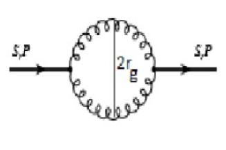
Figure 1: Diagram for the contribution to the glueball (two-gluon) mass.

Eq.(86) is the required gluonic radius. Clearly Eq.(86) is related to the radius of hadron ($r_{h}$) CJI ; ASCS ; CSI ; DJS ; YNE :

$$r_{h}=10\times r_{g}$$ (87)

From the lattice QCD simulation performed at the initial run $\beta=2.2$ on a $L^{3}T=24^{3}\times 48$ lattice gives the physical lattice size ($L_{a}$) of $2.08\times 10^{-15}m$ AAKS . By using Eq.(86), we can write

$$L_{a}=10^{2}\times r_{g}$$ (88)

Hence Eqs.(86-88) show the connection between the gluonic radius, radius of hadron and the physical lattice size.

It is generally believed that at sufficiently high temperature / density, the QCD vacuum undergoes a phase transition into a chirally symmetric phase. Here, the chirally symmetric phase transition will be second-order phase transition $iff$ the conditions $T_{c}\neq 0$ and $\mu_{eff}=0$ hold simultaneously CSB . Interestingly, we have a priori claimed, during the calculation of gluon density, that $\mu_{eff}=0$: an assertion that is justified by the fact glueball, a self-conjugated particle with neutral color and zero electric charge, has a vanishing effective/chemical potential (i.e. $\mu_{eff}=0$) (TOGO19 , P.565). Thus the second-order chiral phase transition temperature is calculated by using gluonic radius (Eq.(86)) , and thus Eq.(82) becomes

$$T_{c}=0.129GeV=129MeV$$ (89)

where $G_{f}=10^{38}\times G_{N}=6.674\times 10^{27}m^{3}kg^{-1}s^{-2}$ and $1GeV=1.78\times 10^{-27}kg.$

Hence, the chiral second-order phase transition in the strong gravity theory occurs when $T_{c}=129MeV$ and $\mu_{eff}=0.$ Exactly the same values were obtained in CSB ; DSE for second-order chiral phase transition in QCD vacuum. We have thus established that strong gravity theory exhibits second-order chiral symmetry in the limit of vanishing quark masses ( $m_{q}\rightarrow 0$). It is worth noting here that the pure $SU(3)_{C}$ vacuum metric (Eq.(26)), obtained in the limit $m_{q}\rightarrow 0$, is compatible with the glueball mass configuration given in the Fig.1, because Fig.1 was obtained in the limit of vanishing quark masses TOGO21 .

VII.2 Charmed Final Hadronic State of Strong Gravity

Since we have shown that strong gravity theory possesses $SU(2)$ gauge field (i.e. isospin symmetry, $SU(2)_{V}$) in the subsection B of section VI, it is pertinent to investigate the structure of the fundamental mass formula of the theory.

In lattice QCD theory, the lattice spacing plays the role of ultraviolet cutoff, since distances shorter than $"a"$ is not accessible. In the limit of vanishing of quark masses ($m_{q}\rightarrow 0$), this is the only dimensional parameter and therefore all dimensionful quantities e.g. hadron and quark masses will have to be given in units of the lattice spacing (QHN , P. 271):

$$m=\frac{1}{a}\text{ }f(\alpha(1/a),a)$$ (90)

It is clear from Eq.(90) that the unknown function $f$ is dependent on the strong coupling and lattice spacing. This equation is by no means different from Eq.(25):

$$m=\frac{r_{h}}{G_{f}}(1-g_{00})$$ (91)

It is evident from Eqs.(90) and (91) that $\frac{1}{a}\equiv\frac{r_{h}}{G_{f}}$ and $f(\alpha(1/a),a)\equiv(1-\alpha_{s})=(1-g_{00}).$ By using Eqs.(56) and (87), Eq.(91) becomes

$$m=1.29GeV=1290MeV$$ (92)

Eq.(92) is the fundamental, color-singlet mass scale of QCD vacuum.

The $\eta(1295)$ pseudoscalar state/ $\eta-meson$ state with $J^{PC}$ multiplets of $J^{PC}=0^{-+}$ has mass value of $m_{\eta}=1294\pm 4MeV$ (TOGO18 , P.32). Similarly, the charm-quark (with charge $\frac{2}{3}$) has the mass value ($m_{c}$) of $1.275\pm 0.025GeV$ (TOGO18 , P.23). In terms of the resumming threshold logarithms in the QCD form factor for the B-meson decays to next-to-leading logarithmic accuracy, the mass formula for the charm-quark is given as $m_{c}=m_{b}-m_{B}+m_{D}\approx 1.29GeV$ UAG . Where $m_{b},$ $m_{B}$ and $m_{D}$ denote bottom-quark, B- and D-mesons respectively.

The correctness of the strong gravity theory in describing reality/nature is clear from the above-quoted values. For we have shown in the section VI of this paper that even though the underlying dynamics of the strong gravity theory is fully symmetric ($\phi_{\mu\nu}=\phi_{\nu\mu}$), its vacuum state is nonetheless asymmetric ($\phi_{\mu\nu}\neq\phi_{\nu\mu}$) with the pseudoscalar quantum numbers $J^{PC}=0^{-+}$. In combining this fact with the Eq.(92), the existence of the pseudoscalar $\eta$-$meson$ state $-$ with $J^{PC}=0^{-+}$ and mass $m_{\eta}=1290MeV$ in the QCD vacuum $-$ is established.

If we take the dynamically induced coupling constant in the second part of the Eq.(28) (i.e. $\alpha_{2}=\frac{2}{3}$) as the fundamental charge of  QCD vacuum $-$ attributed to the charm-quark $-$ (and taking into consideration Eq.(92)), then we can say that charm-quark also exist in the QCD vacuum. Thus, the fundamental quantities of the QCD vacuum are $\eta-meson$ (one of the examples of hadrons) and $charm-quark$. Based on this understanding, we posit that the final hadronic state of strong gravity theory is charmed (i.e. m = m${}_{\eta}=$ m${}_{c}=1290MeV$).

In the next subsection, we establish the existence of mass gap within the formulation of strong gravity (by using the vector sugroup (i.e. isospin symmetry $SU(2)_{V}$) of the custodial symmetry in the Eq.(77)); and also justify the validity of using the dynamically induced coupling constant ($\alpha_{2}=\frac{2}{3}$) as the fundamental charge of the QCD vacuum.

VII.3 Mass Gap

QCD is widely accepted as a dynamical quantum gauge theory of strong interactions not only at the fundamental quark-gluon level, but also at the hadronic level. In this picture, any color-singlet mass scale parameter must be expressed in terms of the mass gap MGA :

$$m =const\times m_{gap}$$

$$m =const\times m_{gap}=1290MeV$$ (93)

where const. denotes arbitrary constant.

In particle physics, particles that are affected equally by the strong force but having different charges, such as protons and neutrons, are treated as being different states of the same nucleon-particle with isospin values related to the number of charge states:

$$N=\left(\begin{array}[c]{c}N^{+}\\ N^{0}\end{array}\right)=\left(\begin{array}[c]{c}p\\ n\end{array}\right)$$ (94)

The isospin symmetry ($SU(2)_{V}$) then demands that both charge states should have the same energy in order to preserve the invariance of the Hamiltonian (H) of the system. This means that isospin symmetry is a statement of the invariance of H of the strong interactions under the action of the Lie group $SU(2)$. However, the near mass-degeneracy of the neutron and proton points to an approximate symmetry of the Hamiltonian describing the strong interactions DGR ; CITZ . The mass gap ($m_{gap}$) $-$ which is responsible for the approximate symmetry of strong interaction $-$ in this case must be the energy difference between the proton state and neutron state of the proton-neutron $SU(2)$ doublet fundamental representation (with gauged isospin symmetry): $m_{gap}\equiv m_{n}-m_{p}\approx 1.29MeV$. Where $m_{p}$ and $m_{n}$ are the masses of proton and neutron respectively (TOGO19 ,P.152). It is to be noted here that $m_{n}-m_{p}$ is the transition (excitation) energy needed to transform neutron into proton (SW-2 , P.548). In this picture, the mass gap is nothing but the energy difference between these two states in the isospin space. From the foregoing, the approximate $SU(2)_{V}$ isospin symmetry of the strong nuclear force is dependent on the non-vanishing of $m_{gap}$, and hence the color-singlet mass spectrum of the QCD matter must depend on it.

Thus Eq.(93) becomes

$$m=10^{3}\times(m_{n}-m_{p})=1290MeV$$ (95)

and

$$m_{gap}=m_{n}-m_{p}\approx 1.29MeV$$ (96)

It is to be recalled that the fundamental charge (of $U(1)$ and $SU(2)$ gauge fields) is related to the electroweak coupling constants via the Weinberg-Salam geometric relations: $e=g_{1}\cos\theta_{w}=g_{2}\sin\theta_{w}$ and $\cos\theta_{w}=m_{W}/m_{Z}$ SW-3 . Where $g_{1}$ and $g_{2}$ are the gauge couplings of $U(1)$ and $SU(2)$ gauge fields respectively. $\theta_{w}$ is the mixing angle, $e$ is the fundamental charge, $m_{W}$ is the mass of $W$-boson and $m_{Z}$ is the mass of $Z$-boson. By using $m_{W}=80.385GeV,m_{Z}=91.1876GeV$ SW-4 $,e=\alpha_{2}=2/3$, we have $\theta_{w}\approx 28.17^{0}$ and $g_{2}=0.6666666667/0.4720892507=1.4121623522.$ This is the nucleon coupling constant for the two-flavor (i.e. proton and neutron) $SU(2)$ representation. The value of $g_{2}$ ($=1.4121623522$) is to be compared with the nucleon axial coupling constant computed from two-flavor $SU(2)$ lattice QCD: $g_{A}=1.412(18)$ SW-5 .

In the next subsection, we demonstrate that the values of $m_{gap}$ and $T_{c}$ do not only play a very important role in the Big Bang nucleosynthesis but are also part of the primordial constituents of the QCD vacuum.

VII.4 Big Bang Nucleosynthesis (BBN)

BBN refers to the production of relatively heavy nuclei from the lightest pre-existing nuclei (i.e., neutrons and protons with $m_{gap}=1.29MeV$) during the early stages of the Universe. Cosmologists believe that the necessary and sufficient condition for nucleosynthesis to have occurred during the early stages of the universe is that the value of equilibrium neutron fraction ($X_{n}$) or the neutron abundance must be close to the optimum value, i.e., $X_{n}\approx 50\%$ (SW-2 , P.550). In fact, the value of $X_{n}$ at the time $t=0$ was calculated to be $X_{n}=0.496=49.6\%$ (SW-2 , P.549).

The equilibrium neutron fraction for temperature $T\gtrsim 3\times 10^{10}K$ is given as (SW-2 , P.550):

$$X_{n}\approx\left[1+e^{E/kT}\right]^{-1}$$ (97)

where $E=m_{gap}=1.29MeV.$ By using natural unit approach (i.e., setting the Boltzmann constant $k=1$) and using the value of critical temperature ($T=T_{c}=129MeV$), Eq.(97) reduces to

$$X_{n}\approx\left[1+e^{0.01}\right]^{-1}=49.75\%$$ (98)

The value in the Eq.(98) is compatible with the value obtained at the time $t=0$ (i.e., $X_{n}=49.6\%$) , and is approximately equal to the optimum value ($X_{n}\approx 50\%$). This can only mean two things: (i) $m_{gap}$ and $T_{c}$ existed at time $t=0$ of BBN processes. (ii) These two quantities are the fundamental quantities of QCD / quantum vacuum.

According to the detailed calculations of Peebles and Weinberg, the abundance by weight of cosmologically produced helium is given as (SW-2 , P.554):

$$X_{H^{4}e}=2X_{n}$$ (99)

By combining Eqs.(98) and (99), we have

$$X_{H^{4}e}=99.5\%$$ (100)

Eq.(100) confirms the validity of Eq.(99), namely, that the total amount of neutrons before nucleosynthesis must be equal to total amount of helium abundance after the nucleosynthesis.

The threshold for the reaction $p+\overline{\nu}_{e}\rightarrow n+e^{+}$ is at $m_{e}+m_{gap}=1.8MeV$ (SW-2 , P.544). Thus the mass of electron ($m_{e}$) is $m_{e}=0.51MeV.$

The invariance of the mass gap is supported by the following transitions (SW-2 , P.548):

$$E_{e}-E_{\nu} =m_{gap}\text{ for }n+\nu\longleftrightarrow p+e^{-}$$

$$E_{\nu}-E_{e} =m_{gap}\text{ for }n+e^{+}\longleftrightarrow p+\overline{\nu}$$

$$E_{\nu}+E_{e} =m_{gap}\text{ for }n\longleftrightarrow p+e^{-}+\overline{\nu}$$ (101)

Eq.(101) clearly shows that mass gap is invariant under crossing-symmetry.

By using the values of $\alpha_{s}$ and $m$, we proceed to solve Eqs.(19) and (34) completely. From Eq.(34), we have

$$F \equiv\frac{k^{2}\text{ }m}{16\pi}=\frac{32\pi G_{N}\times m}{16\pi}$$

$$F =2G_{N}\text{ }m=2.580\times 10^{-19}$$ (102)

Eq.(102) is to be compared with the ratio of the proton mass to the Planck mass scale ($\frac{M_{proton}}{M_{Planck}}\approx 10^{-19}$).

By using Eq.(29) and the value of $G_{f}$ ($\approx 1GeV^{-1}$ ASJ , P. 2668), the last part of Eq.(33) becomes

$$\beta_{1}=3.162\times 10^{8}GeV^{-1}$$ (103)

One of the properties of the confining force is the notion of ”dimensional reduction” which suggests that the calculation of a large planar Wilson loop in $D=4$ dimensions reduces to the corresponding calculation in $D=2$ dimensions. In this case, the leading term for the string tension is derived from the two-dimensional strong-coupling expansion (JEFF , P.49-50).

Following this line of reasoning, $\alpha_{s}$ is made into a dimensionful coupling (dimensional transmutation) as follows:

$$\sigma \equiv\alpha_{s}[m]^{4-D}=0.1797\times(1.29GeV)^{2}$$

$$\sigma =0.299GeV^{2}$$ (104)

Note that $\alpha_{s}$ is dimensionless (as expected) only in four dimensions, but here we use $D=2$ in order to obtain the Wilson-like string tension (which represents the geometry of the Weyl’s action because it is rotationally symmetric). Eq.(104), which is called string tension, is to be compared with the value $\sigma=0.27GeV^{2}$ ANIVA . With these values, the confinning potential ($V_{conf}$)/linearly rising potential in the Eq.(19) reduces to

$$V_{conf}\text{ }(r)=\sigma r$$ (105)

and the perturbative aspect ($V_{pert}$) of strong gravity (Eq.(34)) becomes

$$V_{pert}(r)=\frac{F}{r}-\frac{4}{3}\frac{(Fe^{-\beta_{1}/r})}{r}$$ (106)

Where the color factor ($C_{F}$)/Casimir invariant associated with gluon emission from a fundamental quark $-$ present in the Eq.(106) $-$ for $SU(3)$ gauge group (with $N=3$) is given as

$$C_{F}=\frac{1}{2}\left(N-\frac{1}{N}\right)=\frac{4}{3}$$ (107)

and

$$e^{-\beta_{1}/r}=\underset{n=0}{\overset{\infty}{\sum}}\left(-1\right)^{n}\frac{\left(\frac{\beta_{1}}{r}\right)^{n}}{n!}$$ (108)

Hence the effective pure Yang-Mills potential ($V_{YM}^{eff}$ $(r)$) of strong gravity theory (from Eqs.(105) and (106)) is

$$V_{YM}^{eff}(r) =V_{pert}(r)+V_{conf}\text{ }(r)$$

$$V_{YM}^{eff}(r) =\frac{F}{r}-\frac{4}{3}\frac{(Fe^{-\beta_{1}/r})}{r}+\sigma r$$ (109)

VIII GAUGE-GRAVITY DUALITY

In this section, we show that strong gravity theory possesses gauge-gravity duality property.

VIII.1 NRQED and NRQCD Potentials

The perturbative non-relativistic quantum electrodynamics (NRQED) that gives rise to a repulsive Coulomb potential between an electron-electron pair is due to one photon exchange, and this repulsive Coulomb potential is given by TOGO22 :

$$V_{QED}(r)=\frac{\alpha_{e}}{r}$$ (110)

where the QED running coupling $\alpha_{e}=\frac{\alpha(0)}{1-{\textstyle\prod}(Q^{2})}$ . $\alpha(0)\approx 1/137$ and ${\textstyle\prod}(Q^{2})$ are the vacuum polarization insertions TOGO23 . Similarly, the perturbative component of the NRQCD potential between two gluons or between a quark and antiquark is given as TOGO22 :

$$V_{QCD}(r)=-\frac{4}{3}\frac{\alpha_{s}(r)}{r}$$ (111)

where the strong running coupling $\alpha_{s}(r)$ must exponentiate in order to account for the nonlinearity of the gluon self-interactions.

The total color-singlet NRQCD potential is (TOGO22 , P.273 & TOGO24 , P.39):

$$V_{QCD}(r)=-\frac{4}{3}\frac{\alpha_{s}(r)}{r}+kr$$ (112)

Obviously, Eq.(106) contains both the NRQED potential (Eq.(110)) and NRQCD potential (Eq.(111)). Hence the perturbative/short-range aspect of the strong gravity theory (derived completely entirely from the broken-scale-invariant Weyl’s action in the Eq.(27)) unifies NRQED and NRQCD with one single coupling constant $F$:

$$V_{pert}(r)=F\left(\frac{1}{r}-\frac{4}{3}\frac{e^{-\beta_{1}/r}}{r}\right)$$ (113)

It is important to note that the QCD part (second term) of the Eq.(113) is QED-like (first term) apart from the color factor 4/3 $-$ which shows that there is more than one gluon $-$ and the exponential function $-$ which accounts for the self-interaction between the gluons ( the fons et origo of nonlinearity in the Yang-Mills theory). Thus, strong gravity theory is a gauge theory: we mention in passing that Eq.(112) is also obtainable from the Eq.(109).

In the next subsection, we prove that the Einstein’s theory of gravity can also be derived from the same equation (Eq.(27)) that gave rise to the Eq.(106).

VIII.2
Effective Einstein General Relativity

So far, we have been dealing with the short-range behavior of the strong gravity theory. In this subsection, we take a giant step towards deriving the Einstein GR entirely from the strong gravity formulation. To set the stage, we rewrite Eq.(27) as:

$$I_{eff} =-\int d^{4}x\sqrt{-g}\left(\alpha_{1}R_{\mu\nu}R^{\mu\nu}-\alpha_{2}R^{2}\right)-$$

$$\int d^{4}x\sqrt{-g}k^{-2}\alpha_{3}R$$

By using Eq.(28), the above equation becomes

$$I_{eff} =-\int d^{4}x\sqrt{-g}\left(2R_{\mu\nu}R^{\mu\nu}-\frac{2}{3}R^{2}\right)-$$

$$2\int d^{4}x\sqrt{-g}k^{-2}R$$ (114)

VIII.2.1 The Matter Action

Without using any rigorous mathematics, we would like to show that the part of the Eq.(114) containing the quadratic terms is in fact the matter action ($I_{M}$). From Eq.(16), we have

$$I_{M} \equiv\int d^{4}x\sqrt{-g}\left(2R_{\mu\nu}R^{\mu\nu}-\frac{2}{3}R^{2}\right)=$$

$$\int d^{4}x\sqrt{-g}C_{\mu\nu\alpha\beta}C^{\mu\nu\alpha\beta}$$

$$I_{M} =\int d^{4}x\sqrt{-g}C_{\mu\nu\alpha\beta}C^{\mu\nu\alpha\beta}$$ (115)

The fact that Weyl Lagrangian density ($C_{\mu\nu\alpha\beta}C^{\mu\nu\alpha\beta}$) is a conserved quantity due to its general covariance property means that we can write

$$\delta\left(C_{\mu\nu\alpha\beta}C^{\mu\nu\alpha\beta}\right)=0$$ (116)

This ensures the conservation of energy-momentum.

By using the principle of stationary action on the Eq.(115) and taking Eq.(116) into consideration, we have

$$\delta I_{M}=\frac{1}{2}\int d^{4}x\sqrt{-g}\left(g^{\mu\nu}C_{\mu\nu\alpha\beta}C^{\mu\nu\alpha\beta}\right)\delta g_{\mu\nu}$$ (117)

Recall that the energy-momentum tensor is defined as TOGO25 :

$$T_{\mu\nu}\equiv\frac{-2\delta\left(\sqrt{-g}\mathcal{L}_{M}\right)}{\sqrt{-g}}=\frac{-2\delta\mathcal{L}_{M}}{\delta g^{\mu\nu}}+g_{\mu\nu}\mathcal{L}_{M}$$ (118)

where $\mathcal{L}_{M}$ is the matter conserved Lagrangian density. Using the Weyl conserved Lagrangian density, we have

$$T_{\mu\nu}=\frac{-2\delta\left(C_{\mu\nu\alpha\beta}C^{\mu\nu\alpha\beta}\right)}{\delta g^{\mu\nu}}+g_{\mu\nu}\left(C_{\mu\nu\alpha\beta}C^{\mu\nu\alpha\beta}\right)$$ (119)

By using Eq.(116), Eq.(119) reduces to

$$T_{\mu\nu} =g_{\mu\nu}\left(C_{\mu\nu\alpha\beta}C^{\mu\nu\alpha\beta}\right)\text{or}$$

$$T^{\mu\nu} =g^{\mu\nu}\left(C_{\mu\nu\alpha\beta}C^{\mu\nu\alpha\beta}\right)$$ (120)

Clearly Eq.(120) is a conserved (due to Eq.(116)) symmetric (due to the presence of $g^{\mu\nu}$) tensor (SW-2 , P. 360); and its nonlinearity represents the effect of gravitation on itself. To deal with this nonlinear effect, Principle of Equivalence is normally invoked, in which any point $X$ in an arbitrarily strong gravitational field is the same as a locally inertial coordinate system such that $g_{\alpha\beta}(X)=\eta_{\alpha\beta}$ (SW-2 , P. 151).

Hence Eq.(117) becomes

$$\delta I_{M}=\frac{1}{2}\int d^{4}x\sqrt{-g}T^{\mu\nu}\delta g_{\mu\nu}$$ (121)

Eq.(121) is the equation of energy-momentum tensor for a material system described by matter action SW-2 .

VIII.2.2 Pure Gravitational Action

By using the value of  $k^{-2}(=\frac{1}{32\pi G_{N}})$ from Eq.(29), the linear term part of the Eq.(114) is written as

$$I_{G} =-2\int d^{4}x\sqrt{-g}k^{-2}R$$

$$I_{G} =-\frac{1}{16\pi G_{N}}\int d^{4}x\sqrt{-g}R$$ (122)

We can therefore write

$$I_{eff}=I_{M}+I_{G}$$ (123)

By using the general covariance property of Weyl’s action, we can write

$$\delta I_{eff}=\delta I_{M}+\delta I_{G}=0$$ (124)

However, this can only be true $iff$

$$\delta I_{M}+\delta I_{G}=0\iff\delta I_{G}=-\delta I_{M}$$ (125)

The curvature scalar $R$ can be defined as $g^{\mu\nu}R_{\mu\nu},$ and the following standard equations are valid (SW-2 , P.364):

$$\delta\left(\sqrt{-g}R\right)=\sqrt{-g}R_{\mu\nu}\delta g^{\mu\nu}+R\delta\sqrt{-g}+\sqrt{-g}g^{\mu\nu}\delta R_{\mu\nu}$$ (126)

$$\delta R_{\mu\nu}=(\delta\Gamma_{\mu\lambda}^{\lambda})_{;\nu}-(\delta\Gamma_{\mu\nu}^{\lambda})_{;\lambda}$$ (127)

$$\sqrt{-g}g^{\mu\nu}\delta R_{\mu\nu}=\frac{\partial}{\partial x^{\nu}}(\sqrt{-g}g^{\mu\nu}\delta\Gamma_{\mu\lambda}^{\lambda})-\frac{\partial}{\partial x^{\lambda}}(\sqrt{-g}g^{\mu\nu}\delta\Gamma_{\mu\nu}^{\lambda})$$ (128)

$$\delta\sqrt{-g}=\frac{1}{2}\sqrt{-g}g^{\mu\nu}\delta g_{\mu\nu}$$ (129)

$$\delta g^{\mu\nu}=-g^{\mu\rho}g^{\nu\sigma}\delta g_{\rho\sigma}$$ (130)

Eq.(128) vanishes when we integrate over all space (SW-2 , P. 364). Thus, for the pure gravitational part,we have

$$\delta I_{G} =\frac{1}{16\pi G_{N}}\int\sqrt{-g}\times$$

$$\left[R_{\mu\nu}g^{\mu\rho}g^{\nu\sigma}\delta g_{\rho\sigma}-\frac{1}{2}g^{\mu\nu}\text{ }R\text{ }\delta g_{\mu\nu}\right]\text{ }d^{4}x$$

$$\delta I_{G} =\frac{1}{16\pi G_{N}}\int\sqrt{-g}\left[R^{\mu\nu}-\frac{1}{2}g^{\mu\nu}\text{ }R\right]\delta g_{\mu\nu}\text{ }d^{4}x$$ (131)

From Eqs. (121), (125) and (131), we have

$$\delta I_{G} =-\delta I_{M}\Longrightarrow\frac{1}{16\pi G_{N}}\left[R^{\mu\nu}-\frac{1}{2}g^{\mu\nu}\text{ }R\right]=$$

$$-\frac{1}{2}T^{\mu\nu}$$

$$\delta I_{G}+\delta I_{M} =R^{\mu\nu}-\frac{1}{2}g^{\mu\nu}\text{ }R+8\pi G_{N}T^{\mu\nu}=0$$ (132)

By using

$$g_{\alpha\gamma}g_{\beta\delta}A^{\gamma\delta}=A_{\alpha\beta}$$ (133)

and redefining the resulting indices as $\mu$ and $\nu$, we get

$$R_{\mu\nu}-\frac{1}{2}g_{\mu\nu}\text{ }R=-8\pi G_{N}T_{\mu\nu}$$ (134)

It should be noted that all terms in the Eq.(134) are already present in the Eqs.(15) and (18), as such the underlying symmetry (general coordinate invariance) of the Eq.(7) is still preserved in a covariant manner. Eq.(132) ensures the conservation of energy-momentum (which is a statement of general covariance SW-2 , P. 361). Thus, the Weyl’s action given in the Eq.(123) would be stationary / invariant with respect to the variation in $g_{\mu\nu},$ $iff$  Eq.(132) holds. Interestingly, it holds because Eq.(132) is the Einstein field equations, and hence the full Weyl’s action is stationary with respect to the variation in $g_{\mu\nu}.$This is precisely what we expect: that the invariance of Weyl’s action is maintained by inducing general relativity. Hence the general covariance property of Eq.(7) has been revealed because the statement that $\delta I_{eff}$ should vanish is ”generally covariant”, and this leads to the energy-momentum conservation (SW-2 , P. 361).

Conclusively, the perturbative aspect of strong gravity theory (i.e. Eq.(27)) possesses quantum gauge theory (Eq.(106)) and gravity theory (Eq.(134)); thus proving the existence of gauge-gravity duality in the strong gravity formulation.

VIII.3 Ultraviolet Finiteness

The strong gravity program adopts the Wilsonian viewpoint on quantum field theory. Here the basic input data to be fixed ab initio are the kind of quantum fields (i.e., gluon fields) carrying the theory’s degrees of freedom (one graviton equals two gluons: BCJ construction), and the underlying symmetry (spherical/rotational symmetry). The fact that two gluons are used to construct spacetime metric means that the resulting gravity must be point-like. This fact is encoded in the three-dimensional Dirac delta functions in the first part of the Eqs.(19), and (30). The point-like nature of gravity in this picture is the origin of ultraviolet (UV) divergence. The question here is: Is Eq.(106) (the effective potential carried by Eqs.(27)) UV finite, or perturbatively renormalizable? This question can be answered by using Eqs.(106) and (108):

$$V_{pert}(r)=\frac{F}{r}-\frac{4F}{3r}\left[1-\frac{\beta_{1}}{r}+\frac{\beta_{1}^{2}}{2r^{2}}-\frac{\beta_{1}^{3}}{6r^{3}}+\frac{\beta_{1}^{4}}{24r^{4}}-\text{ }...\right]$$ (135)

It is to be noted, from subsection C of section III, that the expression for $\beta_{1}$( with dimension of $GeV^{-1}\longrightarrow E^{-1}$) contains inverse of boson fields dimension ($E^{-1}$), and fermion fields dimension ($G_{f}^{3/2}\longrightarrow E^{-3/2}$). So it suffices to posit that $\beta_{1}$ contains both boson and fermion fields: A perfect replica of supersymmetric fermion-boson field duality. Let us now test for the UV behavior of the Eq. (106):

$$\underset{r\longrightarrow 0}{V_{pert}(r)}\text{ }=\infty-\infty\left[1-\infty+\infty-\infty+\infty-\text{ }...\right]=0$$ (136)

Clearly Eq.(136) is a host of infinities, but they all cancel out, thus rendering Eq.(106) UV finite. Hence, strong gravity theory has UV regularity. Interestingly, this is the main conclusion of the theories of supergravity (”enhanced cancellations”).

VIII.4 Breaking of Chiral Symmetry in Strong Gravity Theory

QCD admits a chiral symmetry in the advent of vanishing quark masses. This symmetry is broken spontaneously by dynamical chiral symmetry; and broken explicitly by quark masses. The nonperturbative scale of dynamical chiral symmetry breaking is around $\Lambda_{x}\approx 1GeV$ TOGO26 . Apparently, the chiral symmetry in the strong gravity is broken spontaneously by its inherent dynamical chiral symmetry breaking $G_{f}^{-1}=\Lambda_{QCD}=\Lambda_{x}\approx 1GeV$. In much the same spirit, the calculated value of mass scale of the theory reverberates the existence of the approximate symmetry in the strong interaction: $m=1.29GeV$ and $G_{f}^{-1}=\Lambda_{QCD}\approx 1GeV$.

IX Confinement and Asymptotic Freedom

In the past few decades it became a common knowledge that confinement is due to a linearly rising potential between static test quarks / gluons in the 4-dimensional pure Yang-Mills theory (see Eq.(105)). The fact that confinement (i.e. non-perturbative aspect of QCD) is a simple consequence of the strong coupling expansion means that an infinitely rising linear potential becomes highly non-trivial in the weak coupling limit of the theory. This short-scale weak coupling limit is called asymptotic freedom MCORN ; CGATT . By all standards, these two properties of QCD contradict all previous experience in physics with strong force decreasing with distance. The asymptotic freedom part of the paradox has been correctly resolved TOGO10 ; TOGO11 , leaving out the hitherto unresolved color confinement property of the non-perturbative QCD regime. As we have remarked previously, a complete theory of strong interaction should be able to explain these two properties of QCD simultaneously (i.e., the dominance of asymptotic freedom at the small scale distances (quark-gluon regime) and the emergence of infrared slavery (confinement) at long scale distances (hadronic regime)). These dual properties of QCD are succinctly depicted in the Eq.(109).

The linearly rising potential means that the potential between a static gluon-gluon pair keeps rising linearly as one tries to pull the two constituents apart (see Eq.(105)). Thus they are confined in a strongly bound state MCORN . Based on the dynamics of Eq.(105), an infinite amount of energy would be required to pull the two constituents of bound glueball/meson state apart.

The resulting force of strong gravity theory is called Yang-Mills-Gravity force ($F_{YMG}(r)$), because Eq.(7) $-$which gives rise to the confining potential $-$ is the Weyl’s action for gravity (ASCS , P.322), and the action in the Eq.(27) $-$ which gives rise to the perturbative QYMT $-$ also contains Einstein-Hilbert action for gravity. To explain the behavior of this force at both small and large distance scales, we differentiate Eq.(109) with respect to the gluon-gluon separating distance $r$ (and taking into consideration Eq.(107)):

$$F_{YMG}(r)=-\frac{F\left(1-C_{F}\text{ }e^{-\beta_{1}/r}\right)}{r^{2}}-\frac{FC_{F}\beta_{1}e^{-\beta_{1}/r}}{r^{3}}+\sigma$$ (137)

The summing graphs of strong gravitational gluodynamics are shown in the Fig.2. The blue graphs are the graphs of the effective pure Yang-Mills potential (Eq.(109)), while the red plots are the graphs of the Yang-Mills-Gravity force (Eq.(137)). It is easy to show that these equations possess UV asymptotic freedom (albeit with tamable infinities) and infrared (IR) slavery behaviors of the QCD. For us to see these behaviors, the following facts are in order: (i) If the radial derivative of potential is positive, then the force is attractive. (ii) If the radial derivative of potential is negative, then the force becomes repulsive HJW . (iii) Since only color singlet states (hadrons)/ or dressed glueball can exist as free observable particles, we multiplied the gluon-distance scale (in the Figs.2 and 3) by factor of 10 in order to convert gluon radius to the more observable hadronic radius (in line with the Eq.(87)). (iv) The graphs in the Figs.2 and 3 are plotted by using the highly interactive plotting software DAVID .

The strong interaction is observable in two areas: (i) on a shorter distance scale ( for $10^{-19}GeV^{-1}\leq r\leq 3.0277GeV^{-1}$ ), $F_{YMG}(r)$ is repulsive (i.e., negative force) and reducing in strength as we probe shorter and shorter distances (up to Planck length ($10^{-19}GeV^{-1}$)). This makes Eq.(137) to be compatible with the asymptotic freedom property of QCD, where the force that holds the quark-antiquark or gluon-gluon together decreases as the distance between them decreases. Being a repulsive force (within the range $10^{-19}GeV^{-1}\leq r\leq 3.0277GeV^{-1}$ ), it would disallow the formation of quark-antiquark / gluon-gluon singularity because the constituents can only come close up to a minimum distance scale at which the repulsive force would be strong enough to prevent further reduction in their separating distance. (ii) On a longer distance scale ($r\geq 3.0278GeV^{-1}$), $F_{YMG}(r)$ becomes attractive (i.e., positive force). Here $F_{YMG}(r)$ does not diminish with increasing distance. After a limiting distance ($r=10^{4}GeV^{-1}$) has been reached, it remains constant at a strength of $0.299GeV^{2}$ (no matter how much farther the separating distance between the quarks /gluons). Meanwhile, the linearly rising potential keeps on increasing ad infinitum (see the blue curve in the Fig.3). This phenomenon is called color confinement in QCD. The explanation is that the amount of workdone against a force of $0.299GeV^{2}$ ($=2.449\times 10^{5}N$) is enough to create particle-antiparticle pairs within a short distance $r=10^{4}GeV^{-1}=1.972\times 10^{-12}m$ than to keep on increasing the color force indefinitely.

By using DAVID , we demonstrate that Eqs.(109) and (137) are consistent and well-behaved down to the Planck scale: (i) At $r=10^{-19}GeV^{-1}=1.972\times 10^{-35}m$ (Planck length), $V_{YM}^{eff}(r)=2.58\times 10^{19}GeV$ (Planck energy) and $F_{YMG}(r)=-2.6\times 10^{38}GeV^{2}.$ The negative sign of $F_{YMG}(r)$ is the hallmark of the asymptotic freedom and the weakness of gravitational field ($F_{YMG}(r)<0$) at the Planck scale! This would also disallow the formation of singularity at the centre of a blackhole (see Fig.3 for more details). Based on the foregoing, we therefore assert that strong gravity theory is consistent and well-behaved down to Planck distance scale ($\sim 10^{-19}GeV^{-1}$) .

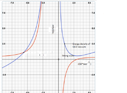
Figure 2: Summing graphs of strong gravitational gluodynamics.

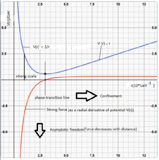
Figure 3: Graphs of pure Yang-Mills potential (in blue) and Yang-Mills-Gravity force (in red).

IX.1 Energy density of QCD vacuum

The scale invariance of the strong gravity is broken at $\Lambda_{QCD}\approx 1GeV$ (ASCS . P. 324). Hence the associated distance scale would be given as $r_{g}=G_{f}=1GeV^{-1}.$ In terms of the observable hadronic radius (see Eq.(87)), we have $r_{h}=10GeV^{-1}=1.972\times 10^{-15}m=1.972$ $fm.$ The QCD potential at this distance scale is given as $V_{YM}^{eff}=2.495761GeV$ from the Fig.3, and the energy density ($\varepsilon$) of the QCD vacuum is calculated as:

$$\varepsilon=\frac{V_{YM}^{eff}}{(r_{h})^{3}}=\frac{2.495761GeV}{(1.972)^{3}fm^{3}}=0.325GeV\text{ }/\text{ }fm^{3}$$ (138)

Eq.(138) is to be compared with the value calculated from the Lattice QCD ($\varepsilon\approx 0.33GeV$ $/$ $fm^{3}$) (HENG , P.54).

X Existence of Quantum Yang-Mills Theory on R⁴

The existence of quantum Yang-Mills theory on $R^{4}$ (with its characteristic mass gap) is one of the seven (now six) Millennium prize problems in mathematics that was put forward by Clay Mathematics Institute in 2000 TOGO27 . The problem is stated as follows:

Prove that for any compact simple gauge group $G=SU(N)$, a fully renormalized quantum Yang-Mills theory exists on $R^{4}$ and has a non-vanishing mass gap.

X.1 Solution-plan

The first thing to note here is that Yang-Mills theory is a non-abelian gauge theory, and the idea of a gauge theory emerged from the work of Hermann Weyl TOGO27A (the same Weyl that formulated the Weyl’s action that was used in the formulation of strong gravity theory, based on the Weyl-Salam-Sivaram’s approach ASCS ).

The Maxwell’s theory of electromagnetism is one of the classical examples of gauge theory. In this case, the gauge symmetry group of the theory is the abelian group $U(1)$. If $A$ designates the $U(1)$ gauge connection (locally a one-form on spacetime), then the potential of the field is the linear two-form $F=dA$. To formulate the classical version of the Yang-Mills theory, we must replace the gauge group $U(1)$ of electromagnetism by a compact gauge group $SU(N)$, and the potential arising from the field would be a generalized form of the Maxwell’s: $F=dA+A\Lambda A$. This formula still holds at the quantum level of the theory because Yang-Mills field shows quantum behavior that is very similar to its classical behavior at short distance scales (TOGO27 , P.1-2). However, the Maxwell’s theory must be replaced by its quantum version (i.e. QED; photon-electron interaction), and the nonlinear part ($A\Lambda A$) must now describe the self-interaction of gluons (which is the source of nonlinearity of the theory). The fact that the physics of strong interaction is described by a non-abelian gauge group $G=SU(3)$ (i.e. QCD), suggests immediately that the potentials of the four-dimensional quantum Yang-Mills field must be the sum of the linear QED ($dA$) and nonlinear QCD ($A\Lambda A$) potentials at quantum level. Thus the first composite hurdle for any would-be solution of the problem to cross is to: (1) obtain $QED+QCD$ potential at short distances with a single unified coupling constant. (2) The two potentials must perfectly explain the individual physics of QED and QCD at the quantum scale. (3) The two potentials must be obtained from a four-dimensional quantum gauge theory. To surmount this composite hurdle, one must first of all establish the existence of four-dimensional quantum gauge theory with gauge group $G=SU(N)$, and then every other thing will follow naturally.

X.1.1 Jaffe-Witten Existence Theorem (TOGO27 ,P.6)

The official description of this (i.e. Yang-Mills existence and mass gap) problem was put forward by Arthur Jaffe and Edward Witten. Their existence theorem is briefly paraphrased as follows: The existence of four-dimensional quantum gauge theory (with gauge group $SU(N)$) can be established mathematically, by defining a quantum field theory with local quantum field operators in connection with the local gauge-invariant polynomials, in the curvature $F$ and its covariant derivatives, such as $TrF_{ij}F_{kl}(x)$. In this case, the correlation functions of the quantum field operators should be in agreement with the predictions of perturbative renormalization (i.e. the theory must have UV regularity) and asymptotic freedom (i.e. the weakness of strong force at extremely short-distance scale); and there must exist a stress tensor and an operator product expansion, admitting well-defined local singularities predicted by asymptotic freedom.

By using the eye of differential geometry, we observed that the solution to the problem is concealed in the mathematical structures rooted in the differential geometry . In other words, the above-stated existence theorem is the mathematical description of the strong gravity formulation.

X.1.2 R${}^{4}-$Weyl-Salam-Sivaram TheoremASCS

The Weyl-Salam-Sivaram theorem is in fact the geometrical interpretation of the Jaffe-Witten existence theorem. In the following, the local quantum field operators are the two strong tensor fields ($G_{\mu}^{a}(x)$ and $G_{\nu}^{b}(x);$ two gluons forming double-copy construction) used to construct the spacetime metric in the section III of this paper. These local quantum fields have a direct connection (via $g=\det(G_{\mu}^{a}G_{\nu}^{b}\eta_{ab})$) with the gauge-invariant  local polynomials in the curvature $C$ and its covariant derivatives: $\sqrt{-g}C_{\alpha\beta\gamma\delta}C^{\alpha\beta\gamma\delta}(x)$. Note that ”$Tr$” in the Jaffe-Witten existence theorem denotes an invariant quadratic form on the Lie algebra of group $G$. Similarly, $\sqrt{-g}$ in the Weyl-Salam-Sivaram theorem denotes an invariant quadratic form on the gauge group $SU(3).$ The correlation function in this case is nothing but the spacetime metric ($g_{\mu\nu}(x)$) constructed out of the two local quantum fields ($G_{\mu}^{a}(x)$ and $G_{\nu}^{b}(x)$), and used as a function of the spatial cum temporal distance between these two random variables (gluons). We have painstakingly demonstrated that this spacetime metric agrees, at short distance scales, with the predictions of asymptotic freedom (i.e. the weakness of strong force at extremely short distance scales (see section IX)) and perturbative renormalization (i.e. the existence of UV regularity of the theory at short distances; the theory should be able to regularize its own divergences at extremely short distance scales, say, $r=0$ (see subsection C of section VIII)). There also exist a stress energy-momentum tensor (Eq.(17)), and field product expansion (Eq.(18)), having local singularities encoded in the three-dimensional Dirac delta functions (Eqs. (19) and (30)) predicted by asymptotic freedom. Overall the broken-scale-invariant Weyl action (Eq.(27)) is the required perturbative four-dimensional quantum gauge field theory with its inherent gauge group $SU(3)$ that gives rise to color/Casimir factor $4/3$ (Eq.(107)). However, for this statement to be valid the theory must possess both QED and QCD potentials (i.e. $F=dA+A\Lambda A$). Happily, the theory does possess these potentials with a single coupling constant (see Eqs. (106), (110), (111) and (113)).

The fact that the scale invariance of Weyl action is broken at the strong scale $\Lambda_{QCD}=G_{f}^{-1}\approx 1GeV$ (ASCS , P.324) $-$ which is equal to its dynamical chiral symmetry breaking scale TOGO26 $-$ is a clear indication of the existence of proton as the fundamental hadron of the theory. In this case, one must therefore investigate the ground state (neutron state) of the proton state using isospin symmetry. But for this to be possible, the gauge group that describes isospin symmetry must exist within the framework of the theory. This is where custodial symmetry (Eq.(77)) kicks in. The vector subgroup of custodial symmetry is in fact the isospin symmetry: $SU(2)_{L}\times SU(2)_{R}\longrightarrow SU(2)_{V}$ TOGO28 . This isospin symmetry then demands that the Hamiltonian ($H$) of proton-neutron state must be zero. However, the near mass-degeneracy of the neutron and proton in the $SU(2)$ doublet representation points to an approximate isospin symmetry of the Hamiltonian describing the strong interaction DGR ; CITZ . The mass gap in this picture is nothing but the energy difference between the two sub-states of the proton-neutron configuration: $m_{gap}=m_{n}-m_{p}\approx 1.29MeV.$ Hence the mass formula of QCD (Eq.(93)) and the stable Higgs boson mass (see next section) must be expressed in terms of this mass gap.

Conclusively, the two gauge groups that are needed to accurately describe the solution to this Millennium prize problem are $\ SU(3)-$ for the establishment of the existence theorem$-$ and $SU(2)-$ for describing the mass gap of the solution.  Hence, the Weyl-Salam-Sivaram existence theorem of strong gravity puts quantum gauge field theory (QFT) on a solid mathematical footing of the differential geometry; in this sense, QFT is a full-fledged part of mathematics.

XI Stability of Vacuum: A hint for Planck scale physics from $m_{H}=126GeV$

The 126GeV Higgs mass seems to be a rather special value, from all the a priori possible values, because it just at the edge of the mass range implying the stability of Minkowski vacuum all the way down to the Planck scale EFEMI3 . If one uses the Planck energy ($G_{N}^{-1}\approx 10^{19}GeV$) as the cutoff scale, then the vacuum stability bound on the mass of the Higgs boson is found to be 129GeV. That is, vacuum stability requires the Higgs boson mass to be $m_{H}=129GeV$ EFEMI4 . A new physics beyond SM is thus needed to reconcile the discrepancy between 126GeV and 129GeV mass of Higgs boson. The first thing to observe here is that the vacuum stability bound on the mass of Higgs boson ($m_{H}=129GeV$) has exactly the same ”number-structure” with the values that we have been working with in this paper.

By using Eq.(93), we can write

$$m_{H}=const.\times m$$ (139)

Comparing the energy scale of the pure Yang-Mill propagator in the Eq.(29) ($k^{-2}=1\times 10^{17}GeV$) with the Planck scale ($\approx G_{N}^{-1}\approx 10^{19}GeV$) shows a magnitude difference of $10^{2}.$ By using this value as our constant (i.e. $const.=\frac{G_{N}^{-1}}{k^{-2}}$), we get exactly $m_{H}=129GeV$:

$$m_{H}=m\left(\frac{G_{N}^{-1}}{k^{-2}}\right)=129GeV$$ (140)

Eq.(140) is very important because: (1) it shows the coupling of Higgs mass ($m_{H}$) to the fundamental mass, and mass gap of the QCD vacuum ($m=1290MeV=10^{3}\times m_{gap}$). (2) It connects Higgs mass to the Planck energy scale. To show the vacuum stability property of the Eq.(140), we eliminate the fundamental mass of the QCD vacuum by using the value of critical temperature from Eq.(89) ($T\equiv m=10T_{c}$):

$$m_{H}=T\left(\frac{G_{N}^{-1}}{k^{-2}}\right)=129GeV$$ (141)

Obviously, $T>T_{c}$ (see subsection A of section VII). This is the well-known vacuum stability condition in the second-order phase transition theory; while the condition for vacuum instability is $T<T_{c}$ (see FRAG and the references therein).

The mass range of the Higgs boson that would allow the stability of vacuum is given as IATO :

$$123GeV\leq m_{H}\leq 129GeV$$ (142)

By taking the average value of Eq.(142), we have

$$m_{H}^{avg}=\frac{123GeV+129GeV}{2}=126GeV$$ (143)

Clearly, 126GeV Higgs mass is special because it just at the midpoint of the mass range that guarantees the stability of the vacuum.

XII The Enigmatic Neutrino

”A cosmic mystery of immense proportions, once seemingly on the verge of solution, has deepened and left astronomers and astrophysicists more baffled than ever. The crux …is that the vast majority of the mass of the universe seems to be missing.” - William J. Broad (1984)

”A billion neutrinos go swimming in heavy water:  one gets wet.” - Michael Kamakana

Studying the properties of neutrinos has been one of the most exciting and challenging activities in particle physics and astrophysics ever since Pauli, ”the unwilling father” of neutrino, proposed their existence in 1930 in order to find the desperate remedy for the law of conservation of energy, which appeared to be violated in $\beta-$decay processes. Since then, many hidden facts about neutrinos have been unveiled step by stepFBP ; SWJ . In spite of their weakly interacting nature, we have so far gathered an avalanche of knowledge about neutrinos. From the neutrino oscillation experiments (an effort that has been duly awarded the 2015 Nobel prize in physics TKAB ), we learned that there are two major problems that plague neutrino physics:

(1) Determination of the absolute masses of neutrinos. The results from the neutrino oscillation experiments have confirmed the massive nature of neutrino. However, this confirmation provides a crack in the foundation of the Standard Model (SM) of particle physics, because SM treats neutrinos as massless particles. This disagreement between SM and experimental results (which opens a new door to the physics beyond SM) constitutes what is called ”neutrino mass problem”TKAA7 ; ABMD3 ; ASNE ; KEG ; PAD ; YABD ; FANE ; JAHN .

(2) Another major problem in the neutrino physics that is somehow related to the one above-mentioned, is to establish whether the neutrinos with definite masses $m_{k}$ are Dirac particles (with particles and antiparticles being different objects thereby conserving the lepton number) or Majorana particles (with particles and antiparticles being the same thereby violating lepton number). An experimental distinction between these two seems to be much more complicated than the confirmation of non-vanishing mass of the neutrino. These are the two major problems in neutrino physics that have hitherto defied all solutions.

Based on the formulation of the strong gravity theory (that hadronic interactions become weak in strength at small invariant separation), we assert that the absolute masses of neutrinos are actually calculable. More importantly, we will demonstrate, in this section, that neutrinos are Majorana particles! In few lines, we explain the theoretical properties of neutrino’s nature that form the basis for using the strong gravity formulation.

(i) All types of neutrino participate in weak nuclear and gravitational interactions with ordinary matter YVKO . This means that their physics can be explained by using a gas of weakly coupled particles system (a configuration that we used to solve the problem of asymptotic freedom (i.e., calculation of the dimensionless strong coupling constant at the starting point of QCD evolution in this paper)). The fact that strong gravity combines strong nuclear force (which becomes weak at extremely short distance scale: $r\ll\Lambda_{QCD}^{-1}$) and gravitational force into one unified force makes the determination of neutrino masses possible within the framework of massive spin-2 field theory with $D=5$: note that the Lagrangian of the Majorana neutrino is valid only when $D=5$.

(ii) Majorana neutrino Lagrangian possesses symmetry axis / CP-symmetry (TOGO19 , P. 203-205).

These two points form the basis of our solution-plan for solving the neutrino mass problem. This approach shows a compelling interplay between gravitation and principle of linear superposition of different mass eigenstates of neutrino as alluded to in DVACB .

XII.1 Effective Majorana Mass Matrix

Since the Majorana neutrino has only left-handed chiral field $\nu_{L},$ which is present in the SM, it is therefore natural to ask if it possible for SM neutrinos to have Majorana masses. The simple answer is that it is not possible, due to the fact that the left-handed chiral field $\nu_{L}$ has weak isospin triplet with hypercharge $Y=-2.$ The fact that SM does not contain any weak isospin triplet with $Y=2$ clearly  shows that it is not possible to have a renormalizable Lagrangian term which can generate Majorana neutrino masses (TOGO19 , P. 205).

However, the lowest dimensional Lagrangian which could generate Majorana neutrino masses that one can construct with the SM fields, respecting the SM symmetries, is the lepton number violating Lagrangian (with $D>4$) (TOGO19 , P. 216):

$$\mathcal{L}_{d}=M_{X}^{4-D}\underset{\alpha\beta}{\sum}g_{\alpha\beta}(L_{\alpha L}^{{}^{\prime}T}\tau_{2}\Phi)C^{{\dagger}}(\Phi^{T}\tau_{2}L_{\beta L}^{{}^{\prime}})+H.c.$$ (144)

where $M_{X}$ is a heavy mass ( of a single color triplet Higgs scalar ) characteristic of the symmetry-breaking scale of the high-energy unified theory, $D$ is called a dimension-D operator and its value in this case is $D=5.$ $g_{\alpha\beta}$ is a yet-unknown symmetric $3\times 3$ matrix of coupling constants. With $D=5,$ Eq.(144) becomes

$$\mathcal{L}_{5}=\frac{1}{M_{X}}\underset{\alpha\beta}{\sum}g_{\alpha\beta}(L_{\alpha L}^{{}^{\prime}T}\tau_{2}\Phi)C^{{\dagger}}(\Phi^{T}\tau_{2}L_{\beta L}^{{}^{\prime}})+H.c.$$ (145)

The electroweak symmetry breaking VEV ($=\upsilon=246GeV$ DBAL ) of the Higgs field leads to the Majorana neutrino mass term(TOGO19 , P. 216);

$$\mathcal{L}_{mass}^{M}=\frac{1}{2}\frac{\upsilon^{2}}{M_{X}}\underset{\alpha\beta}{\sum}g_{\alpha\beta}\text{ }\nu_{\alpha L}^{{}^{\prime}T}C^{{\dagger}}\nu_{\beta L}^{{}^{\prime}}+H.c.$$ (146)

From Eq.(146),  the Majorana mass matrix has elements (TOGO19 , P. 216)

$$M_{\alpha\beta}^{L}=\frac{\upsilon^{2}}{M_{X}}\text{ }g_{\alpha\beta}$$ (147)

with (TOGO19 , P. 208)

$$M_{\alpha\beta}^{L}=M_{\beta\alpha}^{L}$$ (148)

Eq.(148) is the reason why the $g_{\alpha\beta}$ matrix must be symmetric. With $\alpha=\beta=0,1,2$, Eq.(147) reduces to

$$M_{00}^{L}=\frac{\upsilon^{2}}{M_{X}}\text{ }g_{00}$$ (149)

$$M_{11}^{L}=\frac{\upsilon^{2}}{M_{X}}\text{ }g_{11}$$ (150)

$$M_{22}^{L}=\frac{\upsilon^{2}}{M_{X}}\text{ }g_{22}$$ (151)

(It is worth noting that if all the diagonal elements of $g_{\alpha\beta}$ are all 1’s, then the Eqs. (147) and 149-151 reduce to Eq.(74).)

The gravitational potential ($g_{\mu\nu}$) which is capable of representing a combined gravitational and electromagnetic field outside a spherically symmetric material distribution is given as MIW ;

$$g_{\mu\nu}=\left(\begin{array}[c]{cccc}g_{00}&g_{01}&0&0\\ g_{10}&g_{11}&0&0\\ 0&0&g_{22}&0\\ 0&0&0&g_{33}\end{array}\right)$$ (152)

where

$$g_{00}=\frac{(1-\frac{m}{2r})^{2}}{(1+\frac{m}{2r})^{2}}+\frac{\zeta^{2}}{r(1+\frac{m}{2r})^{2}}$$ (153)

$$g_{01}=g_{10}=-\frac{\zeta(1+\frac{m}{2r})}{r^{1/2}}$$ (154)

$$g_{11}=(1+\frac{m}{2r})^{4}$$ (155)

$$g_{22}=g_{11}r^{2}$$ (156)

$$g_{33}=g_{22}\sin^{2}\theta=g_{11}r^{2}\sin^{2}\theta$$ (157)

The quantity $m$ represents an effective gravitational mass, and $\zeta$ is an electric-charge dependent parameter MIW . Since neutrinos are electrically neutral, we set $\zeta$ to zero: $\zeta=0.$ Hence Eq.(152) reduces to

$$g_{\mu\nu}=\left(\begin{array}[c]{cccc}g_{00}&0&0&0\\ 0&g_{11}&0&0\\ 0&0&g_{22}&0\\ 0&0&0&g_{33}\end{array}\right)$$ (158)

and

$$g_{00}=\frac{(1-\frac{m}{2r})^{2}}{(1+\frac{m}{2r})^{2}}$$ (159)

$$g_{01}=g_{10}=0$$

This matrix (Eq.158) has Euclidean space signature $++++.$ It’s worth noting that for us to impose Lorentz signature on the above matrix, we must invoke the Levi-Civita indicator  on the matrix to account for the special relativity in the limiting case, and to also transform the metric from 4 dimensions to 3+1 dimensions. It doesn’t matter whether we insert the Lorentz signature before or after solving the Eq.(158), due to the fact that it is a diagonalized matrix FIMMW .

The fact that Majorana neutrino Lagrangian preserves CP symmetry means that it possesses symmetry axis ($\theta=0$). The reason why Majorana neutrino Lagrangian preserves CP symmetry is that Majorana particles are invariant to CP transformation (because Majorana particle = Majorana antiparticle) (TOGO19 , P. 203-205).

Consequently (by setting $\theta=0$), Eqs.(157-158) reduce to

$$g_{33}=0$$ (160)

$$g_{\mu\nu}=\left(\begin{array}[c]{cccc}g_{00}&0&0&0\\ 0&g_{11}&0&0\\ 0&0&g_{22}&0\\ 0&0&0&0\end{array}\right)$$ (161)

Hence, Eq.(147) becomes

$$M_{\alpha\beta}^{L}=\frac{\upsilon^{2}}{M_{X}}\text{ }\left(\begin{array}[c]{cccc}g_{00}&0&0&0\\ 0&g_{11}&0&0\\ 0&0&g_{22}&0\\ 0&0&0&0\end{array}\right)$$ (162)

By solving Eq.(159) completely for mass $m$, we have

$$m=\frac{2r(1-g_{00}^{1/2})}{(1+g_{00}^{1/2})}$$ (163)

Multiplying Eq.(159) by $\frac{(1+\frac{m}{2r})^{2}}{(1+\frac{m}{2r})^{2}}$ and solve the resulting equation completely for mass $m$;

$$m=\pm 2r[1-(g_{11}g_{00})^{1/2}]^{1/2}$$ (164)

where $\pm$ sign  in Eq.(164) leads to the same result. By comparing Eq.(163) with Eq.(164), we get

$$g_{11}=\frac{1}{g_{00}}\left[1-\frac{(1-g_{00}^{1/2})^{2}}{(1+g_{00}^{1/2})^{2}}\right]^{2}$$ (165)

Since our calculated value for $g_{00}$ is $g_{00}=0.1797,$ thus Eqs.(156) and (165) reduce to

$$g_{11}=3.8922$$ (166)

$$g_{22}=3.8922r^{2}$$ (167)

We now look for an ingenious way to eliminate $r^{2}$ in Eq.(167). It is tempting to straightforwardly use unit sphere formalism but this direct approach will not work because $M_{\alpha\beta}^{L}$ is a linear superposition of three different neutrino masses, albeit from the same source. The best mathematical approach that we can use to circumvent this problem is the 3-sphere formulation (note that this approach is anchored on the fact that 3-sphere is a sphere in 4-dimensional Euclidean space) GEOLE ; MAAPE :

$$r^{2} =\overset{3}{\underset{i=0}{\sum}}(x_{i}-C_{i})^{2}=(x_{0}-C_{0})^{2}+(x_{1}-C_{1})^{2}+$$

$$(x_{2}-C_{2})^{2}+(x_{3}-C_{3})^{2}$$ (168)

We turn Eq.(168) on its head by using it to represent three spheres (representing three types of neutrino) with common origin. This reduces Eq.(168) to ordinary linear superposition of three spheres (in two-dimension, they reduce to circles) with common origin / source. Suppose we further impose the condition that the common origin is centred at zero (i.e., $x_{0}-C_{0}=0$), then Eq.(168) reduces to

$$r^{2}=\overset{3}{\underset{i=1}{\sum}}(x_{i}-C_{i})^{2}=(x_{1}-C_{1})^{2}+(x_{2}-C_{2})^{2}+(x_{3}-C_{3})^{2}$$ (169)

where $x_{1}-C_{1},$ $x_{2}-C_{2}$ and $x_{3}-C_{3}$ are the radii of the spheres. By using unit sphere formalism individually on the three sphere, Eq.(169) reduces to

$$r^{2}=\overset{3}{\underset{i=1}{\sum}}(x_{i}-C_{i})^{2}=3$$ (170)

Thus, Eq.(167) becomes

$$g_{22}=11.6766$$ (171)

and Eq.(161) reduces to

$$g_{\mu\nu}=\left(\begin{array}[c]{cccc}0.1797&0&0&0\\ 0&3.8922&0&0\\ 0&0&11.6766&0\\ 0&0&0&0\end{array}\right)$$ (172)

With $M_{X}=1.63\times 10^{16}GeV$ (see subsection C of section VI) and $\upsilon=246GeV$ DBAL , $\frac{\upsilon^{2}}{M_{X}}=3.7meV$ (see Eq.(79)).

Hence Eqs.(149-151) reduce to

$$m_{0}=0.665meV$$ (173)

$$m_{1}=14.401meV$$ (174)

$$m_{2}=43.203meV$$ (175)

where $m_{0}\equiv M_{00}^{L},$ $m_{1}\equiv M_{11}^{L},m_{2}\equiv M_{22}^{L}$ and $m_{3}\equiv 0.$ And Eq.(162) reduces to

$$M_{\alpha\beta}^{L}=3.7meV\left(\begin{array}[c]{cccc}0.1797&0&0&0\\ 0&3.8922&0&0\\ 0&0&11.6766&0\\ 0&0&0&0\end{array}\right)$$ (176)

For the purpose of book-keeping, we set $m_{0}\equiv m_{1},$ $m_{1}\equiv m_{2}$ and $m_{2}\equiv m_{3}$. It is evident from Eqs.(173-175) that $m_{1}<m_{2}<m_{3},$ which is clearly a Normal Mass Hierarchy signature. The validity of which can also be confirmed by considering the approach of M. Kadastik et al MKMR .

$$N_{1}=\frac{-m_{1}^{2}+m_{2}^{2}+3m_{3}^{2}}{2m_{1}^{2}+m_{2}^{2}}$$ (177)

with

$$N_{1} >1\rightarrow\text{ normal mass hierarchy}$$

$$N_{1} <1\rightarrow\text{ inverted mass hierarchy}$$

$$N_{1} \approx 1\rightarrow\text{ degenerate masses}$$ (178)

Taking the values of $m_{1},m_{2},$ and $m_{3}$ from Eqs.(173-175), Eq.(177) gives the value $N_{1}\approx 28,$ which satisfies the criterion of normal mass hierarchy in Eq.(178).

The  mass-squared difference is defined mathematically as

$$\Delta m_{ij}^{2}=m_{i}^{2}-m_{j}^{2}$$ (179)

where $i>j.$ Based on the Eq.(179) (and taking into account Eqs.(173-175)), we have the following equations:

$$\Delta m_{21}^{2}=m_{2}^{2}-m_{1}^{2}=2.06\times 10^{-4}eV^{2}$$ (180)

$$\Delta m_{31}^{2}=m_{3}^{2}-m_{1}^{2}=1.87\times 10^{-3}eV^{2}$$ (181)

$$\Delta m_{32}^{2}=m_{3}^{2}-m_{2}^{2}=1.57\times 10^{-3}eV^{2}$$ (182)

XII.1.1 Experimental Test

(1)  The combined results of all solar experiments with Super-Kamiokande-I zenith spectrum and KamLAND data give $\Delta m_{sol}^{2}=\Delta m_{21}^{2}=2\times 10^{-4}eV^{2}$ at $99.73\%$ C. L.HNWJ . This experimental value is compatible with our Eq.(180): Thus confirming the validity of our $m_{1}$ and $m_{2}$ values.

(2) From the atmospheric neutrino oscillation experiments, the bound on the mass of the heaviest neutrino is $m_{3}\gtrsim 40meV$ HVKLK . This value experimentally confirms our value in the Eq.(175). We therefore assert that the values of our $m_{1},m_{2}$ and $m_{3}$ conform with the experimental data.

XII.2 Observational Test

The energy density of light massive neutrinos is given as (TOGO19 , P. 590-591):

$$\Omega_{\nu}^{0}h^{2}=\frac{\overset{3}{\underset{i=1}{\sum}}m_{i}}{94.14eV}$$ (183)

where $\Omega_{\nu}^{0}h^{2}$ is the neutrino energy density (which is also known as the Gershtein-Zeldovich limt or Cowsik-McClelland limit) and $\overset{3}{\underset{i=1}{\sum}}m_{i}$ is the sum of the three active neutrino masses. From Eqs.(173-175), $\overset{3}{\underset{i=1}{\sum}}m_{i}=0.058269eV.$ To obtain an accurate result, we must convert the calculated value of sum of the neutrino into two decimal places in conformity with the denorminator of Eq.(183). Thus

$$\overset{3}{\underset{i=1}{\sum}}m_{i}\approx 0.06eV$$ (184)

Consequently,

$$\Omega_{\nu}^{0}h^{2}\approx 0.00064$$ (185)

Eqs.(184) and (185) are the fiducial parameter values that have been taken to be valid for the background Cosmology to be consistent with the most recent cosmological measurements JBDH . Here, it turns out that the South Pole Telescope (SPT) cluster abundance is lower than preferred by either the WMAP9 or Planck+WMAP9 polarization data for the Planck base $\Lambda CDM$ model; but assuming a normal mass hierarchy for the sum of of the neutrino masses with $\sum m_{\nu}\approx 0.06eV$ (TOGO18 , P.237 & 239) the data sets are found to be consistent at the $1.0\sigma$ level for WMAP9 and $1.5\sigma$ level for Planck+WMAP9 SBDCQ . Obviously, our calculations confirm that the Planck base $\Lambda CDM$ model’s prediction of sum of the neutrino masses is correct.

XIII Dark Energy

For the strong gravity theory to be a complete theory of QCD and gravity, it must be tested okay at both small and large scale distances. The large distance ,here, is the cosmological scale where ”dark energy” is dominant $-$ Dark energy ($\rho$) is an unknown form of energy, which was invented to account for the acceleration of the expanding universe. The observed value (upper limit) of $\rho$ is $\rho^{observed}\approx(2.42\times 10^{-3}eV)^{4}$ AGRI $-$ A major outstanding problem is that most quantum field theories naively predict a huge value for the dark energy: the prediction is wrong by a factor of $10^{120}$ AGRI1 . The origin of the problem is now clear to us: Eqs.(118) and (120) clearly show that the energy-momentum tensor is related to the invariant (Weyl) Lagrangian density, but not to the total energy density of a vacuum, which is not operationally measurable, due to quantum fluctuations!

The energy density of any given system, such as the universe, is categorized into two parts: one is due to the true vacuum ($\rho$) and the other to the matter and radiation (pressure ($p$)) present in the system. These two types of energy density are related by the energy-momentum tensor $T_{\mu\nu}$ SW-2 :

$$T_{\mu\nu}=\text{ }\left(\begin{array}[c]{cccc}\rho&0&0&0\\ 0&-p&0&0\\ 0&0&-p&0\\ 0&0&0&-p\end{array}\right)$$ (186)

( Note that by putting Eq.(186) into Eq.(134), two things happen: (1) The energy density of the true vacuum becomes negative, meaning repulsive gravity and (2) the energy density of matter and radiation becomes positive, meaning attractive gravity. These two results are compatible with the observations. The gravity of ordinary matter/energy is always attractive, while the gravity of true vacuum (i.e., dark energy) is always repulsive.)

Since it has been observationally confirmed that the acceleration of the expanding universe is controlled by the energy density of true vacuum ($\rho$),but not by the matter/energy content of the universe, we can write (from Eq.(186))

$$T_{00}=\rho$$ (187)

By combining Eq.(120) with Eq.(187), we get Eq.(50):

$$\rho=g_{00}[E_{vac}]^{4}$$ (188)

Note that the Weyl Lagrangian density scales as $C_{\alpha\beta\gamma\delta}C^{\alpha\beta\gamma\delta}\sim[E_{vac}]^{4}$ (where $E_{vac}$ denotes the effective (Weyl) Lagrangian of the vacuum), due to the scale invariance of the Weyl’s action in the Eq.(7) (TOGO19 , P.206). To see the repulsive nature of the dark energy, we combine Eqs.(134) and (188) to get

$$G_{\mu\nu}=-8\pi G_{N}\text{ }\left(\begin{array}[c]{cccc}\rho&0&0&0\\ 0&0&0&0\\ 0&0&0&0\\ 0&0&0&0\end{array}\right)$$ (189)

where $G_{\mu\nu}\equiv R_{\mu\nu}-\frac{1}{2}g_{\mu\nu}$ $R$ is the Einstein’s tensor. The negative sign in the Eq.(189) is the hallmark of the repulsive nature of dark energy. It is to be noted that we have not invoked the presence of the famous cosmological constant ($\Lambda$) in the Eq.(134) because it is not needed for the expanding or contracting universe (TOGO18 , P.232). All what is needed for the accelerating expansion of the universe, as currently observed, is the Eq.(189); while the combination of the Eqs.(134) and (186) tell us that the universe will either expand (if the right-hand side of the Eq.(134) is negative ($\rho$)) or contract (if the right-hand side of the Eq.(134) is positive (p)). Albert Einstein was right after all: the introduction of the fudged factor ($\Lambda$) was his greatest blunder. You cannot out-einstein Einstein!

Using Eqs.(56) and (79), Eq.(188) becomes

$$\rho=(2.41\times 10^{-3}eV)^{4}$$ (190)

Obviously, Eq.(190) compares favorably with the upper bound value of the observed $\rho$ ($\rho^{observed}=(2.42\times 10^{-3}eV)^{4}$) AGRI .

It has long been suggested that the nonrelativistic massive neutrinos may give a significant contribution to the energy density (i.e. the so-called dark energy) of the universe (TOGO19 , P.590). This statement has been confirmed to be true via Eqs.(176) and (188): with $E_{vac}=\upsilon^{2}/M_{X}=3.7meV$.

We understand, of course, that the energy of vacuum is extremely large (due to quantum fluctuations) but the strong gravity and Majorana-neutrino Lagrangian (a conserved quantity that encodes the information about the dynamics of the universe) tell us that it is only the effective Lagrangian of the universe that is physically measurable (i.e. $\upsilon^{2}/M_{X}=3.7meV$).

XIV Dark Matter OR Leftover Yang-Mills-Gravity Force?

XIV.1 The Galaxy Rotation Problem (GRP)

The GRP is the inconsistency between the theoretical prediction and the observed galaxy rotation curves, assuming a centrally dominated mass associated with the observed luminous material. The direct computation of mass profiles of galaxies from the distribution of stars and gas in spirals and mass-to-light ratios in the stellar disks, utterly disagree with the masses derived from the observed rotation curves using Newtonian force law of gravity. Based on the Newtonian dynamics, most of the mass of the galaxy had to be in the galactic bulge near the center, and that stars and gas in the disk portion should orbit the center at decreasing velocities with increasing radial distance, away from the galactic center V.R ; ECO ; VTR : This is achieved by equating the centripetal force experienced by the orbiting gas/stars to the Newton force law (TOGO18 , P.241):

$$F_{c} =F_{N},$$

$$v =\sqrt{\frac{G_{N}\text{ }M}{r}}\implies v(r)\propto 1/\sqrt{r}$$ (191)

where $v$ is the speed of the orbiting star, $M$ is the centrally dominated mass of the galaxy and $r$ is the radial distance from the center of the galaxy.

However, the actual observations of the rotation curve of spirals completely disagree with the Eq.(191): the curves do not decrease in the expected inverse square root relationship. Rather, in most galaxies observed, one finds that $v$ becomes approximately constant out to the largest values of radial distance $(r)$ where the rotation curve can be measured (TOGO18 , P.241). A solution to this problem was to hypothesize the existence of a substantial invisible amount of matter to account for this inexplicable extra mass/gravity force that keeps the speed of orbiting stars/gas approximately constant for extremely large values of $r$.  This extra mass/gravity was dubbled ”dark matter” FKA .

Though dark matter is by far the most accepted explanation of the rotation problem, other alternatives have been proposed with varying degrees of success. The most notable of these alternatives is the Modified Newtonian Dynamics (MOND), which involves modifying the Newton force law by phenomenologically adding a small fudged factor $\alpha_{0}$:

$$F_{MOND}=\frac{G_{N}\text{ }Mm}{r^{2}}+\alpha_{0}$$ (192)

Within the central bulge of galaxy, the first term of the Eq.(192) dominates, and to the largest value of $r$ where the rotation curve can be measured (the domain of dark matter), the second term dominates. MOND has had a remarkable amount of success in predicting the flat rotation curves of low-surface-brightness galaxies, matching the Tully-Fisher relation of the baryonic distribution, and the velocity dispersions of the small orbiting galaxies of the local group 22 .

The ensuing fundamental question here is: Do we really need to modify Newtonian dynamics and Einstein’s GR before we could account for this extra gravitational force with no ”origin”? The answer is a big No! The two theories are fantastically accurate in their respective domains of validity. But the core of the problem is that we assumed that both theories should be valid at all distance scales (from particle physics scale (say, Planck scale) to the edge of the Universe); but the irony is that they are not. It turns out that in order to solve GRP, one needs a force law that is valid for all distance scales. This is where BCJ construction kicks in. As we have painstakingly demonstrated (by obtaining Eqs.(106) and (134) from Eq.(27)) , the major conclusion of double copy construction is the existence of gauge/gravity duality. This duality property led to the formulation of the Yang-Mills-Gravity (YM) force in the Eq.(137). A close perusal of Eqs.(137) and (192) shows that both equations are essentially the same; and that Eq.(137) explains the universal rotation curve perfectly, by producing a flatly stable curve at large values of $r$ (see red curve of the Fig.3) $-$ (a universal rotation curve can be expressed as the sum of exponential distributions of visible matter that reduce to zero with large values of $r$ away from the center of galaxy, and spherical dark matter halo (just like $\sigma$ in the Eq.(137)) that tapers to flat rotation curve with constant speed and gravitational force 45 ) $-$ Hence, the deep significance of structure of the Eq.(137) to cosmology is not accidental but fundamental to the evolutionary histories of our universe.

As pointed out by V. de Sabbata and C. Sivaram, a deviation from the Newton’s inverse square law can arise naturally from $R+R^{2}$ theory (such as strong gravity theory), whose solution gives a Newtonian/Coulomb potential and a Yukawa term (VDS , P.4). Thus it is natural to investigate the behavior of the Eq.(137) on a cosmological scale. Of course, Eq.(137) tapers to $\sigma$ on the cosmological scale:

$$F_{YMG}=0.299GeV^{2}=2.449\times 10^{5}N$$ (193)

with mass ($M_{g}$)

$$M_{g}=\sqrt{F_{YM}}=546.809MeV$$ (194)

As a result of the Eqs.(137) and (194), the following facts emerge: (1) empty space/vacuum is permeated with constant-attractive-gravitational force (dark matter) with mass $M_{g}=546.809MeV$. (2) The dark matter is stable on cosmological time scales due to the flat curve property of $M_{g}$ for $r\longrightarrow\infty$ (see red curve in the Fig.3). (3) Newtonian dynamics and Einstein’s GR need no modifications. (4) MOND is phenomenologically correct and happens to be compatible with YMG force law.

XV Repulsive Gravity and Cosmic Inflation

It is true (from the Eq.(137)) that $F_{YMG}$ can only get more repulsive as we probe shorter and shorter distances. As such, the separating distance between two gluons cannot taper to zero. This means that the theory ”realizes asymptotic freedom” because two gluons cannot sit on top of each other (i.e. separating distance $r=0$ is forbidden), hence they are almost free to move around due to the non-existent of attractve force at $r\ll\Lambda_{QCD}^{-1}$. This explanation is then carried by analogy into the construction of spacetime geometry. The fact that the spacetime metric ($g_{\mu\nu}$) is ab initio constructed out of the two entangled gluons (BCJ construction) means that spacetime cannot realize singularity (i.e. $r\neq 0$). From the foregoing, one is therefore forced to ask a fundamentally disturbing question: How did our universe ”begin”, or what existed ”before” the Big Bang?

A. C. Doyle famously claimed that ”once you eliminate the impossible, whatever remain, no matter how improbable, must be the truth.” In line with this quote, we posit that the behavior of the universe during the first fraction of a second ($t<10^{-44}s$) after the Big Bang can only be a matter for conjecture but we are certain that $t\neq 0$ and $r\neq 0$ due to the ever-increasing repulsive nature of $F_{YMG}$ as we probe short-distance scales. Hence, perhaps our universe had its origin in the ever-recurring interplay between expanding and contracting universe. We are sure of the former but the latter is highly unlikely, given the present behavior of dark energy and the ever-constant effective Lagrangian of the vacuum $\upsilon^{2}/M_{X}=3.7meV$.

The fact that most of the calculations done using Planck epoch parameters (i.e., Planck time, Planck energy and Planck length) conform to what is obtainable in nature strongly suggests that any epoch less than Planck epoch is operationally meaningless. Thus, a plausible theory can be constructed (starting from the Planck time $t=10^{-44}s$) by bringing the calculations done in the section IX of this paper to bear: After about $10^{-44}s$  (with Planck length $10^{-19}GeV^{-1}$) the repulsive gravity was $F_{YMG}=-2.6\times 10^{38}GeV^{2}(=-2.129\times 10^{44}N).$ This caused the universe to undergo an exponential expansion (due to the exponential nature of $F_{YMG}$). The exponential expansion lasted from $10^{-44}s$ after the Big Bang/Bounce to time $10^{4}GeV^{-1}(=6.6\times 10^{-21}s):$ this is the time that produced the stable-flat curve (red curve in the Fig.(3)), signaling the demise of the exponential era. Following this cosmic inflationary (exponential expansion) epoch, the dark matter $-$ which is nothing but the remnant of Yang-Mills-Gravity force, $F_{YMG}=2.449\times 10^{5}N$ $-$ dominates and the universe continues to expand but at a less rapid rate. The battle of supremacy between dark energy (repulsive gravity) and dark matter (attractive gravity) was won by dark energy during the time $t=6.6\times 10^{-21}s$: since dark energy is intimately connected to the spacetime metric itself (see Eq.(189)), it would have increased tremendously during the exponential expansion period, when the space increased in size by factor of $10^{23}(=10^{4}GeV^{-1}/10^{-19}GeV^{-1})$ in a small fraction of a second! The victory of dark energy over dark matter means that our universe will continue to expand ad infinitum: we are living in a runaway universe.

Another formal way of explaining the inflationary epoch (i.e. the vacuum-dominated universe approach) of the universe $-$ which makes the pre-existing universe scenario conceivable $-$ can be effected by using Fig.3. In this approach, it is believed that the universe passed through an early epoch of vacuum dominance (i.e. inflation), presided over by the varying potential energy (i.e. Eq.(113)) of the scalar field, called inflaton (TOGO19 , P.564). When the scalar field reached the minimum of the potential (which corresponds to the minimum of the potential curve (blue curve) in the Fig.3) exponential expansion ended. Based on the law of conservation of energy, the reduction in the potential energy (due to the rolling down of the inflaton from the top of the potential curve, i.e. the decaying of the inflaton field) generated hot (quark-gluon) plasma epoch (which later generated the matter and radiation epoch). So from then on, the Big Bang evolved according to the Standard Cosmological Model (TOGO19 , P.564); and governed by the Eqs.(105), (134), (189) and (193).

We conclude this section with the following facts: (1) The initial conditions of our universe are the Planck epoch parameters (i.e., Planck time, Planck energy and Planck length). (2) Inflationary theory is correct. (3) The expansion epoch of the universe consists two phases: (i) the exponential expansion (governed by $F_{YMG}=-2.129\times 10^{44}N$) and the normal accelerating expansion (governed by Eq.(189)).

XVI Conclusion

We have shown, in this paper, that the point-like theory of quantum gravity (strong gravity theory) is geometrically equivalent to the four-dimensional, nonlinear quantum gauge field theory (i.e. QYMT), and the Einstein General Relativity. The inherent UV regularity, BCJ and gauge-gravity duality properties of this renormalizable theory allowed us to solve four of the most difficult problems in the history of physics: namely, dark matter, existence of quantum Yang-Mills theory on $R^{4}$, neutrino mass and dark energy problems.

In any geometric field theory, all physical quantities and fields should be induced from one geometric entity (Weyl’s action) and the building blocks of the geometry used (2-gluon configuration/double-copy construction). This principle has been inspired by Einstein’s statement $-$ ”a theory in which the gravitational field and electromagnetic field do not enter as logically distinct structures, would be much preferable”$-$ and established in this paper. As we have demonstrated, this principle implies that the Weyl Lagrangian density used to construct the field equations of the strong gravity theory is composed of the building blocks (two gluons) of the geometry and their derivatives (in which the curvature arised in terms of derivatives of the dressed gluon field). In other words, Weyl Lagrangian is not constructed, a priori, from different parts (each corresponding to a certain field) as usually done. This makes strong gravity theory to pass the test of unification principle.

Acknowledgement

Mr. O.    F. Akinto is indebted to the Department of Physics, CIIT, Islamabad  and the National Mathematical Center Abuja, Nigeria  for their financial support.

References

- (1) C. J. Isham, A. Salam and J. Strathdee, ”2+ Nonet as Gauge particles for symmetry”, Phys. Rev. D8, 8 (1973).
- (2) A. Salam and J. Strathdee, ”Class of solutions for the strong-gravity equations”, Phys. Rev. D16, 8 (1977).
- (3) C. Sivaram and K. P. Sinha, ”Strong Spin-two Interaction and General Relativity”, Phys. Rep. (Rev. Sect. Phys. Lett.) 51, 3 (1979).
- (4) Dj. Sijacki and Y. Ne’eman, ”QCD as an effective strong gravity”, Phys. Lett. B247, 4 (1990).
- (5) Y. Ne’eman and Dj. Sijacki, ”Proof of pseudo-gravity as QCD approximation for the hadron IR region and Regge trajectories”, Phys. Lett. B276 (1992).
- (6) A. Salam and C. Sivaram, ” STRONG GRAVITY APPROACH TO QCD AND CONFINEMENT”, Mod. Phys. Lett. A8, 4 (1993).
- (7) I. Antoniadis and N. C. Tsamis, ”Weyl Invariance and the Cosmological Constant”, SLAC-PUB-3297, (1984).
- (8) K. S. Stelle, ”Renormalization of higher-derivative quantum gravity”, Phys. Rev. D16, 4 (1977).
- (9) E. Witten, ” Physical law and the quest for mathematical understanding”, Bulletin (New Series) of the American Mathematical Society, 40, 1 (2002).
- (10) J. Carson, A. Jaffe and A. Wiles (Editors),”The Millennium Prize Problems”, American Mathematical Society (2006).
- (11) B. I. Loffe, V. S. Fadin and L. N. Lipatov, ”Quantum Chromodynamics: Perturbative and Non-perturbative Aspects”, Cambridge University Press, New York (2010).
- (12) J. Goity, C. Keppel and G. Prezeau (Editors),”Proceedings of the 16th and 17th Annual Hampton University Graduate Studies”, World Scientific Publishing Co. Pte. Ltd (2001 & 2002).
- (13) J. Beringer et al., (Particle Data Group), Phys. Rev. D86, 010001 (2012).
- (14) H. Kawai, D. C. Lewellen and S. H. H. Tye, ”A relation between tree amplitudes of closed and open strings”, Nucl. Phys. B269, 1 (1986).
- (15) Z. Bern, J. J. M. Carrasco and H. Johansson, ”New Relations for Gauge-Theory Amplitudes”, Phys. Rev. D78, 085011 (2008).
- (16) Z. Bern, J. J. M. Carrasco and H. Johansson, ”Perturbative Quantum Gravity as a Double Copy of Gauge Theory”, Phys. Rev. Lett. 105, 061602 (2010).
- (17) American Physical Society, ”J. J. Sakurai Prize for Theoretical Particle Physics”, 2014 (Official site).
- (18) M. Chiodaroli, M. Gunaydin, H. Johansson and R. Roiban, ”Scattering amplitudes in N = 2 Maxwell-Einstein and Yang-Mills-Einstein supergravity”, JHEP 1501, 081 (2015); [arXiv:1512.09130 [hep-th]]; [arXiv: 1511.01740 [hep-th]].
- (19) H. Johansson and R. Roiban, ”Simplifying Multiloop Integrands and Ultraviolet Divergences of Gauge Theory and Gravity Amplitudes”, Phys. Rev. D85, 105014 (2012).
- (20) D. Hilbert, ”MATHEMATICAL PROBLEMS”, Bulletin (New Series) of the American Mathematical Society 37, 4 (2000).
- (21) F. Bissey, et al., ”Gluon flux-tube distribution and linear confinement in baryons”, Phys. Rev. D76, 114512 (2007); D. B. Leinweber, ”Visualizations of Quantum Chromodynamics”, Centre for the Subatomic Structure of Matter (CSSM) and Department of Physics, University of Adelaide, 5005 Australia (2003, 2004).
- (22) J. T. Ttrujillo, ”Weyl Gravity as a Gauge Theory”: All Graduate Theses and Dissertations, Paper 1951, Utah State University (2013).
- (23) S. Weinberg, ”Gravitation and Cosmology: Principles and Applications of the General Theory of Relativity”, Massachusetts Institute of Technology, John Wiley and Sons (1972).
- (24) B. S. DeWitt, ”In Relativity Groups and Topology”, ed. C. DeWitt and B. DeWitt (Gordon and Breach, 1964), P.719.
- (25) C. W. Misner, K. S. Thorne and J. A. Wheeler, ”Gravitation”, W. H. Freeman and Company, New York (1973).
- (26) Venzo de Sabbata and C. Sivaram, ”Fifth Force as a Manifestation of Torsion”, Int. J. Theor. Phys., 29, 1 (1990).
- (27) H. D. Politzer, ”Reliable Perturbative Results for Strong Interactions”, Phys. Rev. Lett. 30 (1973), 1346-1349; Phys. Rep. 14C, 129 (1974).
- (28) D. J. Gross and F. Wilczek, ”Ultraviolet Behavior of Non-Abelian Gauge Theories”, Phys. Rev. Lett. 30 (1973), 1343-1346; Phys. Rev. D8, 3633 (1973); D9, 980 (1974).
- (29) D. Gross, ”Methods in Field Theory”, ed. R. Balian and J. Zinn-Justin, North-Holland (1976).
- (30) W. Marciano and H. Pagels, ”Quantum chromodynamics”, Phys. Rep. 36C, 3 (1978).
- (31) J. W. Rohif, ”Modern Physics from a to z0”, Wiley, (1994).
- (32) D. Ashok and F. Thomas, ”Introduction to Nuclear and Particle Physics”, Wiley, (1994).
- (33) P. C. Riedi, ”Thermal Physics”, Macmillan Press Ltd, 1st ed. (1976).
- (34) O. Kiriyama, M. Maruyama and F. Takagi, ”Current quarks mass effects on chiral phase transition of QCD in the improved ladder approximation”, Phys. Rev. D62, 105008 (2000).
- (35) S. E. Rugh and H. Zinkernagel, ”The quantum vacuum and cosmological constant problem”, Studies in History and Philosophy of Science Part B33, 4 (2002).
- (36) L. Zhou, M. Weixing and L. S. Kisslinger, ”Theoretical prediction of cosmological constant in Veneziano ghost theory of QCD”, J. Mod. Phys. 3 (2012).
- (37) F. R. Urban and A. R. Zhitnitsky, ”The cosmological constant from the QCD Veneziano ghost”, Phys. Lett. B688, 9 (2010).
- (38) S. Weinberg, ”The cosmological constant problem”, Rev. Mod. Phys. 61, 1 (1998).
- (39) A. H. Mueller, Phys. Rep. 73C (1981) 237; A. J. Buras, Rev. Mod. Phys. 52 (1980) 199; S. J. Brodsky, T. Huang, G. P. Lepage, SLAC-PUB-2868, ”Quarks and Nuclear Forces”, Springer, Vol. (100), (1982).
- (40) G. P. Lepage and S. J. Brodsky, ”Exclusive processes in perturbative quantum chromodynamics”, Phys. Rev. D22, 2157 (1980).
- (41) A. Jaffe, G. Parisi and D. Ruelle (Editors),” Workshop on Non-perturbative Quantum Chromodynamics”, Birkhauser Boston, Inc. (1983).
- (42) S. Bethke, G. Dissertori and G. P. Salam, ” Quantum Chromodynamics”, Princeton University Press (2012).
- (43) V. G. Krivokhijine, A. V. Kotikov, ”A systematic study of QCD coupling constant from deep inelastic measurements”, Physics of Atomic Nuclei, 68, 11 (2005); [arXiv:0108224 [hep-ph]] (2001).
- (44) A. Pich, ”Effective Field Theory”, Elsevier Science B. V. (2008), P.11.
- (45) H. Georgi and M. Machacek, ”Doubly charged Higgs bosons”, Nucl. Phys. B262, 3 (1985); M. A.S. Kanemura, M. Kikuchi and K. Yagyu, Phys. Lett. B714, 279 (2012).
- (46) K. A. Olive et al. (Particle Data Group), ”Particle Physics Booklet”, Chin. Phys. C38, 09001 (2014) P.221.
- (47) C. Giunti and C. W. Kim, ”Fundamental of Neutrino Physics and Astrophysics”, Oxford University Press (2007) P.207.
- (48) R. A. Diaz, D. Gallego and R. Martinez, Int. J. Mod. Phys. A22 (2007), 1849-1874.
- (49) Nikolai Kochelev and Dong-Pil Min, ”Role of glueballs in non-perturbative quark-gluon plasma”, Phys. Lett. B650 (2007), 239-243.
- (50) A. A. Khan, S. Aoki, et al., ”Light hadron spectroscopy with two flavors of dynamical quarks on the lattice”, Phys. Rev. D65, 054505 (2002).
- (51) Shu-Sheng Xu, et al., ”The chiral phase transition with a chemical potential in the framework of Dyson-Schwinger equations”, Phys. Rev. D91, 056003 (2015).
- (52) U. Aglietti, Phys. Lett. B281, 341 (1992); L. Trentadue, Act. Phys. Pol. B38 (2007) 11.
- (53) V. Gogokhia and G. G. Barnafoldi, ” The Mass Gap and its Applications”, World Scientific Publishing Co. Pte. Ltd (2012).
- (54) D. Griffiths, ”Introduction to Elementary Particles”, John Wiley & Sons (1987).
- (55) C. Itzykson and J. B. Zuber, ”Quantum Field Theory”, McGraw-Hill (1980).
- (56) L. A. Gaume and M. A. V. Mozo, ”An Invitation to Quantum Field Theory”, Springer (2012).
- (57) P. J. Mohr, B. N. Taylor and A. B. Newell, ”CODATA recommended values of the fundamental physical constants”, Rev. Mod. Phys. 84, 1527 (2012).
- (58) R. Horsley, et al., Phys. Lett. B732 (2014).
- (59) J. Greensite, ” Lecture Notes in Physics 821: An Introduction to the Confinement Problem”, Springer (2011).
- (60) A. N. Ivanov, N. I. Troitskaya, M. Faber and M. Nagy, ”Chiral symmetry breaking in QCD with linearly rising confinement potential”, II Nuovo Cimento A107 (9), (1994).
- (61) M. Thomson, ”Modern Particle Physics”, Cambridge University Press, (2013).
- (62) A. Deur, S. J. Brodsky and G. F. de Teramond, ”The QCD Running Coupling”, SLAC-PUB-16448 (JLAB-PHY-16-2199) 2016, P.9; [arXiv:1604.08082 [hep-ph]].
- (63) D. V. Bugg (ed.),” Hadron Spectroscopy and the Confinement Problem”, NATO ASI Series B: Physics Vol. 353, Plenum Press New York and in NATO Scientific Affairs Division (1995).
- (64) S. M. Carrol, ”Spacetime and Geometry”, Addison-Wesley (2004).
- (65) A. V. Manohar and H. Georgi, ”Chiral quarks and the nonperturbative quark model”, Nucl. Phys. B234, 189 (1984).
- (66) J. M. Cornwall, ”What is the relativistic generalization of a linearly rising potential?”, Nucl. Phys. B127, 75(1977).
- (67) C. Gattringer and C. B. Lang, ”Qauntum Chromodynamics on the Lattice: An Introductory Presentation”, Springer (2010).
- (68) H. J. W. Muller and K. Schilcher, ”High-energy scattering for Yukawa potentials”, J. Math. Phys. 9 (1968); H. Yukawa, ”On the interaction of elementary particles”, Proc. Phys. Math. Soc. 17, 48 (1935); G. E. Brown and A. D. Jackson, ”The Nucleon-Nucleon Interaction”, North-Halland Publishing, Amsterdam (1976).
- (69) D. Scherfgen, htt:// www.derivative-calculator.net.
- (70) H. T. Ding,”Recent Lattice QCD results and phase diagram of strongly interacting matter”, Nucl. Phys. A931 (2014).
- (71) A. Jaffe and E. Witten, ”Quantum Yang-Mills Theory: Official problem description”, Clay Mathematics Institute (2000).
- (72) L. O’Raifeartaigh, ”The Dawning of Gauge Theory”, Princeton University Press, (1997); C. N. Yang and R. L. Mills, ”Conservation of isotopic spin and isotopic gauge invariance”, Phys. Rev. 96 (1954), 191-195.
- (73) T. Rodrigo and A. Ruiz (eds.), ”Proceedings of the XXIII International Meeting on Fundamental Physics”, World Scientific (1995).
- (74) E. Bertuzzo and C. Frugiuele, ”Natural SM-like 126GeV Higgs boson via non-decoupling D terms”, Phys. Rev. D93, 035019 (2016).
- (75) Bin He, N. Okada and Qaisar Shafi, ”125GeV Higgs, type III seesaw and gauge-Higgs unification”, Phys. Lett. B716 (2012).
- (76) F. Englert, ”Nobel Lecture: The BEH mechanism and its scalar boson”, Rev. Mod. Phys. 86, 843 (2014).
- (77) I. Antoniadis and D. Ghilencea (Editors), ”Supersymmetry After the Higgs Discovery”, Springer (2014).
- (78) F. Boehm and P. Vogel, ”Physics of Massive Neutrinos”, 2nd Ed., University of Cambridge Press (1987).
- (79) S. Wojcickl, ” Prospects in Neutrino Physics”, University of Stanford Press (1996).
- (80) T. Kajita and A. B. McDonald, ”The Nobel Prize in Physics 2015”, Nobel prize.org (2015).
- (81) A. Ereditato, T. Kajita and A. Masiero, New J. Phys. 9 (2007); T. Kajita, New J. Phys. 6, 194 (2004); J. Phys. G (Nucl. Part. Phys. 29, 1471 (2003)); J. Phys.(Conf. Ser. 308, 012003 (2011)); J. Phys. (Conf. Ser. 136, 022020 (2008)); T. Kajita, M. Ishitsuka, H. Minakata and H. Nunokawa, J. Phys.: Conf. Ser. 39, 332 (2006).
- (82) A. B. McDonald, New J. Phys. 6 (2004) 121; Phys. Scr. 2006, 10 (2006); J. Phys.(Conf. Ser. 173 (2009) 012002).
- (83) S. N. Ahmed, et al., (SNO Collaboration), Phys. Rev. Lett. (2003) 041801.
- (84) K. Eguchi, et al., (KamLAND Collaboration), Phys. Rev. Lett. 90 (2003) 021802.
- (85) P. Adamson, et al., (MINOS Collaboration), Phys. Rev. Lett. 107 (2011) 181802.
- (86) Y. Abe, et al., (Double Chooz Collaboration), Phys. Rev. Lett. 108 (2012) 131801; Phys. Rev. D86 (2012) 052008.
- (87) F. An. et al., (Daya Bay Collaboration), Phys. Rev. Lett. 108 (2012) 171803; F. An, et al., (Daya Bay Collaboration), Chin. Phys. C37 (2013) 011001.
- (88) J. Ahn, et al., (RENO Collaboration), Phys. Rev. Lett. 108 (2012) 191802.
- (89) Y. V. Kozlov, V. P. Martem ’yanov and K. N. Mukhin, Phys. 40 (1997) 8.
- (90) D. V. Ahluwalia and C. Burgard, Phys. Rev. D57 (1998) 8; Gen. Rel. Grav. 28 (1996).
- (91) D. Balin and A. Love, ”Supersymmetric Gauge Field Theory and String Theory”, CRC Press (1994).
- (92) M. I. Wanas, Int. J. Theor. Phys. 24 (1985); Stud. Cercet. Stin. Ser. Mat. 10 (2001); Int. J. Geom. Meth. Mod. Phys. Lett. A25 (2010).
- (93) F. I. Mikkhial, M. I. Wanas and G. G. L. Nashed, Astrophys. & Space Sci, 228 (1995): Proceedings of the fourth United Nations / European Space Agency Workshop, Cairo.
- (94) G. Lemaitre, ”Quaternions et e t espace elliptique”, Act. Pont. Acad. Sc., 12 (1948).
- (95) M. K. Peterson, ”Dante and the 3-Sphere”, Americ. J. Phys., 47 (1979) 12.
- (96) M. Kadastik, M. Raidal and L. Rebane, Phys. Rev. D77 (2008) 115023.
- (97) H. Nunokawa, W. J. C. Teves and R. Z. Funchal, Phys. Lett. B 562 (2003) 1.
- (98) V. Klapdor-Kleingrothaus, ” Seventy years of Double Beta Decay from Nuclear Physics to Beyond Standard Model Particle Physics”, World Scientific Publishing Co. Pte Ltd (2010); R. Mohaptra, A. Smirnov, Ann. Rev. Nucl. Part. Sci. 56 (2006) 569; M. Czakon, J. Gluza, J. Studnik and M. Zralek, Phys. Rev. D65 (2001) 5; P. Huber, ” Neutrino Theory”, Center for Neutrino Physics at Virginia Tech., International Workshop on Baryon and Lepton Number Violation, University of Massachusetts (2015).
- (99) J. Bielefeld, D. Huterer and E. V. Linder, JCAP05 (2015) 023; P. A. R. Ade, et al., Astron. & Astrophys. manuscript no. draft P1011 (2013) & manuscript no Planck Lensing (2015).
- (100) S. Bocquet, et al., APJ 799 (2015) 2.
- (101) B. P. L. Ward, ”CURRENT STATUS OF LHC PHYSICS: PRECISION THEORY VIEW”, ACTA PHYS POL B45, 7 (2014) P. 1632; A. G. Riess et al., Astron. J. 116, 1009(1998); S. Perlmutter et al., Astrophys. J. 517, 565 (1999); and references therein.
- (102) M. J. Luo, ”The cosmological constant problem and re-interpretation of time”, Nucl. Phys. B884 (2014).
- (103) V. Rubin and W. K. Ford, Jr, ”Rotation of the Andromeda Nebula from a Spectroscopic Survey of Emission Regions”, Astrophys. J. 159, 379 (1970); V. Rubin, N. Thonnard and W. K. Ford Jr, ”Rotational Properties of 21 SC Galaxies with a Large Range of Luminosities and Radii from NGC 4605 (R = 4kpc) to UGC 2885 (R = 122kpc)”, Astrophys. J. 238, 471 (1980).
- (104) E. Corbelli and P. Salucci, ”The extended rotation curve and the dark matter halo of M33”, Monthly Notices of the Royal Astron. Soc. 311, 2 (2000).
- (105) V. Trimble, ”Existence and nature of dark matter in the universe”, Annual Review of Astron. and Astrophys. 25 (1987).
- (106) F. Katherine, ”The Cosmic Cocktail: Three Parts Dark Matter”, Princeton University Press (2014).
- (107) S. S. McGaugh and W. J. G. de Block, ”Testing the Hypothesis of Modified Dynamics with Low Surface Brightness Galaxies and other Evidence”, Astrophys. J. 499, 1 (1998); S. S. McGaugh, ”Novel Test of Modified Newtonian Dynamics with Gas Rich Galaxies”, Phys. Rev. Lett. 106, 12 (2011); S. S. McGaugh and M. Milgrom, ”Andromeda Dwarfs in Light of Modified Newtonian Dynamics”, Astrophys. J. 766, 1 (2013).
- (108) P. Salucci and A. Borriello, ”The Intriguing Distribution of Dark Matter in Galaxies”, Lecture Notes in Physics 616: [arXiv:020345 [atroph-ph]].