Dealing with a large number of classes – Likelihood, Discrimination or Ranking?

Abstract

We consider training probabilistic classifiers in the case of a large number of classes. The number of classes is assumed too large to perform exact normalisation over all classes. To account for this we consider a simple approach that directly approximates the likelihood. We show that this simple approach works well on toy problems and is competitive with recently introduced alternative non-likelihood based approximations. Furthermore, we relate this approach to a simple ranking objective. This leads us to suggest a specific setting for the optimal threshold in the ranking objective.

1 Probabilistic Classifier

Given an input $x$, we define a distribution over class labels $c\in\left\{{1,\ldots,C}\right\}$ as

$$p_{\theta}(c|x)=\frac{u_{\theta}(c,x)}{Z_{\theta}(x)},\hskip 28.45274ptu_{\theta}\geq 0$$ (1)

with normalisation

$$Z_{\theta}(x)\equiv\sum_{d=1}^{C}u_{\theta}(d,x)$$ (2)

Here $\theta$ represents the parameters of the model. A well known example is the softmax model in which $u_{\theta}(c,x)=\exp\left({s_{\theta}(c,x)}\right)$, with a typical setting for the score function $s_{\theta}(c,x)=\mathbf{w}_{c}^{\textsf{T}}\mathbf{x}$ for input vector $\mathbf{x}$ and parameters $\theta=\left\{{\mathbf{w}_{1},\ldots,\mathbf{w}_{C}}\right\}$. The normalisation requires summing over all classes $c$ and the assumption is that this will be prohibitively expensive. 

Computing the exact probability requires the normalisation to be computed over all $C$ classes and we are interested in the situation in which the number of classes is large. For example, in language models, it is not unusual to have of the order of $C=100,000$ classes, each class corresponding to a specific word. This causes a bottleneck in the computation. In language modelling several attempts have been considered to alleviate this difficulty. Early attempts were to approximate the normalisation by Importance sampling [1, 2]. Alternative, non-likelihood based training approaches such as Noise Contrastive Estimation [6, 12], Negative Sampling [10] and BlackOut [9] have been considered. Our conclusion is that none of these alternatives is superior to very simple likelihood based approximation.

1.1 Maximum Likelihood

Given a collection of data $\mathcal{D}\equiv\left\{{(x_{n},c_{n}),n=1,\ldots,N}\right\}$ a natural way to train the model is to maximise the log likelihood $L(\theta)\equiv\sum_{n=1}^{N}L_{n}(\theta)$ where the log likelihood of an individual datapoint is

$$L_{n}(\theta)=\log p_{\theta}(c_{n}|x_{n})=\log u_{\theta}(c_{n},x_{n})-\log Z_{\theta}(x_{n})$$ (3)

The gradient $g(\theta)\equiv\partial_{\theta}L(\theta)$ is given by $g(\theta)=\sum_{n=1}^{N}g_{n}(\theta)$ where the gradient associated with an individual datapoint $n$ is given by

$$g_{n}(\theta)={\partial_{\theta}\log u_{\theta}(c_{n},x_{n})-\frac{1}{Z_{\theta}(x_{n})}\sum_{d=1}^{C}\partial_{\theta}u_{\theta}(d,x_{n})}$$ (4)

We can write this as

$$g_{n}(\theta)=\sum_{c=1}^{C}\left({\delta(c,c_{n})-p_{\theta}(c|x_{n})}\right)\partial_{\theta}\log u_{\theta}(c,x_{n})$$ (5)

where the Kronecker delta $\delta(c,c_{n})$ is 1 if $c=c_{n}$ and zero otherwise. This has the natural property that when the model $p_{\theta}(c|x_{n})$ predicts the correct class label $c_{n}$ for each datapoint $n$, then the gradient is zero. The gradient is a weighted combination of gradient vectors,

$$g_{n}(\theta)=\sum_{c=1}^{C}\gamma_{n}(c)\partial_{\theta}\log u_{\theta}(c,x_{n})$$ (6)

with weights given by

$$\gamma_{n}(c)\equiv\delta(c,c_{n})-p_{\theta}(c|x_{n})$$ (7)

(dropping the notational dependence of $\gamma$ on $\theta$ for convenience). Since $p\in\left[{0,1}\right]$, we note that $\gamma_{n}(c)\in\left[{-1,1}\right]$. 

In practice, rather than calculating the gradient on the full batch of data, we use a much smaller randomly sampled minibatch $\mathcal{M}$ of datapoints, $|\mathcal{M}|\ll N$ (typically of the order of 100 examples) and use the minibatch gradient

$$g(\theta)=\sum_{m\in\mathcal{M}}g_{m}(\theta)$$ (8)

to update the parameters at each iteration (for example by Stochastic Gradient Ascent).

1.2 Class specific parameter models

We note that in the special case of a ‘class specific model’ $u_{\theta}(c,x_{n})=\tilde{u}_{\theta_{c}}(x_{n},\phi)$ for class specific parameters $\theta_{c}$ and class independent parameters $\phi$, the gradient contribution wrt $\theta_{a}$, is

$$g_{n}(\theta_{a})=\sum_{c=1}^{C}\gamma_{n}(c)\partial_{\theta_{a}}\log\tilde{u}_{\theta_{c}}(x_{n},\phi)=\gamma_{n}(a)\partial_{\theta_{a}}\log\tilde{u}_{\theta_{a}}(x_{n},\phi)$$ (9)

so that at least one troublesome summation over all classes is removed; note however that $\gamma$ still requires a summation over all classes. A classic example of a class specific model is a network classifier with a softmax output layer

$$p(c|\mathbf{x})=\frac{e^{\mathbf{w}_{c}^{\textsf{T}}\mathbf{h}_{\phi}(\mathbf{x})}}{\sum_{d=1}^{C}e^{\mathbf{w}_{d}^{\textsf{T}}\mathbf{h}_{\phi}(\mathbf{x})}}$$ (10)

where $\mathbf{h}_{\phi}(\mathbf{x})$ is the value of the final hidden layer of the network. In general, even though a minibatch $\mathcal{M}$ may only contain labels for a small set of classes, the log-likelihood contribution depends (through $\gamma$) on all $C$ classes. Whilst, perhaps ideally, one would try to directly approximate the gradient equation(10) using a small number of classes, we would need to decide which of all classes $1,\ldots,C$ we would wish to update. In terms of monitoring the likelihood it is also useful to have an approximation of the likelihood itself, dependent on only a small number of the total classes.

2 Normalisation Approximation

For a likelihood approximation we require an approximation of the normalisation

$$Z_{\theta}(x_{m})=\sum_{d=1}^{C}u_{\theta}(d,x_{m})$$ (11)

A common way to address this problem is by Importance sampling [5, 1], which is based on the approximation

$$Z_{\theta}(x_{m})=\sum_{d=1}^{C}q(d)\frac{u_{\theta}(d,x_{m})}{q(d)}=\mathbb{E}_{q}\left({\frac{u_{\theta}(d,x_{m})}{q(d)}}\right)$$ (12)

for some Importance distribution $q(d)$. By drawing $S$ samples $d_{1},\ldots,d_{S}$, $d_{s}\in\left\{{1,\ldots,C}\right\}$ from $q$, a sampling approximation is then given by

$$Z_{\theta}(x_{m})\approx\frac{1}{S}\sum_{s=1}^{S}\frac{u_{\theta}(d_{s},x_{m})}{q(d_{s})}$$ (13)

In practice, however, this approach is problematic since the variance of this estimator is high [2]. In particular, the approximated scalar

$$\gamma_{m}(c)\approx\delta(c,c_{m})-\frac{u_{\theta}(c,x_{m})}{\frac{1}{S}\sum_{s=1}^{S}\frac{u_{\theta}(d_{s},x_{m})}{q(d_{s})}}$$ (14)

is no longer bounded between $-1$ and $1$. This can create highly varying and inaccurate gradient updates – indeed, the gradient direction $g_{m}(\theta)$ is not guaranteed to be correct, neither for the general model nor the class specific model. Whilst there have been attempts to adapt $q$ to reduce the variance in $\gamma$, these are typically significantly more complex and may require signficant computation to correct wild gradient esimates [2]. We seek therefore an alternative approach for this general class of models.

2.1 Sampling approximations

For each datapoint $n$ we define a set of classes $\mathcal{C}_{n}$ that must be explicitly summed over in forming the approximation. This defines then for each datapoint $n$ a complementary set of classes $\mathcal{C}^{c}_{n}$, (all classes except for those in $\mathcal{C}_{n}$). We can then write

$$Z_{\theta}(x_{n}) =\sum_{c\in\mathcal{C}_{n}}u_{\theta}(c,x_{n})+\sum_{d\in\mathcal{C}^{c}_{n}}u_{\theta}(d,x_{n})$$ (15)

We propose to simply approximate the sum over the complementary classes by sampling. However, in order to ensure that this results in an approximate $-1\leq\gamma_{n}(c)\leq 1$, we require that $\mathcal{C}_{n}$ contains the correct class $c_{n}$. This simple setting therefore significantly reduces the variance in the sampling estimate of the gradient. Surprisingly, whilst there have been several closely related suggestions, we are not aware of any previous approaches taking this route. We will show that this approach leads to a simple and effective way to approximate the gradient, and also suggests connections to ranking based approaches.

2.1.1 Importance Sampling

We consider the general problem of summing over a collection of elements

$$Z=\sum_{i=1}^{C}z_{i}$$ (16)

An obvious approximation is to use Importance sampling from a distribution $q(i)$. Based on the identity $Z=\sum_{i}q(i)z_{i}/q_{i}$ we draw $S$ samples from $q$ and form the approximation

$$\tilde{Z}=\frac{1}{S}\sum_{s=1}^{S}\frac{z_{s}}{q(s)}$$ (17)

Whilst an unbiased estimator of $Z$, the variance of the Importance sampler is

$$\frac{1}{S}\left({\sum_{c=1}^{C}\frac{z_{c}^{2}}{q(c)}-Z^{2}}\right)$$ (18)

A downside of Importance sampling is that, even as the number of samples $S$ is increased beyond the number of elements $C$ in the exact sum, $\tilde{Z}$ remains an approximation, despite the approximation method using more computation than the exact calculation would require. For this reason, we also consider a sampling approach with bounded computation.

2.1.2 Bernoulli Sampling

An alternative to Importance sampling is to consider the identity

$$Z=\sum_{i=1}^{C}z_{i}=\mathbb{E}_{\mathbf{s}\sim\mathbf{b}}\left({\sum_{i=1}^{C}\frac{s_{i}}{b_{i}}z_{i}}\right)$$ (19)

where each independent Bernoulli variable $s_{i}\in\left\{{0,1}\right\}$ and $p(s_{i}=1)=b_{i}$. Unlike Importance sampling, no samples can be repeated. We propose to take a single joint sample from $\mathbf{s}$ to form the Bernoulli sample approximation

$$Z\approx\sum_{i=1:s_{i}=1}^{C}\frac{z_{i}}{b_{i}}$$ (20)

This Bernoulli sampler of $Z$ is unbiased with variance

$$\sum_{c=1}^{C}\left({\frac{1}{b_{c}}-1}\right)z_{c}^{2}$$ (21)

For $b_{i}\rightarrow 1$, each $s_{i}$ is sampled in state 1 with probability 1 and the approximation recovers the exact summation. In our experiments we set each $b_{i}$ such that the expected number of samples from the complementary set is equal to a user defined value $K$. Specifically we set $b_{c}=f(c)^{\alpha}$ where $f(c)$ is the empirical frequency of observed classes in the whole training set and choose $\alpha$ such that $\sum_{d\in\mathcal{C}^{c}_{n}}b_{c}=K$. For $K=|\mathcal{C}^{c}_{n}|$, this gives $\alpha=0$ and all classes are summed over, giving the exact result. For $K<|\mathcal{C}^{c}_{n}|$ then $\alpha<1$ and we sum over a subset of all complementary classes, including those classes that occur more frequently in the training set with higher probability. The variance of the number of samples used in the Bernoulli sampler is $\sum_{c\in\mathcal{C}^{c}_{n}}b_{c}\left({1-b_{c}}\right)\leq K$.

2.1.3 The approximate gradient

Both Importance and Bernoulli sampling therefore give approximations in the form

$$\tilde{Z}_{\theta}(x_{n})=\sum_{c\in\mathcal{C}_{n}}u_{\theta}(c,x_{n})+\sum_{d\in\mathcal{N}_{n}}{\kappa_{d,n}u_{\theta}(d,x_{n})}$$ (22)

where $\mathcal{N}_{n}$ is a set of $K$ ‘negative’ sampled classes from the complementary set. In the Importance case, $\kappa_{d,n}=1/(Kq_{n}(d))$ represents the probability of sampling class $d$ according to the IS distribution $q_{n}(d)$; in the Bernoulli case $\kappa_{d,n}=1/b_{d,n}$ is the probability that $s_{d}=1$. This gives an approximate log likelihood contribution

$$\tilde{L}_{n}(\theta)=u_{\theta}(c_{n},x_{n})-\log\tilde{Z}_{\theta}(x_{n})$$ (23)

with derivative

$$\partial_{\theta}\tilde{L}_{n}(\theta)=\sum_{c\in\mathcal{C}_{n}^{\prime}}\left({\delta(c,c_{n})-\tilde{p}(c|x_{n})}\right)\partial_{\theta}\log u_{\theta}(c,x_{n})$$ (24)

where

$$\tilde{p}(c|x_{n})=\left\{\begin{array}[]{ll}u_{\theta}(c,x_{n})/\tilde{Z}_{\theta}(x_{n})&c\in\mathcal{C}_{n}\\ \kappa_{c,n}u_{\theta}(c,x_{n})/\tilde{Z}_{\theta}(x_{n})&c\in\mathcal{N}_{n}\\ \end{array}\right.$$ (25)

Note that $\tilde{p}$ is a distribution over the classes $\mathcal{C}_{n}^{\prime}=\mathcal{C}_{n}\cup\mathcal{N}_{n}$. Hence the approximation

$$\tilde{\gamma}_{m}(c)\equiv\delta(c_{m},c)-\tilde{p}(c|x_{m})$$ (26)

has the property $\tilde{\gamma}_{m}(c)\in\left[{-1,1}\right]$.  

For fixed $\kappa$, the bias in estimating $p(c|x_{m})$ (which depends on $1/Z$) is given by the Taylor expansion

$$\tilde{p}(c|x_{m})=p(c|x_{m})\left({1+(1-\kappa)p(\mathcal{N}_{m}|x_{m})}\right)+O\left({(1-\kappa)^{2}}\right)$$ (27)

where $p(\mathcal{N}_{m}|x_{m})=\sum_{d\in\mathcal{N}_{m}}p(d|x_{m})$ is the total probability of the sampled negative classes. For a well trained model, the probability of generating incorrect labels for the minibatch will be low, resulting in a low bias for the gradient. In the limit of a large number of Importance samples, $\kappa\rightarrow 1$; similarly for Bernoulli sampling, as $K$ tends to the size of the complementary set, $\kappa\rightarrow 1$; the resulting estimators of $p(c|x_{n})$ are therefore consistent. 

For class specific parameter models, the property $\tilde{p}\in\left[{0,1}\right]$ not only ensures a low-variance estimator of the gradient, but also results in the pleasing property that for parameters in the minibatch class ($\theta_{a}$ for $a\in\mathcal{C}$) the sign of the gradient for each datapoint in the minibatch is correct. This follows immediately from the observation

$${\rm sgn}\left({\tilde{\gamma}_{m}(a)}\right)={\rm sgn}\left({\gamma_{m}(a)}\right)$$ (28)

Whilst this does not guarantee that the sign of the overall gradient approximation

$$\tilde{g}(\theta_{a})=\sum_{m\in\mathcal{M}}\tilde{\gamma}_{m}(a)\partial_{\theta_{a}}\log u_{\theta_{a}}(x_{m})$$ (29)

is correct, in practice we find that the sign of the approximate minibatch gradient ${\rm sgn}\left({\left[{\tilde{g}}\right]_{i}}\right)$ is correct for the majority of the components of the vector.  

In implementing the sampling approach, there remains the choice of the set $\mathcal{C}_{n}$. For a budget of $T$ classes to be used one could use for example $T-K$ classes for the explicit sum over $\mathcal{C}_{n}$ with the remaining $K$ classes sampled from $\mathcal{C}^{c}_{n}$. The optimal choice between using explicit sums and sampled classes to approximate $Z$ will inevitably be problem and implementation dependent. The closest comparator to BlackOut is to use a single class $\mathcal{C}_{n}=\left\{{c_{n}}\right\}$ and sample the remainder from $\mathcal{C}^{c}_{n}$. In this case, every member of the minibatch has a corresponding set of $K$ additional samples. Depending on the details of the implementation, accessing roughly $|\mathcal{M}|K$ class parameters may be too expensive. For this reason, alternatives such as choosing a fixed set of classes in advance may improve efficiency of memory access. Similarly, there is a choice as to which class parameters to update for each minibatch. For example, one may update only the parameters of the observed classes in the minibatch, or all classes from the minibatch and sampled negative classes. Again, the optimal setting will be problem and implementation dependent.

3 Relation to other approaches

The closest approach to ours are those taken by [1, 2] which use the maximum likelihood objective, approximated by Importance sampling. Since this has previously been perceived to be impractical, alternative approaches have been considered that are either not based on maximising an approximated log likelihood or maximising the likelihood of a different model.

3.1 Hierarchical Softmax

Hierarchical softmax [13] defines a binary tree such that the probability of a leaf class is the product of edges from the root to the leaf. For the softmax regression setting $u(c,\mathbf{x}_{m})=\exp\left({\mathbf{w}_{c}^{\textsf{T}}\mathbf{x}_{m}}\right)$, each (left) edge child of a node $n$ is associated with a probability $\sigma\left({\mathbf{w}_{n}^{\textsf{T}}\mathbf{x}}\right)$, with a corresponding weight $\mathbf{w}_{n}$ for each node. The advantage of this is that it defines a distribution over all $C$ classes and removes the requirement to explicitly normalise over all classes. The probability of an observed class then scales with $\log C$, rather than $C$ in the standard softmax approach. A disadvantage is that, apart from the additional implementation complexity, the number of parameters is significantly larger than in the standard softmax, with one parameter per node in the tree. Whilst this can be addressed by parameter sharing, hierarchical softmax defines a new model, rather than an approximation to the original softmax model. As such we will not consider it further here.

3.2 Noise Contrastive Estimation

NCE [6, 7] is a general approach that can be used to perform estimation in unnormalised probability models and has been successfully applied in the context of language modelling in [12, 11]. The method generates data from the ‘noise’ classes (which range over all classes, not just the negative classes) for each datapoint in the minibatch. The objective is related to a supervised learning problem to distinguish whether a datapoint is drawn from the data or noise distribution. The method forms a consistent estimator of $\theta$ in the limit of an infinite number of samples from a noise distribution $p(c)$ $c\in\left\{{1,\ldots,C}\right\}$.  

The method has gradient for minibatch datapoint $(c_{m},x_{m})$

$$\frac{kp_{n}(c_{m})}{p^{\prime}_{\theta}(c_{m}|x_{m})+kp_{n}(c_{m})}\partial_{\theta}\log p^{\prime}_{\theta}(c_{m}|x_{m})-\sum_{i=1}^{k}\frac{p^{\prime}_{\theta}(d_{i})}{p^{\prime}_{\theta}(d_{i}|x_{m})+kp_{n}(d_{i})}\partial_{\theta}\log p^{\prime}_{\theta}(d_{i}|x_{m})$$ (30)

where

$$p^{\prime}_{\theta}(c_{m}|x_{m})=u_{\theta}(c_{m},x_{m})/z_{m}$$ (31)

and the total gradient sums the gradients over the minibatch. The method requires that each datapoint in the minibatch has a corresponding scalar parameter $z_{m}$ (part of the full parameter set $\theta$) which approximates the normalisation $Z_{m}(\theta)$. Formally, the objective is optimised when $z_{m}=Z_{m}(\theta)$ which would require an expensive inner optimisation loop for each minibatch over these parameters. For this reason, in practice, these normalisation parameters are set to $z_{m}=1$ [12]. Formally speaking this invalidates the consistency of the approach unless the model is rich enough that it can implicitly approximate the normalisation constant. In the limit of the number of noise samples tending to infinity, the optimum of the NCE objective coincides with maximum likelihood optimum. A disadvantage of this approach therefore compared to Bernoulli sampling is that (in addition to the formal requirement of optimising over the $z_{m}$) the method requires in principle an infinite amount of computation to match the maximum likelihood objective. Whilst this method has been shown to be effective for complex ‘self normalising’ models, in our experiments with softmax regression, this approach (setting $z_{m}=1$) performs very poorly and does not lead to a practically usable algorithm.

3.3 Ranking approaches

An alternative to learning the parameters of the model by maximum likelihood is to argue that, when the correct class is $c$, we need $u_{\theta}(c,x)$ to be greater than $u_{\theta}(d,x)$ for all classes $d\neq c$. For example in the softmax regression setting $u_{\theta}(c,\mathbf{x})=\exp(\mathbf{w}_{c}^{\textsf{T}}\mathbf{x})$ we may stipulate that $\mathbf{w}_{c}^{\textsf{T}}\mathbf{x}$ be greater than all other $\mathbf{w}_{d}^{\textsf{T}}\mathbf{x}$, for $d\neq c$, namely

$$\mathbf{w}_{c}^{\textsf{T}}\mathbf{x}-\mathbf{w}_{d}^{\textsf{T}}\mathbf{x}>\alpha$$ (32)

for some positive constant $\alpha$. This is the hinge loss ranking approach taken in [4] in which, without loss of generality, $\alpha=1$ is used. A minor modification that results in a differentiable objective is to maximise the log ranking

$$\log\sigma(\mathbf{w}_{c}^{\textsf{T}}\mathbf{x}-\mathbf{w}_{d}^{\textsf{T}}\mathbf{x}-\alpha)$$ (33)

where $\sigma(x)=1/(1+e^{x})$ for some chosen constant $\alpha>0$. This has gradient with respect to $\mathbf{w}_{a}$ given by

$$\left({1-\sigma\left({\mathbf{w}_{c}^{\textsf{T}}\mathbf{x}-\mathbf{w}_{d}^{\textsf{T}}\mathbf{x}-\alpha}\right)}\right)\left({\delta_{ac}-\delta_{ad}}\right)\mathbf{x}$$ (34)

For each element $m$ of a minibatch of data, we therefore use the setting

$$\hat{\gamma}_{m}(c)\equiv\frac{1}{|\mathcal{N}_{m}|}\sum_{d\in\mathcal{N}_{m}}\left({1-\sigma\left({\mathbf{w}_{c_{m}}^{\textsf{T}}\mathbf{x}_{m}-\mathbf{w}_{d}^{\textsf{T}}\mathbf{x}_{m}-\alpha}\right)}\right)\left({\delta_{c,c_{m}}-\delta_{c,d}}\right)$$ (35)

where $\mathcal{N}_{m}$ is the set of negative classes for datapoint $m$. This encourages the overlap $\mathbf{w}_{c_{m}}^{\textsf{T}}\mathbf{x}_{m}$ to be higher than $\mathbf{w}_{d}^{\textsf{T}}\mathbf{x}_{m}$ for each negative class $d$. As before, this gives a value $\hat{\gamma}_{m,a}\in\left[{-1,1}\right]$. It is straightforward to show that this ranking objective has a negative definite Hessian and that this corresponds therefore to a concave optimisation problem.  

As we will argue below, the setting $\alpha=1$ is (in general) suboptimal, and a preferable setting is $\alpha=\log(C-1)$, showing that this can make a significant difference to the bias of the estimator.

3.3.1 Relation to normalisation approximation

A variation of our approach in section(2.1) is to write

$$p(c|x_{m})=\frac{u_{\theta}(c,x_{m})}{u_{\theta}(c_{m},x_{m})+\sum_{d\neq c_{m}}u_{\theta}(d,x_{m})}$$ (36)

and use Importance sampling with a distribution $q(d)$ over the negative classes (i.e. all classes not equal to $c$) to approximate the term

$$\sum_{d\neq c_{m}}u_{\theta}(d,x_{m})\approx\sum_{d}q(d)\frac{u_{\theta}(d,x_{m})}{q(d)}$$ (37)

Using a uniform distribution $q(d)=1/(C-1)$ over the $C-1$ negative classes, and drawing only a single negative sample $d_{m}\neq c_{m}$ then

$$\sum_{d\neq c_{m}}u_{\theta}(d,x_{m})\approx(C-1)u_{\theta}(d_{m},x_{m})$$ (38)

and the approximation becomes

$$\tilde{p}(c_{m}|x_{m}) =\frac{u_{\theta}(c_{m},x_{m})}{u_{\theta}(c_{m},x_{m})+(C-1)u_{\theta}(d_{m},x_{m})}$$ (39)

$$=\sigma\left({\log u_{\theta}(c_{m},x_{m})-\log u_{\theta}(d_{m},x_{m})-\log(C-1)}\right)$$ (40)

For $\log u_{\theta}(c,x_{m})=\mathbf{w}_{c}^{\textsf{T}}\mathbf{x}_{m}$ this gives

$$\tilde{p}(c_{m}|x_{m})=\sigma\left({\mathbf{w}_{c_{m}}^{\textsf{T}}\mathbf{x}_{m}-\mathbf{w}_{d_{m}}^{\textsf{T}}\mathbf{x}_{m}-\log(C-1)}\right)$$ (41)

with $\tilde{p}(d_{m}|x_{m})=1-\tilde{p}(c_{m}|x_{m})$. The gradient update then matches the ranking gradient update equation(34) on setting $\alpha=\log(C-1)$. One can therefore view the ranking approach as a single-sample estimate of the maximum likelihood approach. As such, we would generally expect this approach to be inferior to those given by more accurate approximations to the likelihood, such as those based on using more samples. This intuition is borne out in our experiments in section(4).  

Using the setting $\alpha=\log(C-1)$ gives the general ranking objective

$$\sum_{m\in\mathcal{M}}\sum_{d\neq c_{m}}\log\sigma\left({\log u_{\theta}(c_{m},x_{m})-\log u_{\theta}(d,x_{m})-\log(C-1)}\right)$$ (42)

for subsets $d\neq c_{m}$ (one subset for each minibatch member) of randomly selected negative classes $d\neq c_{m}$. From fig(1) we see that the setting of $\alpha$ in the ranking objective has a strong influence on the effectiveness of the approach, with $\alpha=\log(C-1)$ being a reasonable setting, with this setting tracking the gradient more closely than other settings and giving rise to the lowest bias. Whilst the performance difference between some of the $\alpha$ settings is small, clearly the setting $\alpha=1$ is significantly less optimal than $\alpha=\log(C-1)$.

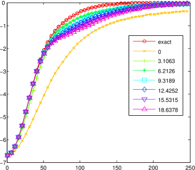
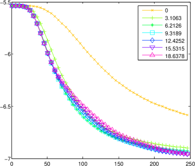
Figure 1: The experimental setting is the same as in fig(2). (a) Plotted is the value of the exact log likelihood based on gradient ascent of the ranking objective for different $\alpha$ values. In this case $\log(C-1)=6.2126$ is the suggested optimal setting. We also plot the log likelihood for the exact gradient. (b) The bias, represented as the log mean absolute difference between the class probability predictions based on the current parameters learned and the class predictions for the true underlying model (see also section(4).

3.3.2 Negative Sampling

A similar approach to ranking is to maximise $\log\sigma(\mathbf{w}_{c}^{\textsf{T}}\mathbf{x})$ whilst minimising $\log\sigma(\mathbf{w}_{d}^{\textsf{T}}\mathbf{x})$, for a randomly chosen subset of negative classes $d\neq c$. This is motivated in [10] as an approximation of the NCE method and has the objective

$$\log\sigma\left({\mathbf{w}_{c}^{\textsf{T}}\mathbf{x}}\right)+\sum_{d}\log\left({1-\sigma\left({\mathbf{w}_{d}^{\textsf{T}}\mathbf{x}}\right)}\right)$$ (43)

This has gradient wrt $\mathbf{w}_{a}$ given by

$$\left({\left({1-\sigma\left({\mathbf{w}_{c}^{\textsf{T}}\mathbf{x}}\right)}\right)\delta_{ac}-\sum_{d}\sigma\left({\mathbf{w}_{d}^{\textsf{T}}\mathbf{x}}\right)\delta_{ad}}\right)\mathbf{x}$$ (44)

For ease of comparison, we scale this number of negative terms to have a similar effect to the positive term, giving for a member $m$ of the minibatch

$$\gamma_{m}^{-}(c)\equiv\frac{1}{|\mathcal{C}^{\prime}|-1}\sum_{d\in\mathcal{C}^{\prime}\backslash c}\left({\left({1-\sigma\left({\mathbf{w}_{c_{m}}^{\textsf{T}}\mathbf{x}_{m}}\right)}\right)\delta_{c,c_{m}}-\sigma\left({\mathbf{w}_{d}^{\textsf{T}}\mathbf{x}_{m}}\right)\delta_{c,d}}\right)$$ (45)

The negative sampling approach approximation to $\gamma_{m}(c)$ therefore has the correct sign and lies between $-1$ and $1$. As pointed out in [10] this objective will not, in general, have its optimum at the same point as the log likelihood. For the simple softmax regression model, we found that this approach does not yield practically useful results and as such is not considered further. The main motivation for the method is that it is a fast procedure which empirically results in useful parameters when applied in a more complex wordvec setting [10].

3.4 BlackOut

The recently introduced BlackOut [9] is a discriminative approach based on an approximation to the true discrimination probability. This forms the approximation

$$\tilde{p}(c|x,\theta)=\frac{q_{c}u_{\theta}(c,x)}{q_{c}u_{\theta}(c,x)+\sum_{d\in\mathcal{N}}q_{d}u_{\theta}(d,x)}$$ (46)

Here $q_{c}=1/Q(c)$ where $Q(c)$ is a distribution over all classes $1,\ldots,C$. The ratio $q_{c}=1/Q(c)$ is inspired by Importance sampling. Training is based on maximising the discriminative objective

$$\log\tilde{p}(c_{m}|x_{m},\theta)+\sum_{d\in\mathcal{N}}\log\left({1-\tilde{p}(d|x_{m},\theta)}\right)$$ (47)

where $c_{m}$ is the correct class for input $x_{m}$ and $\mathcal{N}_{c}$ is a set of ‘negative’ classes for $c_{m}$. The objective is summed over all points in the minibatch. BlackOut shares similarities with NCE but avoids the difficulty of the unknown normalisation constant. For the IS distribution $Q(c)$ the authors propose to use $Q(c)\propto f(c)^{\alpha}$ where $f(c)$ is the empirically observed class distribution $f(c)\propto\sum_{n}\mathbb{I}\left[{c_{n}=c}\right]$ and $0\leq\alpha<1$ is found by validation. BlackOut shares similarities with our normalisation approach. However, the training objective is different – BlackOut uses a discriminative criterion rather than the likelihood. Whilst the optimum of the BlackOut objective can be shown to match the log likelihood objective (in the limit of a large number of samples) it is unclear why the BlackOut objective might be preferable to a direct log likelihood approximation.

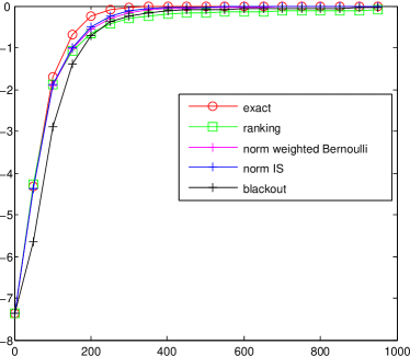
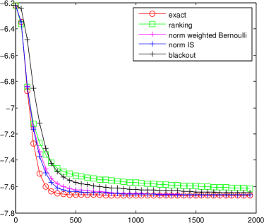
Figure 2: (a) Plotted is the value of the exact log likelihood (y-axis) against iteration number (x-axis) for a set of $N=2000$ datapoints, each $D=100$ dimensional. There are $C=1000$ classes and the training data was generated from the model to make a realisable problem. We compute the exact gradient for each minibatch of $|\mathcal{M}|=50$ datapoints and also compute the comparative and normalisation approximations for the minibatch. In all approximations, $K=20$ additional ‘negative’ classes were randomly sampled in addition to the classes in each minibatch. All approximations used roughly $1050$ calculations of the form $\exp(\mathbf{w}^{\textsf{T}}\mathbf{x})$ per minibatch, compared to 50,000 calculations for the exact approach, leading to a roughly 50 fold decrease in computation cost. The plot shows gradient ascent with momentum $0.99$. Learning rates for the exact, and normalisation approximations were all set the same; the BlackOut and Ranking learning rates were set to the largest values that ensured convergence. The Noise Contrastive Estimation and Negative Sampling approaches are not shown since here $z_{m}=1$ results in very poor performance. (b) The log mean absolute difference between the current parameters learned based on the exact gradient update and the parameters learned by each approximation. This indicates the bias in learning the parameters. All approaches were initialised with the same initial parameters, so that at the first iteration there is no difference between the parameters.

4 Experiment

We consider the simple softmax regression model $u(c,x)=\exp(\mathbf{w}_{c}^{\textsf{T}}\mathbf{x})$. The exact log-likelihood in this case is concave, as are our sampling approximations. This is useful since the convexity of the objective means that the results do not depend on the difficulty of optimisation and focus on the quality of the objective in terms of mimicking the true log likelihood. To estimate the performance of the trained models, we note that the model is invariant up to $\mathbf{w}_{c}^{\textsf{T}}\mathbf{x}+a(\mathbf{x})$ for any $a(\mathbf{x})$. This invariance means that directly comparing parameters from trained models is problematic. For this reason, we estimate bias by looking at the predictive performance of a model $p_{\theta}(c|x)$ compared to the predictive performance of the true model $p_{\theta_{0}}(c|x)$. In particular we measure the log mean absolute difference in class probability prediction for the inputs in the training set. Neither Noise Contrastive Estimation (with $z_{m}=1$) nor Negative Sampling are given in the results since these approaches perform significantly worse than the other approaches. 

In fig(2) we show results for a simple experiment that compares the exact minibatch gradient compared to our normalisation approximations, ranking and BlackOut. This experiment shows that whilst all methods work reasonably well, the normalisation approximations result in the most rapidly convergent in terms of bias minimisation. The empirical class frequency $Q(c)=f(c)$ was used to form the Importance sampling distribution and $K=20$ results in $b(c)=f(c)^{0.54}$ for the Bernoulli probabilities. There appears little difference between the Bernoulli and Importance sampling approaches which is somewhat unexpected. It is possible that the theoretical benefit of the Bernoulli sampling in terms of a lower variance estimator is dwarfed by the stochasticity induced by the minibatch sampling process.

5 Discussion

In contrast to recently introduced alternative approaches, a simple approximation of the the standard maximum likelihood objective provides an easily implementable and competitive method for fast large-class classification.  

An insight from our normalisation approximation is that it relates to the ranking objective and indeed justifies why an offset term can significantly improve the ranking objective.  

We also experimented with a deterministic approximations based on based on variations of the result

$$Z =\sum_{i=1}^{C}\exp{v_{\theta}(i,x)}=\sum_{i=1}^{C}\exp\left({\mathbb{E}_{s_{i}}\left({\frac{s_{i}v_{\theta}(i,x)}{b_{i}}}\right)}\right)\leq C+\mathbb{E}_{\mathbf{s}}\left({\sum_{i=1}^{C}{s_{i}\left({\exp\left({\frac{v_{\theta}(i,x)}{b_{i}}}\right)-1}\right)}}\right)$$ (48)

where $s_{i}$ are Bernoulli random variables and $b_{i}=p(s_{i}=1)$. However, these approaches were less successful in this context than the simple sampling approximations.

References

- [1] Y. Bengio and J-S. Senécal. Quick training of probabilistic neural nets by sampling. AISTATS, 9, 2003.
- [2] Y. Bengio and J-S. Senécal. Adaptive Importance Sampling to Accelerate Training of a Neural Probabilistic Language Model. IEEE Transactions on Neural Networks, 19(4):713–722, 2008.
- [3] T. E. Booth. Unbiased Monte Carlo Estimation of the Reciprocal of an Integral. Nuclear Science and Engineering, 156(3):403–407, 2007.
- [4] R. Collobert and J. Weston. A unified architecture for natural language processing: Deep neural networks with multitask learning. In Proceedings of the 25th International Conference on Machine Learning, ICML ’08, pages 160–167, New York, NY, USA, 2008. ACM.
- [5] C. J. Geyer. On the convergence of Monte Carlo maximum likelihood calculations. Journal of the Royal Statistical Society, Series B (Methodological), 56(1):261––274, 1994.
- [6] M. Gutmann and A. Hyvärinen. Noise-contrastive estimation: A new estimation principle for unnormalized statistical models. International Conference on Artificial Intelligence and Statistics, pages 1–8, 2010.
- [7] M. U. Gutmann and A. Hyvärinen. Noise-contrastive estimation of unnormalized statistical models, with applications to natural image statistics. The Journal of Machine Learning Research, 13(1):307–361, 2012.
- [8] S. Jean, K. Cho, R. Memisevic, and Y. Bengio. On Using Very Large Target Vocabulary for Neural Machine Translation. Proceedings of the 53rd Annual Meeting of the Association for Computational Linguistics and the 7th International Joint Conference on Natural Language Processing (Volume 1: Long Papers), pages 1–10, 2015.
- [9] S. Ji, S. V. N. Vishwanathan, N. Satish, M. J. Anderson, and P. Dubey. BlackOut: Speeding up Recurrent Neural Network Language Models With Very Large Vocabularies. ICLR, pages 1–12, 2016.
- [10] T. Mikolov, I. Sutskever, K. Chen, G. S Corrado, and J. Dean. Distributed representations of words and phrases and their compositionality. In C. J. C. Burges, L. Bottou, M. Welling, Z. Ghahramani, and K. Q. Weinberger, editors, Advances in Neural Information Processing Systems 26, pages 3111–3119. Curran Associates, Inc., 2013.
- [11] A. Mnih and K. Kavukcuoglu. Learning word embeddings efficiently with noise-contrastive estimation. Neural Information Processing Systems, pages 1–9, 2013.
- [12] A. Mnih and Y. W. Teh. A Fast and Simple Algorithm for Training Neural Probabilistic Language Models. Proceedings of the 29th International Conference on Machine Learning (ICML’12), pages 1751–1758, 2012.
- [13] F. Morin and Y. Bengio. Hierarchical probabilistic neural network language model. In Proceedings of the international workshop on artificial intelligence and statistics, pages 246––252. 2005.