Disordered double Weyl node: Comparison of transport and density-of-states calculations

Abstract

Double Weyl nodes are topologically protected band crossing points which carry chiral charge $\pm 2$. They are stabilized by $C_{4}$ point group symmetry and are predicted to occur in $\mathrm{SrSi_{2}}$ or $\mathrm{HgCr_{2}Se_{4}}$. We study their stability and physical properties in the presence of a disorder potential. We investigate the density of states and the quantum transport properties at the nodal point. We find that, in contrast to their counterparts with unit chiral charge, double Weyl nodes are unstable to any finite amount of disorder and give rise to a diffusive phase, in agreement with predictions of Goswami and Nevidomskyy [Phys. Rev. B 92, 214504 (2015)] and Bera, Sau, and Roy [Phys. Rev. B 93, 201302(R) (2016)]. However, for finite system sizes a crossover between pseudodiffusive and diffusive quantum transport can be observed.

I Introduction

Topological metals and semimetals are among the driving themes in contemporary condensed matter physics. Their most prominent three-dimensional realizations are Weyl (semi)metals, which have recently been experimentally confirmed in a number of different material systems Bernevig (2015); Xu et al. (2015a); Lv et al. (2015); Xu et al. (2015b); Borisenko et al. (2015); Liu et al. (2015). Pioneering experimental studies used spectroscopic measurements to study surface Fermi arcs and characteristic Weyl node bulk dispersions. Recently, also (magneto-)transport properties received growing interest in experiment Zhang et al. (2016, 2015); Shekhar et al. (2015).

While sample quality matures continuously, more controlled engineering of the chemical potential comes into reach Ruan et al. (2016a, b). Weyl nodes with chemical potential $\mu$ sufficiently close to the nodal point ($\mu=0$) are predicted to show unusual transport characteristics for sample length $L\lesssim\hbar v/\mu$, with $v$ the Fermi velocity Baireuther et al. (2014); Sbierski et al. (2014). Without disorder, the conductance scales with system size as $G\propto W^{2}/L^{2}$, where $W$ is the sample width. The inclusion of weak disorder is irrelevant in the renormalization-group (RG) sense Fradkin (1986); Goswami and Chakravarty (2011); Kobayashi et al. (2014); Ominato and Koshino (2014); Syzranov et al. (2015a, b) and consequently does not change the size dependence of the conductance. This so-called “pseudoballistic” regime is further characterized by an unusual Fano factor (the ratio of shot-noise power and average current) $F\approx 0.57$ Baireuther et al. (2014); Sbierski et al. (2014). Only if disorder increases above a critical strength, the conductivity and density of states at the nodal point attains a non-zero value and transport becomes diffusive, $G\propto W^{2}/L$ and $F=1/3$.

The simple Weyl node (SWN) band structure discussed above carries a topological charge of $\pm 1$. Beyond the SWN, the existence of topological band touching points with higher topological charge is tied to the presence of point-group symmetries Fang et al. (2012). In this paper, we consider double Weyl nodes (DWN) with chiral charge of magnitude two, stabilized by $C_{4}$ rotation symmetry. The Hamiltonian reads

$$H=\hbar v[\sigma_{x}\eta_{x}\,(k_{x}^{2}-k_{y}^{2})/2+\sigma_{y}\eta_{y}\,k_{x}k_{y}+k_{z}\sigma_{z}],$$ (1)

with $\eta_{x,y}$ internal length scales. The fourfold rotational symmetry around the $z$-axis is realized as $H\!\left(k_{x},k_{y},k_{z}\right)=\sigma_{z}H\left(k_{y},-k_{x},k_{z}\right)\sigma_{z}$. Time-reversal symmetry is present, $\sigma_{x}H^{*}\left(-\mathbf{k}\right)\sigma_{x}=H\left(\mathbf{k}\right)$ with the time reversal operator $T=\sigma_{x}K$ squaring to $+1$. To simplify the subsequent analysis, we specialize to the case $\eta_{x}=\eta_{y}\equiv\eta$ where the discrete rotation symmetry is extended to a continuous rotation symmetry $C_{\infty}$, in cylindrical coordinates $H\left(k_{\perp},\phi,k_{z}\right)=e^{-i\theta\sigma_{z}}H\left(k_{\perp},\phi-\theta,k_{z}\right)e^{i\theta\sigma_{z}}$. The corresponding energy dispersion $\varepsilon_{\pm}^{2}/(\hbar v)^{2}=(k_{\perp}^{2}\eta/2)^{2}+k_{z}^{2}$ is quadratic in the momentum $\mathbf{k}_{\perp}=(k_{x},k_{y})$ transverse to the rotation axis and linear in $k_{z}$, see Fig. 1(a). A photonic crystal realization of DWNs is reported in Ref. Chen et al. (2015) and fermionic candidate materials have been identified from first-principle calculations, such as $\mathrm{HgCr_{2}Se_{4}}$Xu et al. (2011) or $\mathrm{SrSi_{2}}$Huang et al. (2016). The latter material might be experimentally more feasible since no magnetic ordering is required. An interesting proposal to detect the monopole charge in electronic Weyl materials using transport measurements has recently been formulated in Ref. Dai et al., 2016.

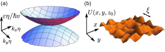
Figure 1: (a) Dispersion for DWN Hamiltonian $H$ with $\eta_{x,y}=\eta$ in Eq. (1) at $k_{z}=0$. (b) The potential disorder profile is characterized by its Gaussian correlations decaying on a length scale $\xi$, here a slice at $z=z_{0}$ is shown.

In view of the requirement of point-group symmetries, the stability of a DWN to disorder, which typically breaks such symmetry [see Fig. 1(b)], is a relevant question. Several groups have addressed this question theoretically, with partially diverging results. Using a simplified version of the self-consistent Born approximation, Goswami and Nevidomskyy Goswami and Nevidomskyy (2015) argued that the DWN is unstable to disorder, and that inclusion of even a small amount of disorder drives the system to a diffusive phase with zero-energy scattering rate $\hbar/\tau\sim e^{-A/K}$, where $K$ is a dimensionless measure of the disorder strength and $A$ a material-dependent parameter. The same conclusion was drawn by Bera, Sau and Roy Bera et al. (2016), based both on an RG analysis [which found disorder a marginally relevant perturbation to Eq. (1)] and a numerical calculation of the density of states at zero energy, which was claimed to be compatible with the exponential form proposed above.

Recently, Shapourian and Hughes Shapourian and Hughes (2016) revisited the same problem, conducting a finite-size scaling analysis of the decay length in the $z$ direction using a transfer-matrix method. Their data indicates the presence of a critical point at a finite disorder strength (but below the Anderson transition), leading them to conclude the stability of the DWN phase against weak disorder. A possible scenario for such an observation would be the splitting of the DWN into two equally charged SWNs under the influence of disorder, where the latter individually would indeed feature a critical point. This interesting scenario and the apparent contradiction between results in the literature motivated us to revisit the problem of a disordered DWN.

We first investigate the density of states using the Kernel Polynomial method and the self-consistent Born approximation (Sec. II). We discuss the shortcomings of either method and move on to a scattering matrix-based transport calculation, much better suited to study the physics right at the nodal point (Sec. III). These combined numerical efforts allow us to put forward the following interpretation: In the presence of any finite amount of disorder, the clean DWN fixed point is unstable and gives rise to a diffusive phase. We find no evidence in support of a critical point at finite disorder strength and, accordingly, of the DWN splitting scenario. However, due to exponentially small scattering rate, a crossover behavior can be observed in the quantum transport properties of weakly disordered mesoscopic samples.

II Density of states

II.1 Kernel-Polynomial Method

We start by calculating the density of states in a disordered DWN which we regularize on a cubic lattice

$$H_{\mathrm{L}}(\mathbf{k}) \!= \!\varepsilon_{0}\frac{\eta}{a}\left[\sigma_{x}(\cos ak_{x}-\cos ak_{y})+\sigma_{y}\sin ak_{x}\sin ak_{y}\right]$$ (2)

$$-\varepsilon_{0}\sigma_{z}\cos ak_{z}$$

where $\varepsilon_{0}=\hbar v/a$ and $a$ is the lattice constant. The effective low energy approximation of $H_{\mathrm{L}}$ around $\varepsilon=0$ consists of four DWNs centered at $k_{z}=\pm\frac{\pi}{2a}$ and $(k_{x},k_{y})=(0,0)$ or $(\frac{\pi}{a},\frac{\pi}{a})$ with minimal distance $\Delta k=\pi/a$. We include a Gaussian disorder potential $U(\mathbf{r})$ characterized by zero mean and real space correlations given by

$$\left\langle U(\mathbf{r})U(\mathbf{r}^{\prime})\right\rangle_{\rm dis}=\frac{K\left(\hbar v\right)^{2}}{\sqrt{2\pi}^{3}\xi^{2}}e^{-|\mathbf{r}-\mathbf{r}^{\prime}|^{2}/2\xi^{2}},$$ (3)

where $\xi$ is the correlation length and $K$ the dimensionless disorder strength. In the following, we use $\xi=\eta/2$ but different choices do not qualitatively change our conclusions. To smoothly represent $U(\mathbf{r})$ on the lattice scale, we take $\xi=2.9a$ which suppresses the inter-node scattering rate by a factor $e^{-(\Delta k)^{2}\xi^{2}/2}<10^{-18}$ compared to the intra-node rate, so single node physics (i.e. $H+U$) is realized to a very good approximation.

We numerically calculate the density of states of $H_{\mathrm{L}}+U(\mathbf{r})$ using the Kernel Polynomial method (KPM) (see Ref. Weisse et al. (2006) for a description of the method). The resulting density of states normalized to a single DWN is shown as solid lines in Fig. 2(a). Further simulation parameters are given in the figure caption. The analytical result for an infinite clean system,

$$\nu_{0}(\varepsilon)=\frac{\varepsilon}{4\pi\left(\hbar v\right)^{2}\eta},$$ (4)

is shown as a dotted line in Fig. 2 and compares well with the $K=0$ KPM results except at $\varepsilon=0$. At the nodal point, the KPM method has intrinsic difficulties to simulate the vanishing (or very small) density of states, which is due to the finite expansion order of $\nu(\varepsilon)$ in Chebyshev polynomials and the discrete nature of eigenstates in a finite tight-binding model. In Fig. 2(b), we plot $\nu(\varepsilon=0)$ vs. $K$. Our findings are in qualitative agreement with similar numerical results in Ref. Bera et al., 2016: The presence of disorder scattering fills the dip in the density of states for any finite disorder strength.

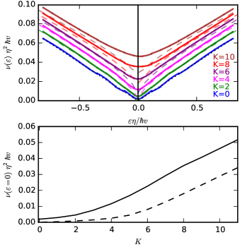
Figure 2: Density of states $\nu$ as a function of energy $\varepsilon$ (top) and at the nodal point $\varepsilon=0$ (bottom) normalized to a single DWN as computed from the Kernel polynomial method (KPM) applied to the lattice Hamiltonian $H_{\mathrm{L}}$ (solid lines). The results of the self-consistent Born approximation based on $H$ (dashed lines) are in good agreement with the KPM data except in the vicinity of the nodal point and for large disorder strengths $K>6$. We take the disorder correlation length $\xi=\eta/2$. The system size of the tight-binding model underlying the KPM calculation is $L_{x,y}=100a$, $L_{z}=260a$ and we apply periodic boundary conditions. The expansion order in Chebyshev Polynomials $N$ is taken in between 1000 and 6000 depending on the energy $\varepsilon$ so that $\nu$ is minimized but oscillations due to the underlying discrete Eigenenergies of the finite system are sufficiently smoothed out. An average over 10 disorder realizations is taken and 20 random vectors were used to calculate the trace in the KPM.

II.2 Self-consistent Born approximation

A frequently employed analytical approach to disordered electronic systems is the self-consistent Born approximation (SCBA). Although a simplified SCBA calculation has been performed in Ref. Goswami and Nevidomskyy, 2015, in the following we compute the SCBA self-energy for $H+U$ and the associated density of states without any further approximations. The results are shown as dashed lines in Fig. 2, comparison to the KPM results confirm that SCBA is accurate only at large energies $\varepsilon$ and weak disorder values, when $\varepsilon\tau\gg\hbar$ with $\tau$ being the quasiparticle scattering time.

We start from Hamiltonian $H$ with $\eta_{x}=\eta_{y}\equiv\eta$ and seek to describe the disorder averaged retarded Green function $\left\langle G^{R}\right\rangle_{\rm dis}=1/(\varepsilon-H-\Sigma^{R})$ in terms of a translationally invariant self energy term $\Sigma^{R}$ that fulfills the SCBA equation

$$\Sigma^{R}(\mathbf{k})=\int\frac{d\mathbf{k}^{\prime}}{(2\pi)^{3}}\left\langle G^{R}(\mathbf{k}^{\prime})\right\rangle_{\rm dis}\left|U(\mathbf{k}^{\prime}-\mathbf{k})\right|^{2}$$ (5)

where $\left|U(\mathbf{k}^{\prime}-\mathbf{k})\right|^{2}$ is the Fourier transform of the disorder correlator in Eq. (3). Since a disorder average restores the $C_{\infty}$-symmetry of the system around the $k_{z}$ axis, the projection of $\Sigma^{R}(k,\phi,k_{z})$ to the $\sigma_{x}-\sigma_{y}$ plane in Pauli-matrix space should point into $\phi$ direction, the angle between this plane and the $\sigma_{z}$ projection of $\Sigma^{R}(k,\phi,k_{z})$ is not dictated by symmetry and can be different from the angle in $H\left(k,\phi,k_{z}\right)$. With these considerations, a natural ansatz for the self energy is

$$\Sigma^{R}(k,\phi,k_{z})/\hbar v \!= m(k,k_{z})\!\left(\cos\left[2\phi\right]\sigma_{x}+\sin\left[2\phi\right]\sigma_{y}\right)$$ (6)

$$+\sigma_{z}m_{z}\left(k,k_{z}\right)-im_{0}\left(k,k_{z}\right)$$

with $m$, $m_{z}$ and $m_{0}$ complex and $Re[m_{0}]>0$. At $\varepsilon=0$, in order to avoid an unphysical spontaneous generation of a chemical potential from disorder with $\left\langle U(\mathbf{r}))\right\rangle_{\rm dis}=0$, $m_{0}$ has to be chosen purely real which enforces also $m$ and $m_{z}$ to be real quantities. The resulting self-consistency equations for $m$, $m_{z}$ and $m_{0}$ are given in the appendix and can be solved numerically by iteration. The density of states follows from

$$\nu\left(\varepsilon\right)=-\frac{1}{\pi}\mathrm{Im}\int\frac{d\mathbf{k}}{(2\pi)^{3}}\mathrm{Tr}\left\langle G^{R}(\mathbf{k})\right\rangle_{\rm dis}.$$ (7)

Results of this calculation are shown as dashed lines in Fig. 2 for various representative disorder strengths $K$.

II.3 Discussion

The SCBA calculation in Sec. II can be simplified by taking the disorder correlation length to zero and choosing a finite (half-)bandwidth $\Lambda\gg\hbar v/\eta$. Then we could define $K$ such that $\left|U(\mathbf{k}^{\prime}-\mathbf{k})\right|^{2}=K\Lambda^{2}\eta^{3}$ and insert this in Eq. (5) at $\varepsilon=0$, where $\Sigma^{R}\equiv-i\Gamma$ becomes independent of $\mathbf{k}$. Transforming to an energy integral and using the density of states (4) along with the assumption $\Gamma\ll\Lambda$, one finds

$$\Gamma=\Lambda e^{-A/K}$$ (8)

with $A=2\pi\left(\hbar v/\Lambda\eta\right)^{2}$. This was first observed by Goswami and Nevidomskyy in Ref. Goswami and Nevidomskyy, 2015 and states that any finite disorder strength gives rise to a finite lifetime $1/\Gamma$ of quasiparticles and a finite density of states $\nu(\varepsilon=0)\propto\Gamma$ at the nodal point. Our SCBA analysis which takes into account a more realistic disorder model and infinite bandwidth confirms the simplified result in Eq. (8) qualitatively, see dashed line in Fig. 2 bottom panel.

However, it is well known that the SCBA is not reliable around gapless points, where the smallness of the parameter $k_{F}l$ spoils the suppression of crossed diagram contributions to the self energy (see, e.g. Ref. Sbierski et al. (2014) for a discussion in the context of simple Weyl nodes). Indeed, comparing the non-perturbative KPM results for $\nu(\varepsilon)$ to the SCBA in Fig. 2, good agreement is achieved away from the nodal point only. At the nodal point, it is difficult to judge the qualitative validity of Eq. (8) based on the KPM results. The reason is that, for the latter method, finite size and smoothing effects tend to overestimate $\nu(\varepsilon=0)$. (For example, the KPM method returns a finite value of $\nu(\varepsilon=0)$ even for $K=0$, see Fig. 2, bottom panel.) In summary, neither numerical nor analytical calculations of the density of states as presented above are conclusive in gauging the qualitative validity of Eq. (8) against the alternative scenario of a finite critical disorder strenght below which the bulk density of states vanishes. In this situation, we switch to a quantum transport framework which is ideally suited to study the disordered DWN at the nodal point.

III Quantum transport

III.1 Clean case

We start this section by calculating the conductance and shot noise power of a clean mesoscopic DWN sample of length $L$ and width $W$ coupled to ideal leads, building on earlier work by Tworzydlo et al. on two-dimensional Dirac nodes Tworzydlo et al. (2006). We choose the transport direction as the $z$ direction and place the chemical potential at the nodal point. We model the leads as highly doped DWNs, $H_{\mathrm{lead}}=H+V$ with $V\rightarrow\infty$. By matching wavefunctions at the sample-lead interfaces we calculate the transmission amplitudes $t_{0}(\mathbf{k}_{\perp})$ and $t_{0}^{\prime}(\mathbf{k}_{\perp})$ and reflection amplitudes $r_{0}(\mathbf{k}_{\perp})$ and $r_{0}^{\prime}(\mathbf{k}_{\perp})$, where the primed (unprimed) amplitudes refer to electrons incident from the positive (negative) $z$ direction,

$$t_{0}=t_{0}^{\prime} = 1/\cosh(\eta Lk_{\perp}^{2}/2),$$

$$r_{0}=-r_{0}^{\prime*} = ie^{-2i\varphi}\tanh(\eta Lk_{\perp}^{2}/2),$$ (9)

$\mathbf{k}_{\perp}=(k_{x},k_{y})$ the transverse component of the wavevector, and $\varphi=\arctan(k_{y}/k_{x})$ is the azimuthal angle of incidence. The associated basis spinors for propagating states in the lead are $(0,1)^{\mathrm{T}}$ and $(1,0)^{\mathrm{T}}$ for left- and right-moving modes, respectively. From the transmission amplitude $t_{0}(\mathbf{k}_{\perp})$ we compute the clean-limit conductance and Fano factor as $G_{0}=\frac{e^{2}}{h}\mathrm{tr}[t_{0}^{\dagger}t_{0}]$ and $F_{0}=\mathrm{tr}[t_{0}t_{0}^{\dagger}(1-t_{0}t_{0}^{\dagger})]/\mathrm{tr}[t_{0}t_{0}^{\dagger}]$ Nazarov and Blanter (2009). Modes with $k_{\perp}\gg(L\eta)^{-1/2}\equiv k_{\perp}^{\star}\left(L\right)$ are strongly suppressed in transmission and the spacing of the quantized transversal wave vectors in a finite sample is $\Delta k_{\perp}=2\pi/W$. If $\Delta k_{\perp}\ll k_{\perp}^{*}$, we can compute conductance and Fano factor analytically by replacing the sum over discrete modes $\mathbf{k}_{\perp}$ by an integral and find

$$G_{0}\left(W,L\right) = \frac{e^{2}}{h}\frac{1}{2\pi\eta}\frac{W^{2}}{L},$$ (10)

$$F_{0}\left(W,L\right) = 1/3,$$ (11)

which resembles transport in a diffusive conductor with conductivity $\sigma_{0}=e^{2}/(2\pi h\eta)$. Thus, the clean DWN has pseudodiffusive transport characteristics — similar to Dirac electrons in two dimensions Tworzydlo et al. (2006).

III.2 Disordered case

We extend the scattering matrix approach to include a Gaussian disorder potential $U(\mathbf{r})$ with correlations as in Eq. (3) and $\xi=\eta/2$ like in the density of states calculation. We compute the transmission matrix of the disordered DWN $H+U(\mathbf{r})$ by concatenating the reflection and transmission amplitudes of a thin slice of DWN without disorder, see Eq. (9), with reflection and transmission matrices of a thin slice with disorder, which can be calculated using the first-order Born approximation, and repeating this procedure for many slices. We apply periodic or antiperiodic boundary conditions in the $x$ and $y$ directions, cutting off the number of transverse modes to keep the dimensions of the transmission and reflection matrices finite. We take the mode cutoff large enough and the slice length thin enough so that the results do not depend on either, and we take $\Delta k_{\perp}/k_{\perp}^{*}$ small enough that the results do not depend on the choice of the boundary conditions. A similar method has been previously applied to study disordered Dirac materials in two Bardarson et al. (2007); Adam et al. (2009) and in three dimensions Sbierski et al. (2015, 2014), and we refer to those references for more details on the numerical method.

Figure 3 shows our results for the resistance $R=1/\langle{G}\rangle_{\mathrm{dis}}$ as a function of sample length $L$, where $\langle{...}\rangle_{\mathrm{dis}}$ denotes an average over 60 disorder realizations as well as the two choices for the boundary conditions, to further suppress statistical uncertainty. Compared to the clean pseudo-resistance $R_{0}=L/(\sigma_{0}W^{2})$, the resistance of the disordered samples is slightly decreased by up to about 10 percent, see top panel. The difference $\Delta R=R_{0}-R$ is shown in the bottom panel. For the smallest disorder strength considered, $K=1$, $\Delta R$ scales linearly with $L$ for the system lengths considered, for intermediate $K=2,4,6$, $\Delta R$ is not a linear function of $L$ but instead has an “S”-like dependence, which prevents any meaningful assignment of a (change of the) bulk resistivity. The resistance at the largest system size $R(L_{\rm max}=72\eta)$, shows a non-monotonous behavior with increasing disorder strength. For larger $K=8,10,14$, the $\Delta R$ traces are purely convex and tend to be linear for large $L$. We have also investigated the Fano factor which stays around $F=1/3$ (not shown) for all values of $K$.

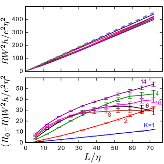
Figure 3: Resistance for disordered DWN for disorder strengths $K=1$, $2$, $4$, $6$, $8$, $10$, and $14$ and disorder correlation length $\xi=\eta/2$. Results are averaged over periodic and antiperiodic transverse boundary conditions and over 60 disorder realizations per boundary condition. The dashed line indicates the clean-limit pseudodiffusive result of Eq. (10). We chose $W=72\eta$, and keep transverse modes with $|k_{x,y}|<2\pi M/W$ with $M=34$.

III.3 Discussion

A finite lifetime $1/\Gamma$ implies diffusive transport with resistance scaling $R\propto L$. While this is (approximately) observed in our transport simulations for $K>0$, see Fig. 3 top panel, the difficulty lies in the discrimination to transport behavior associated to the clean fixed point $K=0$: Being pseudodiffusive, the same resistance scaling holds, albeit for the very different reason of evanescent wave physics and not due to scattering between transport channels as in diffusive transport. To discriminate between the pseudodiffusive and diffusive regimes, in Fig. 4 (top) we show the probability $P_{\rm t}(L)$ that an electron is transmitted in the same transverse mode as it enters — for which we take the mode with $\mathbf{k}_{\perp}=0$ —, conditional on the probability that it is transmitted,

$$P_{\rm t}(L)=\frac{|t(0,0)|^{2}}{\sum_{\mathbf{k}_{\perp}}|t(\mathbf{k}_{\perp},0)|^{2}},$$ (12)

where $t(\mathbf{k}_{\perp}^{\rm{out}},\mathbf{k}_{\perp}^{\rm{in}})$ is the transmission amplitude of the disordered system at length $L$, $\mathbf{k}_{\perp}^{\rm{out}}$ and $\mathbf{k}_{\perp}^{\rm{in}}$ referring to the incoming and outgoing transverse modes.

The conditional probability $P_{\rm{t}}$ is an indicator of the transition between the pseudodiffusive and diffusive regimes: At the pseudodiffusive fixed point $K=0$ one has $P_{\rm{t}}(L)=1$, as translational translational invariance ensures that $t(\mathbf{k}_{\perp}^{\rm out},\mathbf{k}_{\perp}^{\rm in})$ is diagonal in the transversal mode indices $\mathbf{k}_{\perp}^{\rm in}$ and $\mathbf{k}_{\perp}^{\rm out}$, see (9). In contrast, diffusive transport is characterized by scattering between transverse modes. For sufficiently long diffusive samples with many transverse modes one therefore expects $P_{\rm{t}}(L)\to 1/N_{\perp}$, where $N_{\perp}$ is the total number of transverse modes. For finite-length samples $P_{\rm{t}}(L)$ is expected to approach this asymptotic value from above, starting from $P_{\rm{t}}(0)=1$ in the limit of zero sample length. For the disordered DWN system our data in Fig. 4 (top) indeed indicates a monotonous decrease of $P_{\rm{t}}(L)$ with $L$ and a saturation at large $L$ for disorder strengths $K>4$. Although no saturation could be observed for weaker disorder strength at the system sizes we could access in our numerical calculations, we found no sign that $P_{\rm{t}}(L)$ behaves differently for $K<4$, consistent with with a flow to a diffusive fixed point even for weak disorder. On the other hand, if weak disorder is an irrelevant perturbation (as it is in the case of a single Weyl node) and the pseudodiffusive fixed point would be stable, we would expect that an initial decrease of $P_{\rm{t}}(L)$ with $L$ is compensated by increase of $P_{\rm{t}}(L)$ at larger lenghts, a behavior that we confirmed for the weakly disordered SWN (data not shown).

As long as $P_{\rm t}\gg 1/N_{\rm t}$, where $N_{\rm t}\sim hG/e^{2}\sum_{\mathbf{k}_{\perp}}|t(\mathbf{k}_{\perp},0)|^{2}$ is the (effective) number of transverse modes participating in the transmission, a condition that is met for the entire parameter range we consider, we expect that $P_{\rm t}(L)$ has the functional form

$$P_{\rm t}(L)=e^{-(L-L_{c})/L^{\star}},$$ (13)

where the characteristic length scale $L^{\star}$ can be identified with the mean free path and $L_{c}$ a length scale that accounts for transient effects at the sample-lead boundary, leading to a quick initial decrease of $P_{\rm t}$ for short lengths, in particular visible for $K\lesssim 4$. The lower panel of Fig. 4 shows fits of $L^{\star}$ based on the large-$L$ asymptotics of $P_{\rm t}(L)$. The $K$ dependence of $L^{\star}$ is consistent with the expectation based on Eq. (8), $L^{\star}\sim\hbar v/\Gamma\sim\hbar v/\Lambda e^{A/K}$. We disregard the data points at $K=1$ and $K=2$, for which no reliable asymptotic large-$L$ fit could be made.

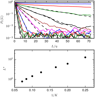
Figure 4: Top: Conditional same-mode transmission probability $P_{\rm t}(L)$ for disorder strengths $K=0,1$, $2$, $3$, $4$, $5$, $6$, $8$, $10$, $12$, and $14$ (top to bottom curve). The dashed lines denote fits to the form $\exp(-(L-L_{c})/L^{\star})$. Bottom: Mean free path $L^{\star}$, obtained from the fits to $P_{\rm t}(L)$, versus $1/K$.

The curves for the difference $\Delta R(L)$ of the resistances in the clean and disordered cases in Fig. 3 can be understood in terms of a crossover from pseudodiffusive to diffusive transport as well. The length scale $L^{\star}(K)$ roughly coincides with the length scale where the second derivative of the resistance vs. sample length curve vanishes.

For the weakest disorder strength we consider the maximum sample length $L_{\rm max}$ is still much smaller than the characteristic length $L^{*}$ of the pseudodiffusive-to-diffusive crossover. For this disorder strength, pseudodiffusive behavior prevails for all system sizes we consider, albeit with a resistance that is slighlty smaller than $R_{0}$. A decrease of the resistivity has also been observed as a finite-size effect for a SWN at weak disorder strengths Sbierski et al. (2014). A systematic decrease of the resistivity could in principle arise as a consequence of a disorder-induced renormalization of the parameters $v$ and $\eta$ in the Hamiltonian (1). For a bulk system, the renormalized parameters $v_{\rm eff}$ and $\eta_{\rm eff}$ can be calculated in the Born approximation, which yields an increased effective length scale $\eta_{\rm eff}>\eta$. Replacing $\eta$ by $\eta_{\rm eff}$ in the expression for clean conductivity of a finite system, $\sigma_{0,{\rm eff}}=e^{2}/(2\pi h\eta_{\rm eff})$ predicts an increase of the resistance, in conflict with our numerical observation. We conclude that a disorder-induced renormalization of the parameters $v$ and $\eta$ is not the explanation of the observed decrease of the resistivity. A more careful analysis of the finite-size effects could be attempted along the lines of Ref. Schuessler et al. (2009).

For strong disorder, $K\gtrsim 4$, the characteristic length scale $L^{\star}\left(K\right)$ drops below $L_{\rm max}$ and diffusive behavior can be observed, see, e.g., the resistance data for $L/\eta\gtrsim 40$ and $K=14$). Such a diffusive regime is also commonly found in other topological semimetals, such as a two-dimensional Dirac- or a three-dimensional simple Weyl node: Although disorder tends to decrease the mean free path, the conductance is still increased by the disorder-induced increase of the density of states, while band topology and, in three dimensions, standard single-parameter scaling arguments, prohibit Anderson localization Bardarson et al. (2007); Nomura et al. (2007); Sbierski et al. (2014).

IV Conclusion

We have investigated the effects of potential disorder for a double Weyl node, using numerically exact quantum transport simulations in a mesoscopic setup for chemical potential at the nodal point as well as density of states calculations based on the self-consistent Born approximation and the Kernel Polynomial method for a range of energies. Our findings indicate that disorder physics in a double Weyl node is more conventional than in its linearly dispersing counterpart with unit chiral charge, which features a disorder induced quantum phase transition with the density of states at zero energy as an order parameter. In the double Weyl node, any finite disorder strength induces a finite quasiparticle lifetime $\tau$ at the nodal point. Our numerical and analytical calculations are consistent with previous predictions by Goswami and Nevidomskyy, indicating that the lifetime $\tau$ is exponentially large in the inverse disorder strength Goswami and Nevidomskyy (2015).

Unfortunately, a quantitative comparison of our calculations for the density of states and our transport simulations is hindered by the fact that only the SCBA can give an estimate for the quasiparticle lifetime $\tau$. However, since the SCBA density of states does not agree quantitatively with the data from KPM at $\varepsilon=0$, we must also discard its predicted value of $\tau$ for quantitative checks. The density of states, as simulated by the KPM is however a quantity integrated over k-space [see Eq. (7)] and cannot be translated into a value for $\tau$ without further assumptions.

In Ref. Sbierski et al. (2015), the disorder-induced phase transition point in a SWN was identified using the condition of scale invariance of the (median) conductance. We repeated a similar analysis with conductance data obtained for the disordered DWN from Sec. III but could not find a scale invariant point (data not shown). This is consistent with the absence of a disorder induced phase transition in a DWN bandstructure.

For technical convenience, we have used a model for the double Weyl node with continuous rotational symmetry [$\eta_{x}=\eta_{y}=\eta$ in Eq. (1)]. In additional numerical calculations we checked that our conclusions do not qualitatively change when $\eta_{x}\neq\eta_{y}$ and the rotational symmetry is reduced to be fourfold.

Appendix: SCBA equations

Using the identities $\int_{0}^{2\pi}d\theta\cos\left(2\theta\right)\exp\left[x\,\text{cos}[\phi-\theta]\right]=2\pi\cos\left(2\phi\right)I_{2}(x)$ and $\int_{0}^{2\pi}d\theta\exp\left[x\,\text{cos}[\phi-\theta]\right]=2\pi I_{0}(x)$ where $I_{k}(x)$ is the modified Bessel function of the $k$-th kind, we find the following self-consistency equations from Eq. (5) with the Ansatz (6):

$$M(P,P_{z}) = \frac{-Kr}{\left(2\pi\right)^{2}}\int_{0}^{\infty}dQ\int_{-\infty}^{\infty}dQ_{z}\left[Q^{2}/2+M(Q,Q_{z})\right]I_{2}(QPr^{2})$$ (14)

$$M_{z}(P,P_{z}) = \frac{-Kr}{\left(2\pi\right)^{2}}\int_{0}^{\infty}dQ\int_{-\infty}^{\infty}dQ_{z}\left[Q_{z}+M_{z}(Q,Q_{z})\right]I_{0}(QPr^{2})$$ (15)

$$M_{0}(P,P_{z}) = \frac{Kr}{\left(2\pi\right)^{2}}\int_{0}^{\infty}dQ\int_{-\infty}^{\infty}dQ_{z}\left[M_{0}(Q,Q_{z})-iE\right]I_{0}(QPr^{2})$$ (16)

where

$$U(Q,Q_{z}) = Q\frac{\exp\left[-r^{2}\left(P^{2}+Q^{2}+(Q_{z}-P_{z})^{2}\right)/2\right]}{[Q^{2}/2+M(Q,Q_{z})^{2}]+[Q_{z}+M_{z}(Q,Q_{z})]^{2}-[E+iM_{0}(Q,Q_{z})]^{2}}$$

and $r=\xi/\eta$, $E/(\hbar v/\eta)=\varepsilon$, $M(Q=q\eta,Q_{z}=q_{z}\eta)\equiv m(q,q_{z})\eta$, and analogous for $M_{z}$ and $M_{0}$. Eqns. (14) to (16) can be solved numerically by iteration.

References

- Bernevig (2015) B. A. Bernevig, Nat. Phys. 11, 698 (2015).
- Xu et al. (2015a) S.-Y. Xu, I. Belopolski, N. Alidoust, M. Neupane, G. Bian, C. Zhang, R. Sankar, G. Chang, Z. Yuan, C. Lee, S. Huang, H. Zheng, D. Sanchez, B. Wang, A. Bansil, F. Chou, P. Shibayev, H. Lin, S. Jia, and M. Z. Hasan, Science 349, 613 (2015a).
- Lv et al. (2015) B. Q. Lv, N. Xu, H. M. Weng, J. Z. Ma, P. Richard, X. C. Huang, L. X. Zhao, G. F. Chen, C. Matt, F. Bisti, V. Strokov, J. Mesot, Z. Fang, X. Dai, T. Qian, M. Shi, and H. Ding, Nat. Phys. 11, 724 (2015).
- Xu et al. (2015b) S.-Y. Xu, I. Belopolski, D. Sanchez, C. Guo, G. Chang, C. Zhang, G. Bian, Z. Yuan, H. Lu, Y. Feng, T. Chang, P. Shibayev, M. Prokopovych, N. Alidoust, H. Zheng, C. Lee, S. Huang, R. Sankar, F. Chou, C. Hsu, H. Jeng, A. Bansil, T. Neupert, V. Strocov, H. Lin, S. Jia, and M. Z. Hasan, Sci. Adv. 1, e1501092 (2015b).
- Borisenko et al. (2015) S. Borisenko, D. Evtushinsky, Q. Gibson, A. Yaresko, T. Kim, M. N. Ali, B. Buechner, M. Hoesch, and R. J. Cava, (2015), arXiv:1507.04847v1 .
- Liu et al. (2015) J. Y. Liu, J. Hu, D. Graf, S. M. a. Radmanesh, D. J. Adams, Y. L. Zhu, G. F. Chen, X. Liu, J. Wei, I. Chiorescu, L. Spinu, and Z. Q. Mao, (2015), arXiv:1507.07978v1 .
- Zhang et al. (2016) C. Zhang, S.-Y. Xu, I. Belopolski, Z. Yuan, Z. Lin, B. Tong, G. Bian, N. Alidoust, C.-C. Lee, S.-M. Huang, T.-R. Chang, G. Chang, C.-H. Hsu, H.-T. Jeng, M. Neupane, D. S. Sanchez, H. Zheng, J. Wang, H. Lin, C. Zhang, H.-Z. Lu, S.-Q. Shen, T. Neupert, M. Z. Hasan, and S. Jia, Nat. Commun. 7, 10735 (2016).
- Zhang et al. (2015) C. Zhang, Z. Lin, C. Guo, S.-Y. Xu, C.-C. Lee, H. Lu, S.-M. Huang, G. Chang, C.-H. Hsu, H. Lin, L. Li, C. Zhang, T. Neupert, M. Z. Hasan, J. Wang, and S. Jia, (2015), arXiv:1507.06301v1 .
- Shekhar et al. (2015) C. Shekhar, A. K. Nayak, Y. Sun, M. Schmidt, M. Nicklas, I. Leermakers, U. Zeitler, Y. Skourski, J. Wosnitza, Z. Liu, Y. Chen, W. Schnelle, H. Borrmann, Y. Grin, C. Felser, and B. Yan, Nat. Phys. 11, 1 (2015).
- Ruan et al. (2016a) J. Ruan, S.-K. Jian, H. Yao, H. Zhang, S.-C. Zhang, and D. Xing, Nat. Commun. 7, 11136 (2016a).
- Ruan et al. (2016b) J. Ruan, S.-K. Jian, D. Zhang, H. Yao, H. Zhang, S.-C. Zhang, and D. Xing, Phys. Rev. Lett. 116, 226801 (2016b).
- Baireuther et al. (2014) P. Baireuther, J. M. Edge, I. C. Fulga, C. W. J. Beenakker, and J. Tworzydlo, Phys. Rev. B 89, 035410 (2014).
- Sbierski et al. (2014) B. Sbierski, G. Pohl, E. J. Bergholtz, and P. W. Brouwer, Phys. Rev. Lett. 113, 026602 (2014).
- Fradkin (1986) E. Fradkin, Phys. Rev. B 33, 3263 (1986).
- Goswami and Chakravarty (2011) P. Goswami and S. Chakravarty, Physical Review Letters 107, 196803 (2011).
- Kobayashi et al. (2014) K. Kobayashi, T. Ohtsuki, K.-I. Imura, and I. Herbut, Phys. Rev. Lett. 112, 016402 (2014).
- Ominato and Koshino (2014) Y. Ominato and M. Koshino, Phys. Rev. B 89, 054202 (2014).
- Syzranov et al. (2015a) S. V. Syzranov, L. Radzihovsky, and V. Gurarie, Phys. Rev. Lett. 114, 166601 (2015a).
- Syzranov et al. (2015b) S. V. Syzranov, V. Gurarie, and L. Radzihovsky, Phys. Rev. B 91, 035133 (2015b).
- Fang et al. (2012) C. Fang, M. J. Gilbert, X. Dai, and B. A. Bernevig, Phys. Rev. Lett. 108, 266802 (2012).
- Chen et al. (2015) C. Z. Chen, J. Song, H. Jiang, Q. F. Sun, Z. Wang, and X. C. Xie, Phys. Rev. Lett. 115, 246603 (2015).
- Xu et al. (2011) G. Xu, H. Weng, Z. Wang, X. Dai, and Z. Fang, Phys. Rev. Lett. 107, 186806 (2011).
- Huang et al. (2016) S.-M. Huang, S.-Y. Xu, I. Belopolski, C.-C. Lee, G. Chang, B. Wang, N. Alidoust, M. Neupane, H. Zheng, D. Sanchez, A. Bansil, G. Bian, H. Lin, and M. Z. Hasan, PNAS 113, 1180 (2016).
- Dai et al. (2016) X. Dai, H.-Z. Lu, S.-Q. Shen, and H. Yao, Phys. Rev. B 93, 161110 (2016).
- Goswami and Nevidomskyy (2015) P. Goswami and A. H. Nevidomskyy, Phys. Rev. B 92, 214504 (2015).
- Bera et al. (2016) S. Bera, J. D. Sau, and B. Roy, Phys. Rev. B 93, 201302 (2016).
- Shapourian and Hughes (2016) H. Shapourian and T. L. Hughes, Phys. Rev. B 93, 075108 (2016).
- Weisse et al. (2006) A. Weisse, G. Wellein, A. Alvermann, and H. Fehske, Rev. Mod. Phys. 78, 275 (2006).
- Tworzydlo et al. (2006) J. Tworzydlo, B. Trauzettel, M. Titov, A. Rycerz, and C. Beenakker, Phys. Rev. Lett. 96, 246802 (2006).
- Nazarov and Blanter (2009) Y. Nazarov and Y. Blanter, Theory of Quantum Transport (Cambridge University Press, 2009).
- Bardarson et al. (2007) J. Bardarson, J. Tworzydlo, P. W. Brouwer, and C. Beenakker, Phys. Rev. Lett. 99, 106801 (2007).
- Adam et al. (2009) S. Adam, P. W. Brouwer, and S. Das Sarma, Phys. Rev. B 79, 201404 (2009).
- Sbierski et al. (2015) B. Sbierski, E. J. Bergholtz, and P. W. Brouwer, Phys. Rev. B 92, 115145 (2015).
- Schuessler et al. (2009) A. Schuessler, P. Ostrovsky, I. Gornyi, and A. Mirlin, Phys. Rev. B 79, 075405 (2009).
- Nomura et al. (2007) K. Nomura, M. Koshino, and S. Ryu, Phys. Rev. Lett. 99, 146806 (2007).