Probabilistic Models for Integration Error in the Assessment of Functional Cardiac Models

Abstract

This paper studies the numerical computation of integrals, representing estimates or predictions, over the output $f(x)$ of a computational model with respect to a distribution $p(\mathrm{d}x)$ over uncertain inputs $x$ to the model. For the functional cardiac models that motivate this work, neither $f$ nor $p$ possess a closed-form expression and evaluation of either requires $\approx$ 100 CPU hours, precluding standard numerical integration methods. Our proposal is to treat integration as an estimation problem, with a joint model for both the a priori unknown function $f$ and the a priori unknown distribution $p$. The result is a posterior distribution over the integral that explicitly accounts for dual sources of numerical approximation error due to a severely limited computational budget. This construction is applied to account, in a statistically principled manner, for the impact of numerical errors that (at present) are confounding factors in functional cardiac model assessment.

1 Motivation: Predictive Assessment of Computer Models

This paper considers the problem of simulation-based assessment for computer models in general Craig2001 , motivated by an urgent need to assess the performance of sophisticated functional cardiac models TJP:TJP7214 . In concrete terms, the problem that we consider can be expressed as the numerical approximation of integrals

$$p(f) = \int f(x)p(\mathrm{d}x),$$ (1)

where $f(x)$ denotes a functional of the output from a computer model and $x$ denotes unknown inputs (or ‘parameters’) of the model. The term $p(x)$ denotes a posterior distribution over model inputs. Although not our focus in this paper, we note that $p(x)$ is defined based on a prior $\pi_{0}(x)$ over these inputs and training data $y$ assumed to follow the computer model $\pi(y|x)$ itself. The integral $p(f)$, in our context, represents a posterior prediction of actual cardiac behaviour. The computational model can be assessed through comparison of these predictions to test data generated from a real-world experiment.

The challenging nature of cardiac models – and indeed computer models in general – is such that a closed-form for both $f(x)$ and $p(\mathrm{d}x)$ is precluded Kennedy2001 . Instead, it is typical to be provided with a finite collection of samples $\{x_{i}\}_{i=1}^{n}$ obtained from $p(\mathrm{d}x)$ through Monte Carlo (or related) methods Robert2013 . The integrand $f(x)$ is then evaluated at these $n$ input configurations, to obtain $\{f(x_{i})\}_{i=1}^{n}$. Limited computational budgets necessitate that the number $n$ is small and, in such situations, the error of an estimator for the integral $p(f)$ based on the data $\{(x_{i},f(x_{i}))\}_{i=1}^{n}$ is subject to strict information-theoretic lower bounds Novak2010 . The practical consequence is that an unknown (non-negligible) numerical error is introduced in the numerical approximation of $p(f)$, unrelated to the performance of the model. If this numerical error is ignored, it will constitute a confounding factor in the assessment of predictive performance for the computer model. It is therefore unclear how a fair model assessment can proceed. This motivates an attempt to understand the extent of numerical error in any estimate of $p(f)$. This is non-trivial; for example, the error distribution of the arithmetic mean $\frac{1}{n}\Sigma_{i=1}^{n}f(x_{i})$ depends on the unknown $f$ and $p$, and attempts to estimate this distribution solely from data, e.g. via a bootstrap or a central limit approximation, cannot succeed in general when the number of samples $n$ is small, as argued in OHagan1987 .

Our first contribution, in this paper, is to argue that approximation of $p(f)$ from samples $\{x_{i}\}_{i=1}^{n}$ and function evaluations $\{f(x_{i})\}_{i=1}^{n}$ can be cast as an estimation task. Our second contribution is to derive a posterior distribution over the unknown value $p(f)$ of the integral. This distribution provides an interpretable quantification of the extent of numerical integration error that can be reasoned with and propagated through subsequent model assessment. Our third contribution is to establish theoretical properties of the proposed method. The method we present falls within the framework of Probabilistic Numerics and our work can be seen as a contribution to this emerging area Hennig2015 ; Cockayne2017 . In particular, the method proposed is reminiscent of Bayesian Quadrature (BQ) Diaconis1988 ; OHagan1991 ; Ghahramani2002 ; Osborne2012a ; Gunter2014 . In BQ, a Gaussian prior measure is placed on the unknown function $f$ and is updated to a posterior when conditioned on the information $\{(x_{i},f(x_{i}))\}_{i=1}^{n}$. This induces both a prior and a posterior over the value of $p(f)$ as push-forward measures under the projection operator $f\mapsto p(f)$. Since its introduction, several authors have related BQ to other methods such as the ‘herding’ approach from machine learning Huszar2012 ; Briol2015 , random feature approximations used in kernel methods Bach2015 , classical quadrature rules Saerkkae2016 and Quasi Monte Carlo (QMC) methods Briol2016 . Most recently, Kanagawa2016 extended theoretical results for BQ to misspecified prior models, and Karvonen2017 who provided efficient matrix algebraic methods for the implementation of BQ. However, as an important point of distinction, notice that BQ pre-supposes $p(\mathrm{d}x)$ is known in closed-form - it does not apply in situations where $p(\mathrm{d}x)$ is instead sampled. In this latter case $p(\mathrm{d}x)$ will be called an intractable distribution and, for model assessment, this scenario is typical.

To extend BQ to intractable distributions, this paper proposes to use a Dirichlet process mixture prior to estimate the unknown distribution $p(\mathrm{d}x)$ from Monte Carlo samples $\{x_{i}\}_{i=1}^{n}$ Ferguson1973 . It will be demonstrated that this leads to a simple expression for the closed-form terms which are required to implement the usual BQ. The overall method, called Dirichlet process mixture Bayesian quadrature (DPMBQ), constructs a (univariate) distribution over the unknown integral $p(f)$ that can be exploited to tease apart the intrinsic performance of a model from numerical integration error in model assessment. Note that BQ was used to estimate marginal likelihood in e.g. Osborne2012b . The present problem is distinct, in that we focus on predictive performance (of posterior expectations) rather than marginal likelihood, and its solution demands a correspondingly different methodological development.

On the computational front, DPMBQ demands a computational cost of $O(n^{3})$. However, this cost is de-coupled from the often orders-of-magnitude larger costs involved in both evaluation of $f(x)$ and $p(\mathrm{d}x)$, which form the main computational bottleneck. Indeed, in the modern computational cardiac models that motivate this research, the $\approx$ 100 CPU hour time required for a single simulation limits the number $n$ of available samples to $\approx 10^{3}$ TJP:TJP7214 . At this scale, numerical integration error cannot be neglected in model assessment. This raises challenges when making assessments or comparisons between models, since the intrinsic performance of models cannot be separated from numerical error that is introduced into the assessment. Moreover, there is an urgent ethical imperative that the clinical translation of such models is accompanied with a detailed quantification of the unknown numerical error component in model assessment. Our contribution explicitly demonstrates how this might be achieved.

The remainder of the paper proceeds as follows: In Section 2.1 we first recall the usual BQ method, then in Section 2.2 we present and analyse our novel DPMBQ method. Proofs of theoretical results are contained in the electronic supplement. Empirical results are presented in Section 3 and the paper concludes with a discussion in Section 4.

2 Probabilistic Models for Numerical Integration Error

Consider a domain $\Omega\subseteq\mathbb{R}^{d}$, together with a distribution $p(\mathrm{d}x)$ on $\Omega$. As in Eqn. 1, $p(f)$ will be used to denote the integral of the argument $f$ with respect to the distribution $p(\mathrm{d}x)$. All integrands are assumed to be (measurable) functions $f:\Omega\rightarrow\mathbb{R}$ such that the integral $p(f)$ is well-defined. To begin, we recall details for the BQ method when $p(\mathrm{d}x)$ is known in closed-form Diaconis1988 ; OHagan1991 :

2.1 Probabilistic Integration for Tractable Distributions (BQ)

In standard BQ Diaconis1988 ; OHagan1991 , a Gaussian Process (GP) prior $f\sim\text{GP}(m,k)$ is assigned to the integrand $f$, with mean function $m:\Omega\rightarrow\mathbb{R}$ and covariance function $k:\Omega\times\Omega\rightarrow\mathbb{R}$ (see Rasmussen2006, , for further details on GPs). The implied prior over the integral $p(f)$ is then the push-forward of the GP prior through the projection $f\mapsto p(f)$:

$$p(f)\sim\mathrm{N}(p(m),p\otimes p(k))$$

where $p\otimes p:\Omega\times\Omega\rightarrow\mathbb{R}$ is the measure formed by independent products of $p(\mathrm{d}x)$ and $p(\mathrm{d}x^{\prime})$, so that under our notational convention the so-called initial error $p\otimes p(k)$ is equal to $\iint k(x,x^{\prime})p(\mathrm{d}x)p(\mathrm{d}x^{\prime})$. Next, the GP is conditioned on the information in $\{(x_{i},f(x_{i}))\}_{i=1}^{n}$. The conditional GP takes a conjugate form $f|X,f(X)\sim\text{GP}(m_{n},k_{n})$, where we have written $X=(x_{1},\dots,x_{n})$, $f(X)=(f(x_{1}),\dots,f(x_{n}))^{\top}$. Formulae for the mean function $m_{n}:\Omega\rightarrow\mathbb{R}$ and covariance function $k_{n}:\Omega\times\Omega\rightarrow\mathbb{R}$ are standard can be found in (Rasmussen2006, , Eqns. 2.23, 2.24). The BQ posterior over $p(f)$ is the push forward of the GP posterior:

$$p(f)\;|\;X,f(X)\sim\mathrm{N}(p(m_{n}),p\otimes p(k_{n}))$$ (2)

Formulae for $p(m_{n})$ and $p\otimes p(k_{n})$ were derived in OHagan1991 :

$$p(m_{n}) = f(X)^{\top}k(X,X)^{-1}\mu(X)$$ (3)

$$p\otimes p(k_{n}) = p\otimes p(k)-\mu(X)^{\top}k(X,X)^{-1}\mu(X)$$ (4)

where $k(X,X)$ is the $n\times n$ matrix with $(i,j)$th entry $k(x_{i},x_{j})$ and $\mu(X)$ is the $n\times 1$ vector with $i$th entry $\mu(x_{i})$ where the function $\mu$ is called the kernel mean or kernel embedding (see e.g. Smola2007, ):

$$\mu(x)=\int k(x,x^{\prime})p(\mathrm{d}x^{\prime})$$ (5)

Computation of the kernel mean and the initial error each requires that $p(\mathrm{d}x)$ is known in general. The posterior in Eqn. 2 was studied in Briol2016 , where rates of posterior contraction were established under further assumptions on the smoothness of the covariance function $k$ and the smoothness of the integrand. Note that the matrix inverse of $k(X,X)$ incurs a (naive) computational cost of $O(n^{3})$; however this cost is post-hoc and decoupled from (more expensive) computation that involves the computer model.

2.2 Probabilistic Integration for Intractable Distributions

The dependence of Eqns. 3 and 4 on both the kernel mean and the initial error means that BQ cannot be used for intractable $p(\mathrm{d}x)$ in general. To address this we construct a second non-parametric model for the unknown $p(\mathrm{d}x)$, presented next.

Dirichlet Process Mixture Model

Consider an infinite mixture model

$$p(\mathrm{d}x)=\int\psi(\mathrm{d}x;\phi)P(\mathrm{d}\phi),$$ (6)

where $\psi:\Omega\times\Phi\rightarrow[0,\infty)$ is such that $\psi(\cdot;\phi)$ is a distribution on $\Omega$ with parameter $\phi\in\Phi$ and $P$ is a mixing distribution defined on $\Phi$. In this paper, each data point $x_{i}$ is modelled as an independent draw from $p(\mathrm{d}x)$ and is associated with a latent variable $\phi_{i}\in\Phi$ according to the generative process of Eqn. 6. i.e. $x_{i}\sim\psi(\cdot;\phi_{i})$. To limit scope, the extension to correlated $x_{i}$ is reserved for future work.

The Dirichlet process (DP) is the natural conjugate prior for non-parametric discrete distributions Ferguson1973 . Here we endow $P(\mathrm{d}\phi)$ with a DP prior $P\sim\text{DP}(\alpha,P_{b})$, where $\alpha>0$ is a concentration parameter and $P_{b}(\mathrm{d}\phi)$ is a base distribution over $\Phi$. The base distribution $P_{b}$ coincides with the prior expectation $\mathbb{E}[P(\mathrm{d}\phi)]=P_{b}(\mathrm{d}\phi)$, while $\alpha$ determines the spread of the prior about $P_{b}$. The DP is characterised by the property that, for any finite partition $\Phi=\Phi_{1}\cup\dots\cup\Phi_{m}$, it holds that $(P(\Phi_{1}),\dots,P(\Phi_{m}))\sim\text{Dir}(\alpha P_{b}(\Phi_{1}),\dots,\alpha P_{b}(\Phi_{m}))$ where $P(S)$ denotes the measure of the set $S\subseteq\Phi$. For $\alpha\rightarrow 0$, the DP is supported on the set of atomic distributions, while for $\alpha\rightarrow\infty$, the DP converges to an atom on the base distribution. This overall approach is called a DP mixture (DPM) model Ferguson1983 .

For a random variable $Z$, the notation $[Z]$ will be used as shorthand to denote the density function of $Z$. It will be helpful to note that for $\phi_{i}\sim P$ independent, writing $\phi_{1:n}=(\phi_{1},\dots,\phi_{n})$, standard conjugate results for DPs lead to the conditional

$$P\;|\;\phi_{1:n}\sim\text{DP}\Big{(}\alpha+n,\frac{\alpha}{\alpha+n}P_{b}+\frac{1}{\alpha+n}\sum_{i=1}^{n}\delta_{\phi_{i}}\Big{)}$$

where $\delta_{\phi_{i}}(\mathrm{d}\phi)$ is an atomic distribution centred at the location $\phi_{i}$ of the $i$th sample in $\phi_{1:n}$. In turn, this induces a conditional $[\mathrm{d}p|\phi_{1:n}]$ for the unknown distribution $p(\mathrm{d}x)$ through Eqn. 6.

Kernel Means via Stick Breaking

The stick breaking characterisation can be used to draw from the conditional DP Sethuraman1994 . A generic draw from $[P|\phi_{1:n}]$ can be characterised as

$$P(\mathrm{d}\phi)=\sum_{j=1}^{\infty}w_{j}\delta_{\varphi_{j}}(\mathrm{d}\phi),\hskip 20.0ptw_{j}=\beta_{j}\prod_{j^{\prime}=1}^{j-1}(1-\beta_{j^{\prime}})$$ (7)

where randomness enters through the $\varphi_{j}$ and $\beta_{j}$ as follows:

$$\varphi_{j}\stackrel{{\scriptstyle\text{iid}}}{{\sim}}\frac{\alpha}{\alpha+n}P_{b}+\frac{1}{\alpha+n}\sum_{i=1}^{n}\delta_{\phi_{i}},\hskip 20.0pt\beta_{j}\stackrel{{\scriptstyle\text{iid}}}{{\sim}}\text{Beta}(1,\alpha+n)$$

In practice the sum in Eqn. 7 may be truncated at a large finite number of terms, $N$, with negligible truncation error, since weights $w_{j}$ vanish at a geometric rate Ishwaran2001 . The truncated DP has been shown to provide accurate approximation of integrals with respect to the original DP Ishwaran2002 . For a realisation $P(\mathrm{d}\phi)$ from Eqn. 7, observe that the induced distribution $p(\mathrm{d}x)$ over $\Omega$ is

$$p(\mathrm{d}x)=\sum_{j=1}^{\infty}w_{j}\psi(\mathrm{d}x;\varphi_{j}).$$ (8)

Thus we have an alternative characterisation of $[p|\phi_{1:n}]$.

Our key insight is that one can take $\psi$ and $k$ to be a conjugate pair, such that both the kernel mean $\mu(x)$ and the initial error $p\otimes p(k)$ will be available in an explicit form for the distribution in Eqn. 8 (see Table 1 in Briol2016, , for a list of conjugate pairs). For instance, in the one-dimensional case, consider $\varphi=(\varphi_{1},\varphi_{2})$ and $\psi(\mathrm{d}x;\varphi)=\text{N}(\mathrm{d}x;\varphi_{1},\varphi_{2})$ for some location and scale parameters $\varphi_{1}$ and $\varphi_{2}$. Then for the Gaussian kernel $k(x,x^{\prime})=\zeta\exp(-(x-x^{\prime})^{2}/2\lambda^{2})$, the kernel mean becomes

$$\mu(x)=\sum_{j=1}^{\infty}\frac{\zeta\lambda w_{j}}{(\lambda^{2}+\varphi_{j,2})^{1/2}}\exp\Big{(}-\frac{(x-\varphi_{j,1})^{2}}{2(\lambda^{2}+\varphi_{j,2})}\Big{)}$$ (9)

and the initial variance can be expressed as

$$p\otimes p(k) = \sum_{j=1}^{\infty}\sum_{j^{\prime}=1}^{\infty}\frac{\zeta\lambda w_{j}w_{j^{\prime}}}{(\lambda^{2}+\varphi_{j,2}+\varphi_{j^{\prime},2})^{1/2}}\exp\Big{(}-\frac{(\varphi_{j,1}-\varphi_{j^{\prime},1})^{2}}{2(\lambda^{2}+\varphi_{j,2}+\varphi_{j^{\prime},2})}\Big{)}.$$ (10)

Similar calculations for the multi-dimensional case are straight-forward and provided in the Supplemental Information.

The Proposed Model

To put this all together, let $\theta$ denote all hyper-parameters that (a) define the GP prior mean and covariance function, denoted $m_{\theta}$ and $k_{\theta}$ below, and (b) define the DP prior, such as $\alpha$ and the base distribution $P_{b}$. It is assumed that $\theta\in\Theta$ for some specified set $\Theta$. The marginal posterior distribution for $p(f)$ in the DPMBQ model is defined as

$$[p(f)\;|\;X,f(X)] = \iint[p(f)\;|\;X,f(X),p,\theta]\;[\mathrm{d}p\;|\;X,\theta]\;[\mathrm{d}\theta].$$ (11)

The first term in the integral is BQ for a fixed distribution $p(\mathrm{d}x)$. The second term represents the DPM model for the unknown $p(\mathrm{d}x)$, while the third term $[\mathrm{d}\theta]$ represents a hyper-prior distribution over $\theta\in\Theta$. The DPMBQ distribution in Eqn. 11 does not admit a closed-form expression. However, it is straight-forward to sample from this distribution without recourse to $f(x)$ or $p(\mathrm{d}x)$. In particular, the second term can be accessed through the law of total probabilities:

$$[\mathrm{d}p\;|\;X,\theta] = \int[\mathrm{d}p\;|\;\phi_{1:n}]\;[\phi_{1:n}\;|\;X,\theta]\;\mathrm{d}\phi_{1:n}$$

where the first term $[\mathrm{d}p\;|\;\phi_{1:n}]$ is the stick-breaking construction and the term $[\phi_{1:n}\;|\;X,\theta]$ can be targeted with a Gibbs sampler. Full details of the procedure we used to sample from Eqn. 11, which is de-coupled from the much larger costs associated with the computer model, are provided in the Supplemental Information.

Theoretical Analysis

The analysis reported below restricts attention to a fixed hyper-parameter $\theta$ and a one-dimensional state-space $\Omega=\mathbb{R}$. The extension of theoretical results to multiple dimensions was beyond the scope of this paper.

Our aim in this section is to establish when DPMBQ is “consistent”. To be precise, a random distribution $\mathbb{P}_{n}$ over an unknown parameter $\zeta\in\mathbb{R}$, whose true value is $\zeta_{0}$, is called consistent for $\zeta_{0}$ at a rate $r_{n}$ if, for all $\delta>0$, we have $\mathbb{P}_{n}[(-\infty,\zeta_{0}-\delta)\cup(\zeta_{0}+\delta,\infty)]=O_{P}(r_{n})$. Below we denote with $f_{0}$ and $p_{0}$ the respective true values of $f$ and $p$; our aim is to estimate $\zeta_{0}=p_{0}(f_{0})$. Denote with $\mathcal{H}$ the reproducing kernel Hilbert space whose reproducing kernel is $k$ and assume that the GP prior mean $m$ is an element of $\mathcal{H}$. Our main theoretical result below establishes that the DPMBQ posterior distribution in Eqn. 11, which is a random object due to the $n$ independent draws $x_{i}\sim p(\mathrm{d}x)$, is consistent:

Theorem.

Let $P_{0}$ denote the true mixing distribution. Suppose that:

1. $f$ belongs to $\mathcal{H}$ and $k$ is bounded on $\Omega\times\Omega$.

2. $\psi(\mathrm{d}x;\varphi)=\text{\emph{N}}(\mathrm{d}x;\varphi_{1},\varphi_{2})$.

3. $P_{0}$ has compact support $\text{\emph{supp}}(P_{0})\subset\mathbb{R}\times(\underline{\sigma},\overline{\sigma})$ for some fixed $\underline{\sigma},\overline{\sigma}\in(0,\infty)$.

4. $P_{b}$ has positive, continuous density on a rectangle $R$, s.t. $\text{\emph{supp}}(P_{b})\subseteq R\subseteq\mathbb{R}\times[\underline{\sigma},\overline{\sigma}]$.

5. $P_{b}(\{(\varphi_{1},\varphi_{2}):|\varphi_{1}|>t\})\leq c\exp(-\gamma|t|^{\delta})$ for some $\gamma,\delta>0$ and $\forall\;t>0$.

Then the posterior $\mathbb{P}_{n}=[p(f)\;|\;X,f_{0}(X)]$ is consistent for the true value $p_{0}(f_{0})$ of the integral at the rate $n^{-1/4+\epsilon}$ where the constant $\epsilon>0$ can be arbitrarily small.

The proof is provided in the Supplemental Information. Assumption (1) derives from results on consistent BQ Briol2016 and can be relaxed further with the results in Kanagawa2016 (not discussed here), while assumptions (2-5) derive from previous work on consistent estimation with DPM priors Ghosal2001 . For the case of BQ when $p(\mathrm{d}x)$ is known and $\mathcal{H}$ a Sobolev space of order $s>1/2$ on $\Omega=[0,1]$, the corresponding posterior contraction rate is $\exp(-Cn^{2s-\epsilon})$ (Briol2016, , Thm. 1). Our work, while providing only an upper bound on the convergence rate, suggests that there is an increase in the fundamental complexity of estimation for $p(\mathrm{d}x)$ unknown compared to $p(\mathrm{d}x)$ known. Interestingly, the $n^{-1/4+\epsilon}$ rate is slower than the classical Bernstein-von Mises rate $n^{-1/2}$ VonMises1974 . However, an out-of-hand comparison between these two quantities is not straight forward, as the former involves the interaction of two distinct non-parametric statistical models. It is known Bernstein-von Mises results can be delicate for non-parametric problems (see, for example, the counter-examples in Diaconis1986, ). Rather, this theoretical analysis guarantees consistent estimation in a regime that is non-standard.

3 Results

The remainder of the paper reports empirical results from application of DPMBQ to simulated data and to computational cardiac models.

3.1 Simulation Experiments

To explore the empirical performance of DPMBQ, a series of detailed simulation experiments were performed. For this purpose, a flexible test bed was constructed wherein the true distribution $p_{0}$ was a normal mixture model (able to approximate any continuous density) and the true integrand $f_{0}$ was a polynomial (able to approximate any continuous function). In this set-up it is possible to obtain closed-form expressions for all integrals $p_{0}(f_{0})$ and these served as a gold-standard benchmark. To mimic the scenario of interest, a small number $n$ of samples $x_{i}$ were drawn from $p_{0}(\mathrm{d}x)$ and the integrand values $f_{0}(x_{i})$ were obtained. This information $X$, $f_{0}(X)$ was provided to DPMBQ and the output of DPMBQ, a distribution over $p(f)$, was compared against the actual value $p_{0}(f_{0})$ of the integral.

For all experiments in this paper the Gaussian kernel $k$ defined in Sec. 2.2 was used; the integrand $f$ was normalised and the associated amplitude hyper-parameter $\zeta=1$ fixed, whereas the length-scale hyper-parameter $\lambda$ was assigned a $\text{Gam}(2,1)$ hyper-prior. For the DPM, the concentration parameter $\alpha$ was assigned a $\text{Exp}(1)$ hyper-prior. These choices allowed for adaptation of DPMBQ to the smoothness of both $f$ and $p$ in accordance with the data presented to the method. The base distribution $P_{b}$ for DPMBQ was taken to be normal inverse-gamma with hyper-parameters $\mu_{0}=0$, $\lambda_{0}=\alpha_{0}=\beta_{0}=1$, selected to facilitate a simplified Gibbs sampler. Full details of the simulation set-up and Gibbs sampler are reported in the Supplemental Information.

For comparison, we considered the default 50% confidence interval description of numerical error

$$\Big{(}\bar{f}-t^{*}\frac{s}{\sqrt{n}},\bar{f}+t^{*}\frac{s}{\sqrt{n}}\Big{)}$$ (12)

where $\bar{f}=n^{-1}\Sigma_{i=1}^{n}f(x_{i})$, $s^{2}=(n-1)^{-1}\Sigma_{i=1}^{n}(f(x_{i})-\bar{f})^{2}$ and $t^{*}$ is the 50% level for a Student’s $t$-distribution with $n-1$ degrees of freedom. It is well-known that Eqn. 12 is a poor description of numerical error when $n$ is small (c.f. “Monte Carlo is fundamentally unsound” OHagan1987, ). For example, with $n=2$, in the extreme case where, due to chance, $f(x_{1})\approx f(x_{2})$, it follows that $s\approx 0$ and no numerical error is acknowledged. This fundamental problem is resolved through the use of prior information on the form of both $f$ and $p$ in the DPMBQ method. The proposed method is further distinguished from Eqn. 12 in that the distribution over numerical error is fully non-parametric, not e.g. constrained to be Student-$t$.

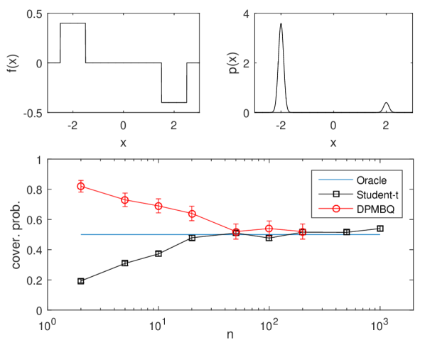
(a)

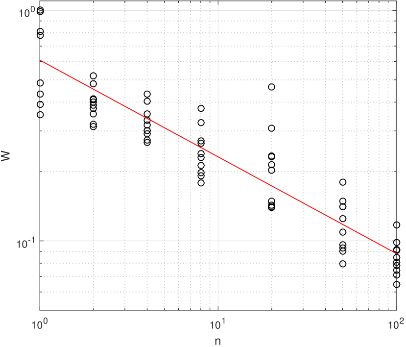
(b)

Figure 1: Simulated data results. (a) Comparison of coverage frequencies for the simulation experiments. (b) Convergence assessment: Wasserstein distance ($W$) between the posterior in Eqn. 11 and the true value of the integral, is presented as a function of the number $n$ of data points. [Circles represent independent realisations and the linear trend is shown in red.]

Empirical Results

Coverage frequencies are shown in Fig. 1(a) for a specific integration task $(f_{0},p_{0})$, that was deliberately selected to be difficult for Eqn. 12 due to the rare event represented by the mass at $x=2$. These were compared against central 50% posterior credible intervals produced under DPMBQ. These are the frequency with which the confidence/credible interval contain the true value of the integral, here estimated with 100 independent realisations for DPMBQ and 1000 for the (less computational) standard method (standard errors are shown for both). Whilst it offers correct coverage in the asymptotic limit, Eqn. 12 can be seen to be over-confident when $n$ is small, with coverage often less than $50\%$. In contrast, DPMBQ accounts for the fact $p$ is being estimated and provides conservative estimation about the extent of numerical error when $n$ is small.

To present results that do not depend on a fixed coverage level (e.g. 50%), we next measured convergence in the Wasserstein distance:

$$W=\int|p(f)-p_{0}(f_{0})|\;\mathrm{d}[p(f)\;|\;X,f(X)]$$

In particular we explored whether the theoretical rate of $n^{-1/4+\epsilon}$ was realised. (Note that the theoretical result applied just to fixed hyper-parameters, whereas the experimental results reported involved hyper-parameters that were marginalised, so that this is a non-trivial experiment.) Results in Fig. 1(b) demonstrated that $W$ scaled with $n$ at a rate which was consistent with the theoretical rate claimed.

Full experimental results on our polynomial test bed, reported in detail in the Supplemental Information, revealed that $W$ was larger for higher-degree polynomials (i.e. more complex integrands $f$), while $W$ was insensitive to the number of mixture components (i.e. to more complex distributions $p$). The latter observation may be explained by the fact that the kernel mean $\mu$ is a smoothed version of the distribution $p$ and so is not expected to be acutely sensitive to variation in $p$ itself.

3.2 Application to a Computational Cardiac Model

The Model

The computation model considered in this paper is due to Lee2016 and describes the mechanics of the left and right ventricles through a heart beat. In brief, the model geometry (Fig. 2(a), top right) is described by fitting a C¹ continuous cubic Hermite finite element mesh to segmented magnetic resonance images (MRI; Fig. 2(a), top left). Cardiac electrophysiology is modelled separately by the solution of the mono-domain equations and provides a field of activation times across the heart. The passive material properties and afterload of the heart are described, respectively, by a transversely isotropic material law and a three element Windkessel model. Active contraction is simulated using a phenomenological cellular model, with spatial variation arising from the local electrical activation times. The active contraction model is defined by five input parameters: $t_{r}$ and $t_{d}$ are the respective constants for the rise and decay times, $T_{0}$ is the reference tension, $a_{4}$ and $a_{6}$ respectively govern the length dependence of tension rise time and peak tension. These five parameters were concatenated into a vector $x\in\mathbb{R}^{5}$ and constitute the model inputs.

The model is fitted based on training data $y$ that consist of functionals $g_{j}:\mathbb{R}^{5}\rightarrow\mathbb{R}$, $j=1,\dots,10$, of the pressure and volume transient morphology during baseline activation and when the heart is paced from two leads implanted in the right ventricle apex and the left ventricle lateral wall. These 10 functionals are defined in the Supplemental Information; a schematic of the model and fitted measurements are shown in Fig. 2(a) (bottom panel).

Test Functions

The distribution $p(\mathrm{d}x)$ was taken to be the posterior distribution over model inputs $x$ that results from an improper flat prior on $x$ and a squared-error likelihood function: $\log p(x)=\text{const.}+\frac{1}{0.1^{2}}\sum_{j=1}^{10}(y_{j}-g_{j}(x))^{2}.$ The training data $y=(y_{1},\dots,y_{10})$ were obtained from clinical experiment. The task we considered is to compute posterior expectations for functionals $f(x)$ of the model output produced when the model input $x$ is distributed according to $p(\mathrm{d}x)$. This represents the situation where a fitted model is used to predict response to a causal intervention, representing a clinical treatment.

For assessment of the DPMBQ method, which is our principle aim in this experiment, we simply took the test functions $f$ to be each of the physically relevant model outputs $g_{j}$ in turn (corresponding to no causal intervention). This defined 10 separate numerical integration problems as a test bed. Benchmark values for $p_{0}(g_{j})$ were obtained, as described in the Supplemental Information, at a total cost of $\approx$ $10^{5}$ CPU hours, which would not be routinely practical.

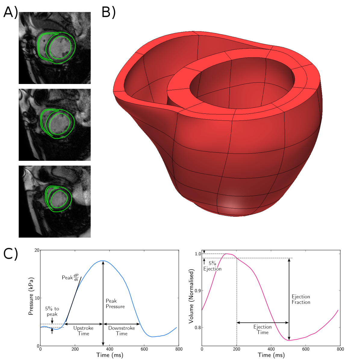
(a)

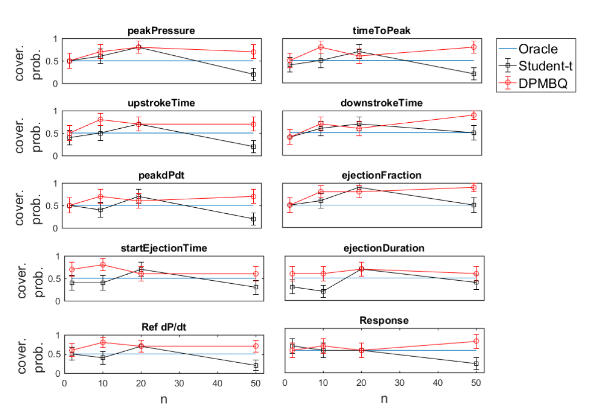
(b)

Figure 2: Cardiac model results: (a) Computational cardiac model. A) Segmentation of the cardiac MRI. B) Computational model of the left and right ventricles. C) Schematic image showing the features of pressure (left) and volume transient (right). (b) Comparison of coverage frequencies, for each of 10 numerical integration tasks defined by functionals $g_{j}$ of the cardiac model output.

Empirical Results

For each of the 10 numerical integration problems in the test bed, we computed coverage probabilities, estimated with 100 independent realisations (standard errors are shown), in line with those discussed for simulation experiments. These are shown in Fig. 2(b), where we compared Eqn. 12 with central 50% posterior credible intervals produced under DPMBQ. It is seen that Eqn. 12 is usually reliable but can sometimes be over-confident, with coverage probabilities less than $50\%$. This over-confidence can lead to spurious conclusions on the predictive performance of the computational model. In contrast, DPMBQ provides a uniformly conservative quantification of numerical error (cover. prob. $\geq 50\%$).

The DPMBQ method is further distinguished from Eqn. 12 in that it entails a joint distribution for the 10 integrals (the unknown $p$ is shared across integrals - an instance of transfer learning across the 10 integration tasks). Fig. 2(b) also appears to show a correlation structure in the standard approach (black lines), but this is an artefact of the common sample set $\{x_{i}\}_{i=1}^{n}$ that was used to simultaneously estimate all 10 integrals; Eqn. 12 is still applied independently to each integral.

4 Discussion

Numerical analysis often focuses the convergence order of numerical methods, but in non-asymptotic regimes the language of probabilities can provide a richer, more intuitive and more useful description of numerical error. This paper cast the computation of integrals $p(f)$ as an estimation problem amenable to Bayesian methods Kadane1985 ; Diaconis1988 ; Cockayne2017 . The difficulty of this problem depends on our level of prior knowledge (rendering the problem trivial if a closed-form solution is a priori known) and, in the general case, on how much information we are prepared to obtain on the objects $f$ and $p$ through numerical computation Hennig2015 . In particular, we distinguish between three states of prior knowledge: (1) $f$ known, $p$ unknown, (2) $f$ unknown, $p$ known, (3) both $f$ and $p$ unknown. Case (1) is the subject of Monte Carlo methods Robert2013 and concerns classical problems in applied probability such as estimating confidence intervals for expectations based on Markov chains. Notable recent work in this direction is Delyon2016 , who obtained a point estimate $\hat{p}$ for $p$ using a kernel smoother and then, in effect, used $\hat{p}(f)$ as an estimate for the integral. The decision-theoretic risk associated with error in $\hat{p}$ was explored in Cohen2016 . Independent of integral estimation, there is a large literature on density estimation Wand1994 . Our probabilistic approach provides a Bayesian solution to this problem, as a special case of our more general framework. Case (2) concerns functional analysis, where Novak2010 provide an extensive overview of theoretical results on approximation of unknown functions in an information complexity framework. As a rule of thumb, estimation improves when additional smoothness can be a priori assumed on the value of the unknown object (see Briol2016, ). The main focus of this paper was Case (3), until now unstudied, and a transparent, general statistical method called DPMBQ was proposed.

The path-finding nature of this work raises several important questions for future theoretical and applied research. First, these methods should be extended to account for the low-rank phenomenon that is often encountered in multi-dimensional integrals Dick2013 . Second, there is no reason, in general, to restrict attention to function values obtained at the locations in $X$. Indeed, one could first estimate $p(\mathrm{d}x)$, then select suitable locations $X^{\prime}$ from at which to evaluate $f(X^{\prime})$. This touches on aspects of statistical experimental design; the practitioner seeks a set $X^{\prime}$ that minimises an appropriate loss functional at the level of $p(f)$; see again Cohen2016 . Third, whilst restricted to Gaussians in our experiments, further methodological work will be required to establish guidance for the choice of kernel $k$ in the GP and choice of base distribution $P_{b}$ in the DPM (c.f. chapter 4 of Rasmussen2006, ).

There is an urgent ethical imperative to account for confounding due to numerical error in cardiac model assessment TJP:TJP7214 . To address this problem, we have proposed the DPMBQ method. However, the method should be of independent interest in machine learning for computer models in general (e.g. Gramacy2009, ).

Acknowledgments

CJO and MG were supported by the Lloyds Register Foundation Programme on Data-Centric Engineering. SN was supported by an EPSRC Intermediate Career Fellowship. FXB was supported by the EPSRC grant [EP/L016710/1]. MG was supported by the EPSRC grants [EP/K034154/1, EP/R018413/1, EP/P020720/1, EP/L014165/1], and an EPSRC Established Career Fellowship, [EP/J016934/1]. This material was based upon work partially supported by the National Science Foundation (NSF) under Grant DMS-1127914 to the Statistical and Applied Mathematical Sciences Institute. Opinions, findings, and conclusions or recommendations expressed in this material are those of the author(s) and do not necessarily reflect the views of the NSF.

Appendix A Supplemental Text

This supplement contains proofs, additional derivations and experimental results that complement the material in the Main Text.

A.1 Proof of Theorem

Denote by $p_{0}$ the true distribution that gives rise to the observations in $X$. Consider inference for $p_{0}$ under the DPM model for $X$. Let $\mu_{0}(x)=p_{0}(k(\cdot,x))\in\mathcal{H}$ denote the exact kernel mean. Let $\|\cdot\|_{\mathcal{H}}$ and $\langle\cdot,\cdot\rangle_{\mathcal{H}}$ denote the norm and inner product associated with $\mathcal{H}$. An important bound is derived from Cauchy-Schwarz:

$$\left|p_{0}(f_{0})-\sum_{i=1}^{n}w_{i}f_{0}(x_{i})\right|\leq\|f_{0}\|_{\mathcal{H}}\left\|\mu_{0}-\sum_{i=1}^{n}w_{i}k(\cdot,x_{i})\right\|_{\mathcal{H}}$$

This motivates us to study approximation of the kernel mean $\mu_{0}$ in a Hilbert space context. Let $\mu(x)=p(k(\cdot,x))\in\mathcal{H}$ be the generic unknown kernel mean in the case where $p$ is an uncertain distribution. The reproducing property in $\mathcal{H}$ can be used to bound kernel mean approximation error:

$$\|\mu_{0}-\mu\|_{\mathcal{H}}^{2} = \langle\mu_{0}-\mu,\mu_{0}-\mu\rangle_{\mathcal{H}}$$

$$= \left\langle\int k(\cdot,x)(p_{0}(x)-p(x))\mathrm{d}x,\right.$$

$$\left.\hskip 50.0pt\int k(\cdot,x^{\prime})(p_{0}(x^{\prime})-p(x^{\prime}))\mathrm{d}x^{\prime}\right\rangle_{\mathcal{H}}$$

$$= \iint\langle k(\cdot,x),k(\cdot,x^{\prime})\rangle_{\mathcal{H}}(p_{0}(x)-p(x))(p_{0}(x^{\prime})-p(x^{\prime}))\quad\mathrm{d}x\mathrm{d}x^{\prime}$$

$$\leq \sup_{x,x^{\prime}\in\Omega}|k(x,x^{\prime})|\times\|p_{0}-p\|_{1}^{2}$$

$$\leq 4\sup_{x,x^{\prime}\in\Omega}|k(x,x^{\prime})|\times d_{\text{Hell}}(p_{0},p)^{2}.$$

The DPM model provides a posterior distribution over $p(\mathrm{d}x)$; in turn this implies a posterior distribution over the kernel mean $\mu(x)$. Denote the Hellinger distance $d_{\text{Hell}}(p_{0},p)$ and recall that, for two densities $p_{0}$, $p$, we have $\|p_{0}-p\|_{1}\leq 2d_{\text{Hell}}(p_{0},p)$. Under assumptions (A2-5) of the theorem, (Ghosal2001, , Thm. 6.2) established that the DP location-scale mixture model satisfies $d_{\text{Hell}}(p_{0},p)=O_{P}(n^{-1/2+\epsilon})$, where $\epsilon>0$ denotes a generic positive constant that can be arbitrarily small. Thus, in the posterior, $\|\mu_{0}-\mu\|_{\mathcal{H}}^{2}=O_{P}(n^{-1+\epsilon})$.

Let $\mu_{0,n}(\cdot)=\mu_{0}(X)k(X,X)^{-1}k(X,\cdot)\in\mathcal{H}$. The idealised BQ posterior, where $p(\mathrm{d}x)$ is known, takes the form

$$[p(f)\;|\;p_{0},X,f_{0}(X)]=\text{N}(\langle f_{0},\mu_{0,n}\rangle_{\mathcal{H}},\|\mu_{0}-\mu_{0,n}\|_{\mathcal{H}}^{2}),$$

as shown in Briol2016 . Let $\mu_{n}(\cdot)=\mu(X)k(X,X)^{-1}k(X,\cdot)\in\mathcal{H}$. For the DPMBQ posterior, where $p(\mathrm{d}x)$ is unknown, we have the conditional distribution

$$[p(f)\;|\;p,X,f_{0}(X)]=\text{N}(\langle f_{0},\mu_{n}\rangle_{\mathcal{H}},\|\mu-\mu_{n}\|_{\mathcal{H}}^{2}).$$

Our aim is to relate the DPMBQ posterior to the idealised BQ posterior. To this end, it is claimed that:

$$\|\mu_{0}-\mu_{n}\|_{\mathcal{H}}^{2}\leq\|\mu_{0}-\mu_{0,n}\|_{\mathcal{H}}^{2}+n^{1/2}\|\mu_{0}-\mu\|_{\mathcal{H}}^{2}.$$ (13)

Here we have decomposed the estimation error $\mu_{0}-\mu_{n}$ into a term $\mu_{0}-\mu_{0,n}$, that represents the error of the idealised BQ method, and a term $\mu_{0}-\mu$ that captures the fact that the true mean element $\mu_{0}$ is unknown.

To prove the claim, we follow Lemma 2 in Briol2016 : Write $\epsilon(X)=\mu(X)-\mu_{0}(X)$ and deduce that

$$\|\mu_{0}-\mu_{n}\|_{\mathcal{H}}^{2}$$ (14)

$$= \left\|\int k(x,\cdot)p_{0}(\mathrm{d}x)-\mu(X)^{\top}k(X,X)^{-1}k(X,\cdot)\right\|_{\mathcal{H}}^{2}$$

$$= p_{0}\otimes p_{0}(k)-2\mu(X)^{\top}k(X,X)^{-1}\mu_{0}(X)+\mu(X)^{\top}k(X,X)^{-1}\mu(X)$$

$$= p_{0}\otimes p_{0}(k)-2(\epsilon(X)+\mu_{0}(X))^{\top}k(X,X)^{-1}\mu_{0}(X)$$

$$\hskip 50.0pt+(\epsilon(X)+\mu_{0}(X))^{\top}k(X,X)^{-1}(\epsilon(X)+\mu_{0}(X))$$

$$= p_{0}\otimes p_{0}(k)-2\mu_{0}(X)^{\top}k(X,X)^{-1}\mu_{0}(X)+\mu_{0}(X)^{\top}k(X,X)^{-1}\mu_{0}(X)$$

$$\hskip 50.0pt+\epsilon(X)^{\top}k(X,X)^{-1}\epsilon(X)$$

$$= \|\mu_{0}-\mu_{0,n}\|_{\mathcal{H}}^{2}+\epsilon(X)^{\top}k(X,X)^{-1}\epsilon(X).$$

Let $\mathcal{H}\otimes\mathcal{H}$ denote the tensor product of Hilbert spaces (Berlinet2011, , Sec. 1.4.6). Then the second term in Eqn. 14 is non-negative and can be bounded using the reproducing properties of both $\mathcal{H}$ and $\mathcal{H}\otimes\mathcal{H}$:

$$\epsilon(X)^{\top}k(X,X)^{-1}\epsilon(X) = \sum_{i,i^{\prime}=1}^{n}[k(X,X)^{-1}]_{i,i^{\prime}}\langle\mu-\mu_{0},k(\cdot,x_{i})\rangle_{\mathcal{H}}\langle\mu-\mu_{0},k(\cdot,x_{i^{\prime}})\rangle_{\mathcal{H}}$$

$$= \left\langle(\mu-\mu_{0})\otimes(\mu-\mu_{0}),\sum_{i,i^{\prime}=1}^{n}\begin{array}[]{ll}[k(X,X)^{-1}]_{i,i^{\prime}}\\ \hskip 30.0pt\times k(\cdot,x_{i})\otimes k(\cdot,x_{i^{\prime}})\end{array}\right\rangle_{\mathcal{H}\otimes\mathcal{H}}$$

$$\leq \|\mu_{0}-\mu\|_{\mathcal{H}}^{2}\left\|\sum_{i,i^{\prime}=1}^{n}[k(X,X)^{-1}]_{i,i^{\prime}}k(\cdot,x_{i})\otimes k(\cdot,x_{i^{\prime}})\right\|_{\mathcal{H}\otimes\mathcal{H}},$$

where the final inequality is Cauchy-Schwarz. The latter factor evaluates to $n^{1/2}$, again using the reproducing property for $\mathcal{H}\otimes\mathcal{H}$:

$$\left\|\sum_{i=1}^{n}\sum_{i^{\prime}=1}^{n}[k(X,X)^{-1}]_{i,i^{\prime}}k(\cdot,x_{i})\otimes k(\cdot,x_{i^{\prime}})\right\|_{\mathcal{H}\otimes\mathcal{H}}^{2}$$

$$= \sum_{i,i^{\prime},j,j^{\prime}}\begin{array}[]{ll}[k(X,X)^{-1}]_{i,i^{\prime}}[k(X,X)^{-1}]_{j,j^{\prime}}\\ \hskip 30.0pt\times\langle k(\cdot,x_{i})\otimes k(\cdot,x_{i^{\prime}}),k(\cdot,x_{j})\otimes k(\cdot,x_{j^{\prime}})\rangle_{\mathcal{H}\otimes\mathcal{H}}\end{array}$$

$$= \sum_{i,i^{\prime},j,j^{\prime}}[k(X,X)^{-1}]_{i,i^{\prime}}[k(X,X)^{-1}]_{j,j^{\prime}}[k(X,X)]_{i,j}[k(X,X)]_{i^{\prime},j^{\prime}}$$

$$= \text{tr}[k(X,X)k(X,X)^{-1}k(X,X)k(X,X)^{-1}]$$

$$= n.$$

This establishes that the claim holds.

From Lemmas 1 and 3 in Briol2016 , we have that the idealised BQ estimate based on the bounded kernel $k$ satisfies $\|\mu_{0}-\mu_{0,n}\|_{\mathcal{H}}=O_{P}(n^{-1/2})$. Indeed, $\|\mu_{0}-\mu_{0,n}\|_{\mathcal{H}}\leq\|\mu_{0}-\hat{\mu}_{0,n}\|_{\mathcal{H}}$, where

$$\hat{\mu}_{0,n}=\frac{1}{n}\sum_{i=1}^{n}k(\cdot,x_{i})$$

is the Monte Carlo estimate for the kernel mean (Lemma 3 of Briol2016, ). As $k$ is bounded, the norm $\|\mu_{0}-\hat{\mu}_{0,n}\|_{\mathcal{H}}$ vanishes as $O_{P}(n^{-1/2})$ (Lemma 1 of Briol2016, ). Combining the above results in Eqn. 13, we obtain

$$\|\mu_{0}-\mu_{n}\|_{\mathcal{H}}^{2} = O_{P}(n^{-1})+n^{1/2}\times O_{P}(n^{-1+\epsilon})$$

$$= O_{P}(n^{-1/2+\epsilon}).$$

To finish, recall that for DPMBQ we have the random variable representation

$$p(f) = \langle f_{0},\mu_{n}\rangle_{\mathcal{H}}+\|\mu-\mu_{n}\|_{\mathcal{H}}\;\xi,$$

where $\xi\sim\text{N}(0,1)$ is independent of $X$. Thus, from the triangle inequality followed by Cauchy-Schwarz:

$$|p_{0}(f_{0})-p(f)| = |\langle f_{0},\mu_{0}\rangle_{\mathcal{H}}-\langle f_{0},\mu_{n}\rangle_{\mathcal{H}}-\|\mu-\mu_{n}\|_{\mathcal{H}}\;\xi|$$

$$\leq |\langle f_{0},\mu_{0}-\mu_{n}\rangle_{\mathcal{H}}|+\|\mu-\mu_{n}\|_{\mathcal{H}}\;|\xi|$$

$$\leq |\langle f_{0},\mu_{0}-\mu_{n}\rangle_{\mathcal{H}}|+[\|\mu-\mu_{0}\|_{\mathcal{H}}+\|\mu_{0}-\mu_{n}\|_{\mathcal{H}}]\;|\xi|$$

$$\leq \|f_{0}\|_{\mathcal{H}}\|\mu_{0}-\mu_{n}\|_{\mathcal{H}}+O_{P}(n^{-1/2+\epsilon})+O_{P}(n^{-1/4+\epsilon})$$

$$= O_{P}(n^{-1/4+\epsilon}).$$

Denote the DPMBQ posterior distribution with $\mathbb{P}_{n}=[p(f)\;|\;X,f(X)]$. Then for $\delta>0$ fixed, the posterior mass $\mathbb{P}_{n}[(\infty,p_{0}(f_{0})-\delta)\cup(p_{0}(f_{0})+\delta,\infty)]=O_{P}(n^{-1/4+\epsilon})$. This completes the proof.

A.2 Computational Details

This section describes the computation for DPMBQ. The model admits the following straight-forward sampler:

1. draw $\theta$ from the hyper-prior $[\theta]$

2. draw $\phi_{1:n}$ from $[\phi_{1:n}\;|\;X,\theta]$ (via a Gibbs sampler)

3. draw $p$ from $[\mathrm{d}p\;|\;\phi_{1:n}]$ (via stick-breaking)

4. draw $p(f)$ from $[p(f)\;|\;X,f(X),p,\theta]$ (via BQ)

For step (2), it is convenient (but not essential) to use a conjugate base distribution $P_{b}$. In the case of a Gaussian model $\psi$, the normal inverse-gamma distribution, parametrised with $\mu_{0}\in\mathbb{R}$, $\lambda_{0},\alpha_{0},\beta_{0}\in(0,\infty)$, permits closed-form conditionals and facilitates an efficient Gibbs sampler. Full details are provided in supplemental Sec. A.2.1. (Note that the conjugate base distribution does not fall within the scope of the theorem; however the use of a more general Metropolis-within-Gibbs scheme enables computation from such models with trivial modification.) In all experiments below we fixed hyper-parameters to default values $\lambda_{0}=\alpha_{0}=\beta_{0}=1$, $\mu_{0}=0$; there was no noticeable dependence of inferences on these choices, which are several levels removed from $p(f)$, the unknown of interest.

This direct scheme admits several improvements: e.g. (a) stratified or QMC sampling of $\theta$ in step (1); (b) Rao-Blackwellisation of the additional randomisation in $p(f)$, to collapse steps (3) and (4) Blackwell1947 ; (c) the Gibbs sampler of Escobar1995 can be replaced by more sophisticated alternatives, such as Neal2000 . Indeed, one need not sample from the prior $[\theta]$ and instead target the hyper-parameter posterior with MCMC. In experiments, the straight-forward scheme outlined here was more than adequate to obtain samples from the DPMBQ model. Thus we implemented this basic sampler and leave the above extensions as possible future work.

A.2.1 Gibbs Sampler

This section derives the conditional distributions that are needed for an efficient Gibbs sampler that targets $[\phi\;|\;X,\theta]$. The main result is presented in the proposition below:

Proposition.

Consider the multivariate Gaussian model $\psi(\mathrm{d}x;\phi)=\text{\emph{N}}(\mathrm{d}x|\phi_{1},\text{\emph{diag}}(\phi_{2}))$, with mean vector $\phi_{1}\in\mathbb{R}^{d}$ and marginal variance vector $\phi_{2}\in\mathbb{R}^{d}$. Consider the base distribution $P_{b}(\mathrm{d}\phi)$ composed of independent normal inverse-gamma $\text{\emph{NIG}}(\phi_{1,k},\phi_{2,k}|\mu_{0},\lambda_{0},\alpha_{0},\beta_{0})$ components with $\mu_{0}\in\mathbb{R}$, $\lambda_{0},\alpha_{0},\beta_{0}\in(0,\infty)$ for $k=1,\dots,d$. Denote $\phi_{i}=(\phi_{i,1},\phi_{i,2})$ and $\phi_{(-i)}=(\phi_{1},\dots,\phi_{i-1},\phi_{i+1},\dots,\phi_{n})$. For this conjugate choice, we have the closed-form posterior conditional

$$[\phi_{i}\;|\;\phi_{(-i)},X,\theta]=\omega_{0}Q_{i}+\sum_{j\neq i}\omega_{j}\delta_{\phi_{j}}$$

where $Q_{i}$ is composed of independent $\text{\emph{NIG}}(\phi_{i,1,k},\phi_{i,2,k}|\mu_{i,k},\lambda_{i,k},\alpha_{i,k},\beta_{i,k})$ components and

$$\left[\begin{array}[]{c}\omega_{0}\\ \omega_{j}\end{array}\right] \propto \left[\begin{array}[]{c}\alpha\prod_{k=1}^{d}\frac{1}{2\pi^{1/2}}\frac{\lambda_{0}^{1/2}}{\lambda_{i,k}^{1/2}}\frac{\beta_{0}^{\alpha_{0}}}{\beta_{i,k}^{\alpha_{i,k}}}\frac{\Gamma(\alpha_{i,k})}{\Gamma(\alpha_{0})}\\ \text{\emph{N}}(x_{i}|\phi_{j,1},\text{\emph{diag}}(\phi_{j,2}))\end{array}\right]$$

$$\mu_{i,k} = \frac{\lambda_{0}\mu_{0}+x_{i,k}}{\lambda_{0}+1}$$

$$\lambda_{i,k} = \lambda_{0}+1$$

$$\alpha_{i,k} = \alpha_{0}+\frac{1}{2}$$

$$\beta_{i,k} = \beta_{0}+\frac{1}{2}(\lambda_{0}\mu_{0}^{2}+x_{i,k}^{2}-\lambda_{i,k}\mu_{i,k}^{2}).$$

Proof.

From Theorem 1 of Ferguson1973 , also known as “Bayes’ theorem for DPs”, we have that the prior $P\sim\text{DP}(\alpha,P_{b})$ and the likelihood $\phi_{i}\sim P$ (independent) lead to a posterior

$$P\;|\;\phi_{(-i)}\sim\text{DP}\left(\alpha+n-1,\frac{1}{\alpha+n-1}\left(\alpha P_{b}+\sum_{j\neq i}\delta_{\phi_{j}}\right)\right).$$

It follows that, for a measurable set $A$,

$$\text{Prob}[\phi_{i}\in A\;|\;\phi_{(-i)}] = \mathbb{E}[P(A)\;|\;\phi_{(-i)}]$$

$$= \frac{1}{\alpha+n-1}\left(\alpha P_{b}(A)+\sum_{j\neq i}\delta_{\phi_{j}}(A)\right).$$

From (standard) Bayes’ theorem,

$$[\phi_{i}\;|\;\phi_{(-i)}] = \frac{[X\;|\;\phi_{1:n}]\;[\phi_{i}\;|\;\phi_{(-i)}]}{[X\;|\;\phi_{(-i)}]}$$

$$\propto [X\;|\;\phi_{1:n}]\;[\phi_{i}\;|\;\phi_{(-i)}]\;\propto\;[x_{i}\;|\;\phi_{i}]\;[\phi_{i}\;|\;\phi_{(-i)}]$$

and combining the two above results, in the case of a Gaussian model $\psi(\mathrm{d}x_{i};\phi_{i})$ with mean vector $\phi_{i,1}$ and marginal variance vector $\phi_{i,2}$, leads to

$$[\phi_{i}\;|\;\phi_{(-i)}] \propto \text{N}(x_{i}|\phi_{i,1},\text{diag}(\phi_{i,2}))\times\left(\alpha P_{b}(\phi_{i})+\sum_{j\neq i}\delta_{\phi_{j}}(\phi_{i})\right)$$

$$= \alpha\text{N}(x_{i}|\phi_{i,1},\text{diag}(\phi_{i,2}))P_{b}(\phi_{i})+\sum_{j\neq i}\text{N}(x_{i}|\phi_{j,1},\text{diag}(\phi_{j,2}))\delta_{\phi_{j}}(\phi_{i}),$$

where $\phi_{i}=(\phi_{i,1},\phi_{i,2})$ with $\phi_{i,1}\in\mathbb{R}^{d}$ and $\phi_{i,2}\in(0,\infty)^{d}$.

For closed-form expressions, $P_{b}$ must be taken conjugate to the Gaussian model:

$$P_{b}(\phi_{i}) = \prod_{k=1}^{d}\text{NIG}(\phi_{i,1,k},\phi_{i,2,k}|\mu_{0},\lambda_{0},\alpha_{0},\beta_{0})$$

$$= \prod_{k=1}^{d}\text{N}(\phi_{i,1,k}|\mu_{0},\lambda_{0}^{-1}\phi_{i,2,k})\text{IG}(\phi_{i,2,k}|\alpha_{0},\beta_{0}),$$

in the obvious notation $\phi_{i,j}=(\phi_{i,j,1},\dots,\phi_{i,j,d})$. Thus

$$\text{N}(x_{i}|\phi_{i,1},\text{diag}(\phi_{i,2}))P_{b}(\phi_{i}) = \text{N}(x_{i}|\phi_{i,1},\text{diag}(\phi_{i,2}))$$

$$\hskip 50.0pt\times\prod_{k=1}^{d}\text{NIG}(\phi_{i,1,k},\phi_{i,2,k}|\mu_{0},\lambda_{0},\alpha_{0},\beta_{0})$$

$$= \omega_{0}\times\prod_{k=1}^{d}\text{NIG}(\phi_{i,1,k},\phi_{i,2,k}|\mu_{i,k},\lambda_{i,k},\alpha_{i,k},\beta_{i,k}),$$

where

$$\omega_{0} = \prod_{k=1}^{d}\frac{1}{2\pi^{1/2}}\frac{\lambda_{0}^{1/2}}{\lambda_{i,k}^{1/2}}\frac{\beta_{0}^{\alpha_{0}}}{\beta_{i,k}^{\alpha_{i,k}}}\frac{\Gamma(\alpha_{i,j})}{\Gamma(\alpha_{0})}$$

$$\mu_{i,k} = \frac{\lambda_{0}\mu_{0}+x_{i,k}}{\lambda_{0}+1}$$

$$\lambda_{i,k} = \lambda_{0}+1$$

$$\alpha_{i,k} = \alpha_{0}+\frac{1}{2}$$

$$\beta_{i,k} = \beta_{0}+\frac{1}{2}(\lambda_{0}\mu_{0}^{2}+x_{i,k}^{2}-\lambda_{i,k}\mu_{i,k}^{2}).$$

This completes the proof. ∎

In all experiments the Gibbs sampler was initialised at $\phi_{i,1,k}=x_{i,k}$ and $\phi_{i,2,k}=1$ and run until a convergence criteria was satisfied. In this way we produced samples from $[\phi_{1:n}\;|\;X,\theta]$ for the direct sampling scheme outlined in the main text.

A.2.2 Tensor Structure for Multi-Dimensional Integrals

This section describes how multi-dimensional integration problems on a tensor-structured domain $\Omega=\Omega_{1}\otimes\dots\otimes\Omega_{d}$ can be decomposed into a tensor product of univariate integration problems. This construction was used to produce the results in the Main Text, as well as in Sec. A.3.2 of the Supplement.

Assume a tensor product kernel

$$k(x,x^{\prime})=k_{1}(x_{1},x_{1}^{\prime})\times\dots\times k_{d}(x_{d},x_{d}^{\prime})$$

on $\Omega\times\Omega$, together with a product model

$$\psi(\mathrm{d}x;\phi)=\psi_{1}(\mathrm{d}x_{1};\phi_{1})\times\dots\times\psi_{d}(\mathrm{d}x_{d};\phi_{d}).$$

Then a generic draw from $[p\;|\;\phi_{1:n}]$ has the form

$$p(\mathrm{d}x)=\sum_{j=1}^{\infty}w_{j}\psi_{1}(\mathrm{d}x_{1};\varphi_{j,1})\times\dots\times\psi_{d}(\mathrm{d}x_{d};\varphi_{j,d}),$$

where $\varphi_{j}\sim P$ are independent with $\varphi_{j}=(\varphi_{j,1},\dots,\varphi_{j,d})$, and the corresponding kernel mean is

$$\mu(x)=\sum_{j=1}^{\infty}w_{j}\prod_{i=1}^{d}\left(\int_{\Omega_{i}}k_{i}(x_{i},x_{i}^{\prime})\psi_{i}(x_{i}^{\prime};\varphi_{j,i})\mathrm{d}x_{i}^{\prime}\right).$$

The initial error $p\otimes p(k)$ is derived as

$$p\otimes p(k) = \sum_{j,j^{\prime}=1}^{\infty}w_{j}w_{j^{\prime}}\prod_{i=1}^{d}$$

$$\int_{\Omega_{i}}k_{i}(x_{i},x_{i}^{\prime})\psi_{i}(x_{i};\varphi_{j,i})\psi_{i}(x_{i}^{\prime};\varphi_{j,i})\mathrm{d}x_{i}\mathrm{d}x_{i}^{\prime}.$$

For an efficient Gibbs sampler, as in Sec. A.2.1, the prior model on the mixing distribution $P(\mathrm{d}\phi)$ was taken as a tensor product of $\text{DP}(\alpha,P_{b,i})$ priors where $P_{b,i}(\mathrm{d}x_{i})$ is a base distribution on $\Omega_{i}$. The experiments of Sec. A.3.2 were performed as explained above, where the individual components $k_{i}$, $\psi_{i}$ and $P_{b,i}$ were taken to be the same as used for the simulation examples in Sec. A.3.

A.3 Experimental Set-Up and Results

Two simulation studies were undertaken, based on polynomial test functions where the true integral is known in closed-form (Sec. A.3.1) and based on differential equations where the true integral must be estimated with brute-force computation (Sec. A.3.2).

A.3.1 Flexible Polynomial Test Bed

To assess the performance of the DPMBQ method, we considered independent data $x_{1},\dots,x_{n}$ generated from a known distribution $p(\mathrm{d}x)$. In addition, the function $f(x)$ was fixed and known, so that overall the exact value of the integral $p(f)$ provided a known benchmark.

For illustration, we focused on the generic class of one-dimensional test problems obtained when $p(\mathrm{d}x)$ is a Gaussian mixture distribution

$$p(\mathrm{d}x)=\sum_{i=1}^{m}r_{i}\mathrm{N}(\mathrm{d}x;c_{i},s_{i}^{2})$$

defined on $\Omega=\mathbb{R}$, where $c_{i}\in\mathbb{R}$, $r_{i},s_{i}\in[0,\infty)$, $\sum_{i=1}^{m}r_{i}=1$, and the function $f(x)$ is a polynomial

$$f(x)=\sum_{i=1}^{q}a_{i}x^{b_{i}}$$

where $a_{i}\in\mathbb{R}$ and $b_{i}\in\mathbb{N}_{0}$. For this problem class, the integral $p(f)$ is computable in closed-form and the generic approximation properties of Gaussian mixtures and polynomials provide an expressive test-bed. In addition, the GP prior with mean function $m_{\theta}(x)=0$ and Gaussian covariance function

$$k_{\theta}(x,x^{\prime})=\zeta\exp(-(x-x^{\prime})^{2}/2\lambda^{2})$$

was employed with $\zeta=1$ fixed. This choice provides a closed-form kernel mean for assessment purposes, with standard Gaussian calculations analogous to those performed in the Main Text.

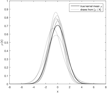
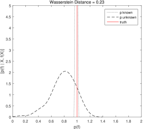
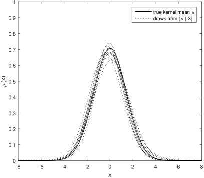
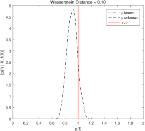
Figure 3: Illustration; computation of $p(f)$ where both $f(x)$ and $p(\mathrm{d}x)$ are a priori unknown. Partial information on $p(\mathrm{d}x)$ is provided as $n$ draws $x_{i}\sim p(\mathrm{d}x)$. Partial information on $f(x)$ is provided by the values $f(x_{i})$ at each of the $n$ locations. Left: Bayesian estimation of the kernel mean $\mu$, that characterises the unknown distribution $p(\mathrm{d}x)$. Right: Posterior distribution over the value of the integral $p(f)$ (dashed line); for reference, the truth (red line) and the posterior that would be obtained if $p(\mathrm{d}x)$ was known (dotted line) are also shown. Two sample sizes, (top) $n=10$, (bottom) $n=100$, are presented.

Illustration

Consider the toy problem where $f(x)=1+x-0.1x^{3}$, $p(\mathrm{d}x)=\text{N}(\mathrm{d}x;0,1)$, such that the true integral $p(f)=1$ is known in closed-form. For the kernel $k_{\theta}$ we initially fixed the hyper-parameter $\lambda$ at a default value $\lambda=1$. The concentration hyper-parameter $\alpha$ was initially fixed to $\alpha=1$ (the unit information DP prior). For all experiments, the stick breaking construction described in the Main Text was truncated after the first $N=500$ terms; at this level results were invariant to further increases in $N$. In Fig. 3 we present realisations of the posterior distributions $[\mu\;|\;X]$ and $[p(f)\;|\;X,f(X)]$ at two sample sizes, (a) $n=10$ and (b) $n=100$. In this case each posterior contains the true value $p_{0}(f_{0})$ of the integral in its effective support region. The posterior variance is greatly inflated with respect to the idealised case in which $p(\mathrm{d}x)$, and hence the kernel mean $\mu$, is known. This is intuitively correct and reflects the increased difficulty of the problem in which both $f(x)$ and $p(\mathrm{d}x)$ are a priori unknown.

Detailed Results

To explore estimator convergence in detail, we considered the general simulation set-up above and measured estimator performance with the Wasserstein (or earth movers’) distance:

$$W=\int|p(f)-p_{0}(f_{0})|\;\mathrm{d}[p(f)\;|\;X,f(X)].$$

Consistent estimation, as defined in the Main Text, is implied by convergence in Wasserstein distance. It should be noted that consistent estimation does not imply correct coverage of posterior credible intervals Ghosal2007 ; this aspect is left for future work.

There are three main questions that we address below; these concern dependence of the approximation properties of the posterior $[p(f)\;|\;X,f(X)]$ on (i) the number $n$ of data, (ii) the complexity of the distribution $p(\mathrm{d}x)$, and (iii) the complexity of the function $f(x)$. Our results can be summarised as follows:

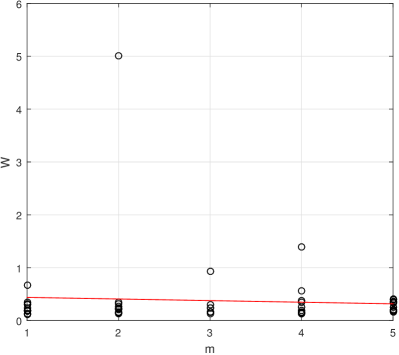
Figure 4: Empirical investigation. The Wasserstein distance, $W$, between the posterior $[p(f)\;|\;X,f(X)]$ and the true value of the integral is presented as a function of (left) the number $m$ of mixture components that constitute $p(\mathrm{d}x)$, and (right) the degree $q$ of the polynomial function $f(x)$ whose integral is to be determined. [Circles represent independent realisations of $W$, while in (right) a linear trend line (red) is shown.]

• Effect of the number $n$ of data: As $n$ increases, we expect contraction of the posterior measure over $[\mu\;|\;X]$ onto the true kernel mean. Hence, in the limit of infinite data, the resultant integral estimates will coincide with those of BQ. However, the rate of convergence of the proposed method could be much slower compared to the idealised case in which $p(\mathrm{d}x)$, and hence $\mu(x)$, is a priori known.

  The problem of Fig. 3 was considered in a more general setting where the hyper-parameters $\theta$ are assigned prior distributions and are subsequently marginalised out. For these results, the kernel parameter $\lambda$ was assigned a $\text{Gam}(2,1)$ hyper-prior and the concentration parameter $\alpha$ was assigned a $\text{Exp}(1)$ hyper-prior; these were employed for the remainder.

  Results in Fig. 5 showed that the posterior $[p(f)\;|\;X,f(X)]$ appears to converge to the true value of the integrand (in the Wasserstein sense) as the number $n$ of data are increased. The slope of the trend line was $\approx-1/4$, in close agreement with the theoretical analysis. This does not resemble the rapid posterior contraction results established in BQ when $p(\mathrm{d}x)$ is a priori known, which can be exponential for the Gaussian kernel Briol2016 . This reflects the more challenging nature of the estimation problem when $p(\mathrm{d}x)$ is unavailable in closed-form.

• Effect of the complexity of $p(\mathrm{d}x)$: It is anticipated that a more challenging inference problem for $p(\mathrm{d}x)$ entails poorer estimation performance for $p(f)$. To investigate, the complexity of $p(\mathrm{d}x)$ was measured as the number $m$ of mixture components. For this experiment, the number $m$ of mixture components was fixed, with weights $(r_{1},\dots,r_{m})$ drawn from $\text{Dir}(2)$. The location parameters $c_{i}$ were independent draws from $\text{N}(0,1)$ and the scale parameters $s_{i}$ were independent draws from $\text{Exp}(1)$.

  Results in Fig. 4 (left), which were based on $n=20$, did not demonstrate a clear effect. This was interesting and can perhaps be explained by the fact that $\mu(x)$ is a kernel-smoothed version of $p(\mathrm{d}x)$ and thus is somewhat robust to fluctuations in $p(\mathrm{d}x)$.

• Effect of the complexity of $f(x)$: A more challenging inference problem for $f(x)$ ought to also entails poorer estimation. To investigate, the complexity of $f(x)$ was measured as the degree $q$ of this polynomial. For each experiment, $q$ was fixed and the coefficients $a_{i}$ were independent draws from $\text{N}(0,1)$.

  Results in Fig. 4 (right), based on $n=20$, showed that the posterior was more accurate for larger $q$, this time in agreement with intuition.

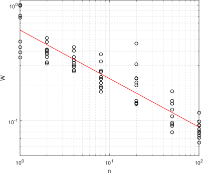
Figure 5: Empirical investigation. The example of Fig. 3 was again considered, this time marginalising over hyper-parameters $\lambda$ and $\alpha$. The Wasserstein distance, $W$, between the posterior $[p(f)\;|\;X,f(X)]$ and the true value of the integral, is presented as a function of the number $n$ of data points. [Circles represent independent realisations, while a linear trend line (red) is shown.]

A.3.2 Goodwin Oscillator

Our second simulation experiment considered the computation of Bayesian forecasts based on a 5-dimensional computer model.

For a manageable benchmark we took a computer model that is well-understood; the Goodwin oscillator, which is prototypical for larger models of complex chemical systems Goodwin1965 . The oscillator considers a competitive molecular dynamic, expressed as a system of ordinary differential equations (ODEs), that induces oscillation between the concentration $z_{i}(t;x)$ of two species $S_{i}$ ($i=1,2$). Parameters, denoted $x$ and a priori unknown, included two synthesis rate constants, two degradation rate constants and one exponent parameter. Full details, that include the prior distributions over parameters used in the experiment below, can be found in Oates2016 . From an experimental perspective, we suppose that concentrations of both species are observed at 41 discrete time points $t_{j}$ with uniform spacing in $[0,40]$. Observation occurred through an independent Gaussian noise process $y_{i,j}=z_{i}(t_{j};x)+\epsilon_{i,j}$ where $\epsilon_{i,j}\sim\text{N}(0,0.1^{2})$. Data-generating parameters were identical to Oates2016 with model dimension $g=3$. Fig. 6 (left) shows the full data $y=(y_{i,j})$.

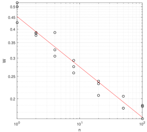
Figure 6: Application to Bayesian forecasting. Left: Data on two species, $S_{1}$ and $S_{2}$, generated from the Goodwin oscillator, a system of differential equations that contain five unknown parameters. The forecast $p(f)$ under consideration is the posterior expected concentration of species $S_{1}$ at the later time point $t=50$. Right: The Wasserstein distance, $W$, from the proposed posterior $[p(f)\;|\;X,f(X)]$ to the true integral is shown. Here $n$ represents the number of samples $x_{i}$ that were obtained from the posterior $[x\;|\;y]$ over the unknown parameters.

The forecast that we consider here is for the concentration of $S_{1}$ at the later time $t=50$. In particular we defined $f(x)$ to be equal to $z_{1}(50)$ and obtained $n$ samples $x_{i}$ from the posterior $[x\;|\;y]$ using tempered population Markov chain Monte Carlo (MCMC), in all aspects identical to Oates2016 . Then, $f(x_{i})$ was evaluated and stored for each $x_{i}$; the locations $X=(x_{i})$ and function evaluations $f(X)$ are the starting point for the DPMBQ method.

This prototypical model is small enough for numerical error to be driven to zero via repeated numerical simulation of the ODEs, providing us with a benchmark. Nevertheless, the key features that motivate our work are present here: (i) The forecast function $f(x)$ is expensive and black-box, being a long-range solution of a system of ODEs and requiring that the global solution error is carefully controlled. (ii) The task of obtaining samples $x_{i}$ is costly, as each evaluation of the likelihood $[y\;|\;x]$, and hence the posterior $[x\;|\;y]$, requires the solution of a system of ODEs.

Performance was examined through the Wasserstein distance to the true forecast $p_{0}(f_{0})$, the latter obtained through brute-force simulation. The multi-dimensional integral was modelled as a tensor product of one-dimensional integrals, as described in Sec. A.2.2 in the supplement. This allowed the uni-variate model from Sec. A.3 to be re-used at minimal effort. Results, in Fig. 6 (right), indicated that the posterior was consistent. Note that the Wasserstein distances are large for this problem, reflecting the greater uncertainties that are associated with a 5-dimensional integration problem with only $n<10^{2}$ draws from $p(\mathrm{d}x)$.

An extension of this framework, not considered here, would use a probabilistic ODE solver in tandem with DPMBQ to model the approximate nature of numerical solution to the ODEs in the reported forecasts Skilling1992 ; Hennig2015 .

A.3.3 Cardiac Model Experiment

Test Functionals $g_{j}$ Used in the Cardiac Model Experiment

The 10 functionals $g_{j}$, that are the basis for clinical data on the cardiac model in the main text, are defined in the next paragraph:

The left ventricle pressure curve during baseline activation is characterised by the peak value (Peak Pressure), the time of the peak value (Time to Peak) and the time for pressure to rise (Upstroke Time) from 5% of the pressure change to the peak value and then fall back down (Down Stroke Time). The volume transient is described by the ratio of the left ventricle volume of blood ejected over the maximal left ventricle volume (Ejection Fraction), the time that the ventricle volume has decreased by 5% of the maximal volume (Start Ejection Time) and the time taken between the start of ejection and the point where the heart reaches its smallest left ventricle volume (Ejection Duration). The effect of pacing the heart is measured by the percentage change in the maximum rate of pressure development at baseline (Ref dPdt) and during pacing (Peak dPdt), defined as the acute haemodynamic response (Response).

Brute-Force Computation for a Benchmark

The samples $\{x_{i}\}_{i=1}^{n}$ from $p(\mathrm{d}x)$ can in principle be obtained via any sophisticated Markov chain Monte Carlo (MCMC) methods, such as Strathmann2015 ; Conrad2016 . Recall that each evaluation of $p(\mathrm{d}x)$ requires $\approx 10^{3}$ hours, so that the MCMC method must be efficient. To reduce the computational overhead required for this project, we circumvented MCMC and instead exploited an existing, detailed empirical approximation to $p(\mathrm{d}x)$ that had been pre-computed by a subset of the authors. This consisted of a collection of $m\approx 10^{3}$ weighted states $(x_{i},p_{i})$, where the $x_{i}$ were selected via an ad-hoc adaptive Latin hypercube method, and such that the weights $p_{i}\propto p(x_{i})$. Then, in this work, an (approximate) sample of size $n\ll m$ was obtained by sampling with replacement from the empirical distribution defined by this weighted point set. For our assessment of DPMBQ, benchmark values for each integral were computed as $\Sigma_{i=1}^{m}p_{i}f(x_{i})$ for $m\approx 10^{3}$; note that this required a total of $\approx$ $10^{5}$ CPU hours and would not be routinely practical.

References

- [1] F Bach. On the Equivalence Between Quadrature Rules and Random Features. arXiv:1502.06800, 2015.
- [2] A Berlinet and C Thomas-Agnan. Reproducing Kernel Hilbert Spaces in Probability and Statistics. Springer Science & Business Media, 2011.
- [3] D Blackwell. Conditional Expectation and Unbiased Sequential Estimation. Annals of Mathematical Statistics, 18(1):105–110, 1947.
- [4] F-X Briol, CJ Oates, M Girolami, and MA Osborne. Frank-Wolfe Bayesian quadrature: Probabilistic integration with theoretical guarantees. In Advances in Neural Information Processing Systems, pages 1162–1170, 2015.
- [5] F-X Briol, CJ Oates, M Girolami, MA Osborne, and D Sejdinovic. Probabilistic Integration: A Role for Statisticians in Numerical Analysis? arXiv:1512.00933, 2015.
- [6] J Cockayne, CJ Oates, T Sullivan, and M Girolami. Bayesian probabilistic numerical methods. arXiv:1702.03673, 2017.
- [7] SN Cohen. Data-driven nonlinear expectations for statistical uncertainty in decisions. arXiv:1609.06545, 2016.
- [8] Patrick R Conrad, Youssef M Marzouk, Natesh S Pillai, and Aaron Smith. Accelerating asymptotically exact mcmc for computationally intensive models via local approximations. Journal of the American Statistical Association, 111(516):1591–1607, 2016.
- [9] PS Craig, M Goldstein, JC Rougier, and AH Seheult. Bayesian Forecasting for Complex Systems Using Computer Simulators. Journal of the American Statistical Association, 96(454):717–729, 2001.
- [10] B Delyon and F Portier. Integral Approximation by Kernel Smoothing. Bernoulli, 22(4):2177–2208, 2016.
- [11] P Diaconis. Bayesian Numerical Analysis. Statistical Decision Theory and Related Topics IV, 1:163–175, 1988.
- [12] P Diaconis and D Freedman. On the Consistency of Bayes Estimates. Annals of Statistics, 14(1):1–26, 1986.
- [13] J Dick, FY Kuo, and IH Sloan. High-Dimensional Integration: The Quasi-Monte Carlo Way. Acta Numerica, 22:133–288, 2013.
- [14] MD Escobar and M West. Bayesian Density Estimation and Inference Using Mixtures. Journal of the American Statistical Association, 90(430):577–588, 1995.
- [15] TS Ferguson. A Bayesian Analysis of Some Nonparametric Problems. Annals of Statistics, 1(2):209–230, 1973.
- [16] TS Ferguson. Bayesian Density Estimation by Mixtures of Normal Distributions. Recent Advances in Statistics, 24(1983):287–302, 1983.
- [17] Z Ghahramani and CE Rasmussen. Bayesian Monte Carlo. In Advances in Neural Information Processing Systems, volume 15, pages 489–496, 2002.
- [18] S Ghosal and A Van Der Vaart. Convergence Rates of Posterior Distributions for Non-IID Observations. Annals of Statistics, 35(1):192–223, 2007.
- [19] S Ghosal and AW Van Der Vaart. Entropies and Rates of Convergence for Maximum Likelihood and Bayes Estimation for Mixtures of Normal Densities. Annals of Statistics, 29(5):1233–1263, 2001.
- [20] BC Goodwin. Oscillatory Behavior in Enzymatic Control Processes. Advances in Enzyme Regulation, 3:425–437, 1965.
- [21] RB Gramacy and HKH Lee. Adaptive Design and Analysis of Supercomputer Experiments. Technometrics, 51(2):130–145, 2009.
- [22] T Gunter, MA Osborne, R Garnett, P Hennig, and SJ Roberts. Sampling for Inference in Probabilistic Models With Fast Bayesian Quadrature. In Advances in Neural Information Processing Systems, pages 2789–2797, 2014.
- [23] P Hennig, MA Osborne, and M Girolami. Probabilistic Numerics and Uncertainty in Computations. Proceedings of the Royal Society A, 471(2179):20150142, 2015.
- [24] F Huszár and D Duvenaud. Optimally-Weighted Herding is Bayesian Quadrature. In Uncertainty in Artificial Intelligence, volume 28, pages 377–386, 2012.
- [25] H Ishwaran and LF James. Gibbs Sampling Methods for Stick-Breaking Priors. Journal of the American Statistical Association, 96(453):161–173, 2001.
- [26] H Ishwaran and M Zarepour. Exact and Approximate Sum Representations for the Dirichlet Process. Canadian Journal of Statistics, 30(2):269–283, 2002.
- [27] JB Kadane and GW Wasilkowski. Average case epsilon-complexity in computer science: A Bayesian view. Bayesian Statistics 2, Proceedings of the Second Valencia International Meeting, pages 361–374, 1985.
- [28] M Kanagawa, BK Sriperumbudur, and K Fukumizu. Convergence Guarantees for Kernel-Based Quadrature Rules in Misspecified Settings. In Advances in Neural Information Processing Systems, volume 30, 2016.
- [29] T Karvonen and S Särkkä. Fully symmetric kernel quadrature. arXiv:1703.06359, 2017.
- [30] MC Kennedy and A O’Hagan. Bayesian calibration of computer models. Journal of the Royal Statistical Society: Series B, 63(3):425–464, 2001.
- [31] AWC Lee, A Crozier, ER Hyde, P Lamata, M Truong, M Sohal, T Jackson, JM Behar, S Claridge, A Shetty, E Sammut, G Plank, CA Rinaldi, and S Niederer. Biophysical Modeling to Determine the Optimization of Left Ventricular Pacing Site and AV/VV Delays in the Acute and Chronic Phase of Cardiac Resynchronization Therapy. Journal of Cardiovascular Electrophysiology, 28(2):208–215, 2016.
- [32] GR Mirams, P Pathmanathan, RA Gray, P Challenor, and RH Clayton. White paper: Uncertainty and Variability in Computational and Mathematical Models of Cardiac Physiology. The Journal of Physiology, 594(23):6833–6847, 2016.
- [33] RM Neal. Markov Chain Sampling Methods for Dirichlet Process Mixture Models. Journal of Computational and Graphical Statistics, 9(2):249–265, 2000.
- [34] E Novak and H Woźniakowski. Tractability of Multivariate Problems, Volume II : Standard Information for Functionals. EMS Tracts in Mathematics 12, 2010.
- [35] CJ Oates, T Papamarkou, and M Girolami. The Controlled Thermodynamic Integral for Bayesian Model Evidence Evaluation. Journal of the Americal Statistical Association, 2016. To appear.
- [36] A O’Hagan. Monte Carlo is fundamentally unsound. Journal of the Royal Statistical Society, Series D, 36(2/3):247–249, 1987.
- [37] A O’Hagan. Bayes–Hermite Quadrature. Journal of Statistical Planning and Inference, 29(3):245–260, 1991.
- [38] M Osborne, R Garnett, S Roberts, C Hart, S Aigrain, and N Gibson. Bayesian quadrature for ratios. In Artificial Intelligence and Statistics, pages 832–840, 2012.
- [39] MA Osborne, DK Duvenaud, R Garnett, CE Rasmussen, SJ Roberts, and Z Ghahramani. Active learning of model evidence using Bayesian quadrature. In Advances in Neural Information Processing Systems, 2012.
- [40] C Rasmussen and C Williams. Gaussian Processes for Machine Learning. MIT Press, 2006.
- [41] C Robert and G Casella. Monte Carlo Statistical Methods. Springer Science & Business Media, 2013.
- [42] S Särkkä, J Hartikainen, L Svensson, and F Sandblom. On the relation between Gaussian process quadratures and sigma-point methods. Journal of Advances in Information Fusion, 11(1):31–46, 2016.
- [43] J Sethuraman. A Constructive Definition of Dirichlet Priors. Statistica Sinica, 4(2):639–650, 1994.
- [44] J Skilling. Bayesian Solution of Ordinary Differential Equations. In Maximum Entropy and Bayesian Methods, pages 23–37. Springer, 1992.
- [45] A Smola, A Gretton, L Song, and B Schölkopf. A Hilbert Space Embedding for Distributions. Algorithmic Learning Theory, Lecture Notes in Computer Science, 4754:13–31, 2007.
- [46] H Strathmann, D Sejdinovic, S Livingstone, Z Szabo, and A Gretton. Gradient-free hamiltonian monte carlo with efficient kernel exponential families. In Advances in Neural Information Processing Systems, pages 955–963, 2015.
- [47] R Von Mises. Mathematical Theory of Probability and Statistics. Academic, London, 1974.
- [48] MP Wand and MC Jones. Kernel Smoothing. CRC Press, 1994.