Distribution of current fluctuations in a bistable conductor

Abstract

We measure the full distribution of current fluctuations in a single-electron transistor with a controllable bistability. The conductance switches randomly between two levels due to the tunneling of single electrons in a separate single-electron box. The electrical fluctuations are detected over a wide range of time scales and excellent agreement with theoretical predictions is found. For long integration times, the distribution of the time-averaged current obeys the large-deviation principle. We formulate and verify a fluctuation relation for the bistable region of the current distribution.

Introduction.— Nano-scale electronic conductors operated at low temperatures are versatile tools to test predictions from statistical mechanics Maruyama et al. (2009); Parrondo et al. (2015); Pekola (2015). The ability to detect single electrons in Coulomb-blockaded islands has in recent years paved the way for solid-state realizations of Maxwell’s demon Koski et al. (2015); Chida et al. (2015), Szilard’s engine Koski et al. (2014), and the Landauer principle of information erasure, complementing experiments with colloidal particles Toyabe et al. (2010); Bérut et al. (2012); Jun et al. (2014). Moreover, several fluctuation theorems have been experimentally verified in electronic systems, including observations of negative entropy production at finite times Nakamura et al. (2010); Utsumi et al. (2010); Küng et al. (2012); Saira et al. (2012); Koski et al. (2013). Bistable systems constitute another class of interesting phenomena in statistical physics Van Kampen (2007). Bistabilities can be found in many fields of science Dieterich et al. (2015); di Santo et al. (2016) and can for example be caused by external fluctuators or intrinsic non-linearities. Bistabilities lead to flicker noise which can be detrimental to the controlled operation of solid-state qubits Paladino et al. (2014) and other nano-devices whose fluctuations we wish to minimize Gustafsson et al. (2013); Pourkabirian et al. (2014).

In this Rapid Communication, we realize a controllable bistability that causes current fluctuations in a nearby conductor. The tunneling of electrons in a single-electron box (SEB) makes the conductance switch between two levels in a nearby single-electron transistor (SET) whose current is monitored in real-time. With this setup, we can accurately measure the distribution of current fluctuations in a bistable conductor, including the exponentially rare fluctuations in the tails, and we can test fundamental concepts from statistical physics as we modulate the bistability in a controlled manner.

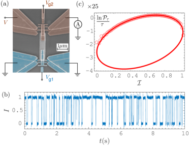
Figure 1: (color online). Experimental setup. (a) False-colored scanning electron micrograph of the SET (brown) and the SEB (blue). Both devices are fabricated by electron beam lithography and three-angle shadow evaporation Peltonen et al. (2015). The gate voltages $V_{\text{g1}}$ and $V_{\text{g2}}$ are used to control the tunneling rates. The bias voltage $V$ is applied across the SET and the current $I$ is measured. (b) The current in the SET switches between the two normalized values $\langle I_{-}\rangle\leavevmode\nobreak\ =0$ and $\langle I_{+}\rangle=1$ due to the tunneling of single electrons on and off the SEB. (c) Distribution of the time-integrated current ($\circ$) for the integration time $\tau=180$ ms together with the tilted ellipse given by Eq. (4). The controllable rates for tunneling on and off the SEB are $\Gamma_{+}=72$ Hz and $\Gamma_{-}=37$ Hz.

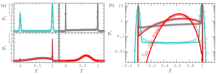
Figure 2: (color online). Distribution of the time-integrated current. (a) Experimental (circles) and theoretical (lines) results for the distribution $\mathcal{P}_{\tau}(\mathcal{I})$ with the integration times, $\tau=$ 4 ms (left top panel), 80 ms (right top panel), 320 ms (left bottom panel), and 1280 ms (right bottom panel). The tunneling rates are $\Gamma_{+}=130$ Hz and $\Gamma_{-}=70$ Hz. The theory curves are based on Eqs. (2,3) with no adjustable parameters. For short times, the distribution is bimodal with distinct peaks around the normalized currents $\langle I_{-}\rangle\leavevmode\nobreak\ =0$ and $\langle I_{+}\rangle=1$. At long times, the distribution is approximately normal-distributed around the mean $\langle I\rangle=\Gamma_{+}/(\Gamma_{+}+\Gamma_{-})\leavevmode\nobreak\ \simeq 0.65$. (b) The same results on a logarithmic scale.

Experimental setup.— Figure 1a shows an SET which is capacitively coupled to an SEB. Both are composed of small normal-conducting islands coupled to superconducting leads via insulating tunneling barriers. Measurements are performed at around 0.1 K, well below the charging energy of both the SEB and the SET. The tunneling rates of the SEB are tuned to the kilo-hertz regime so that the tunneling of electrons on and off the SEB are separated by milliseconds. The tunneling rates in the SET are on the order of several hundred megahertz and the electrical current is in the range of picoamperes. The conductance of the SET is highly sensitive to the presence of individual electrons on the SEB. This can be used to detect the individual tunneling events in the SEB by monitoring the current in the SET, see Fig. 1b Lu et al. (2003); Fujisawa et al. (2006); Gustavsson et al. (2006); Sukhorukov et al. (2007); Fricke et al. (2007); Gustavsson et al. (2009); Flindt et al. (2009); Ubbelohde et al. (2012); House et al. (2013); Maisi et al. (2014). Here, by contrast, we turn around these ideas and instead we focus on the current fluctuations in the SET under the influence of the random tunneling events in the SEB Hassler et al. (2011). This concept has an immediate application in characterization of spurious two-level fluctuators which appear in many solid-state devices Eiles et al. (1993); Paladino et al. (2014) and may affect the device properties. Thus, we use the SEB as an exemplary two-level fluctuator which can be completely characterized by considering the statistics of the current in the device in focus (the SET in our case).

Time-averaged current.— Our dynamical observable is the time-averaged current

$$\mathcal{I}(\tau)=\frac{1}{\tau}\int_{t_{0}}^{t_{0}+\tau}dtI(t)$$ (1)

measured over the time interval $[t_{0},t_{0}+\tau]$. For stationary processes, the distribution of current fluctuations depends only on the length of the interval $\tau$ and not on $t_{0}$. The distribution is expected to exhibit general properties that should be observable in any bistable conductor. For example, it has been predicted Jordan and Sukhorukov (2004) and verified in a related experiment Sukhorukov et al. (2007) that the logarithm of the distribution at long times is always given by a tilted ellipse, see Fig. 1c and Refs. Utsumi (2007); Lambert et al. (2015). Besides, the crossover from short to long times, see Fig. 2, gives additional information about the bistable system (SEB). This information can be used for the detection and characterization of parasitic two-level fluctuators that may be present in the vicinity of a device, since the fluctuation statistics should be universal for all such two-level systems as we will see.

Measurements.— Figure 2a shows experimental results for the distribution of the time-averaged current. For short integration times, the distribution is bimodal with two distinct peaks centered on the average currents $\langle I_{-}\rangle$ and $\langle I_{+}\rangle$ corresponding to having either $n=0$ or $n=1$ electrons on the SEB. According to the central limit theorem, the fluctuations should become normal-distributed with increasing integration time $\tau$, having a variance that decreases as $\mathcal{O}(\tau^{-1/2})$. This expectation is confirmed by Fig. 2a, showing how the distribution becomes increasingly peaked around the mean current $\langle I\rangle$. This behavior is similar to the suppression of energy or particle fluctuations in the ensemble theories of statistical mechanics Pathria and Beale (2011), here with the limit of long integration times playing the role of the thermodynamic limit. However, even as the distribution becomes increasingly peaked, rare fluctuations persist Touchette (2009). This can be visualized by using a logarithmic scale which emphasises the rare fluctuations encoded in the tails of the distribution, Fig. 2b. The rare fluctuations will be important when we below formulate and test a fluctuation theorem.

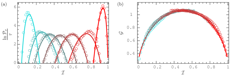
Figure 3: (color online). Tilted ellipse and and universal semi-circle. (a) Experimental (circles) and theoretical (lines) results for the logarithm of the distribution over the integration time, $\ln[\mathcal{P}_{\tau}(\mathcal{I})]/\tau$. The integration time is $\tau=400$ ms and the controllable tunneling rates $\Gamma_{+}/\Gamma_{-}$ are 40/315 Hz (turquoise), 109/248, 85/187, 88/98, 120/81, 166/55 and 285/20 (red) from left to right. The curves obtained from Eq. (4) include a finite-time off-set which is inversely proportional to $\tau$ sup . (b) When rescaled according to Eq. (5), the experimental data collapse onto the universal semi-circle indicated with a full red line.

Theory.— To better understand the fluctuations we develop a detailed theory of the distribution function $\mathcal{P}_{\tau}(\mathcal{I})$. The current fluctuates due to the random tunneling in the SEB and because of intrinsic noise in the SET itself. This we describe by the stochastic equation

$$\mathcal{I}(\tau)=[1-\mathcal{N}(\tau)]\langle I_{-}\rangle+\mathcal{N}(\tau)\langle I_{+}\rangle+\xi(\tau),$$ (2)

where the first two terms account for the random switching between the average currents $\langle I_{-}\rangle$ and $\langle I_{+}\rangle$ and we have defined the time-averaged electron number $\mathcal{N}(\tau)=\int_{t_{0}}^{t_{0}+\tau}dtn(t)/\tau$ on the SEB with $n=0,1$ Utsumi (2007). The time-averaged noise $\xi(\tau)$ describes the intrinsic fluctuations around the mean values $\langle I_{-}\rangle$ and $\langle I_{+}\rangle$, assumed here to be independent of $n$. The distribution of current fluctuations $\mathcal{P}_{\tau}(\mathcal{I})$ is now determined by the fluctuations of $\mathcal{N}(\tau)$ and the intrinsic noise $\xi(\tau)$. Electrons tunnel on and off the SEB with the tunneling rates $\Gamma_{+}$ and $\Gamma_{-}$, changing $n$ from 0 to 1 and vice versa, respectively. The distribution $\mathcal{P}_{\tau}(\mathcal{N})$ then becomes sup

$$\mathcal{P}_{\tau}(\mathcal{N})=\frac{e^{-[\Gamma_{+}(1-\mathcal{N})+\Gamma_{-}\mathcal{N}]\tau}}{\Gamma_{+}+\Gamma_{-}}\left\{\Gamma_{-}\delta\left(\mathcal{N}\right)+\Gamma_{+}\delta\left(1-\mathcal{N}\right)+2\tau\Gamma_{+}\Gamma_{-}\Pi(\mathcal{N})\left[I_{0}(x)+\tau[\Gamma_{-}(1-\mathcal{N})+\Gamma_{+}\mathcal{N}]\frac{I_{1}(x)}{x}\right]\right\}.$$ (3)

The boxcar function $\Pi(\mathcal{N})=\theta(\mathcal{N})\theta(1-\mathcal{N})$ is given by Heaviside step functions and $I_{0,1}(x)$ are modified Bessel functions of the first kind. We have also introduced the dimensionless parameter $x=2\tau\sqrt{\Gamma_{+}\Gamma_{-}\mathcal{N}(1-\mathcal{N})}$ controlling the distribution profile. For $\Gamma_{+}=\Gamma_{-}$, we recover the result of Ref. Bergli et al. (2009). Based on $\mathcal{P}_{\tau}(\mathcal{N})$, we can evaluate $\mathcal{P}_{\tau}(\mathcal{I})$ according to Eq. (2), taking into account the intrinsic fluctuations given by $\xi(\tau)$.

The resulting theory curves agree well with the experimental data in Fig. 2 over a wide range of integration times. For short times, $\tau\ll(\Gamma_{+}+\Gamma_{-})^{-1}$, we have $\mathcal{P}_{\tau}(\mathcal{N})\simeq[\Gamma_{-}\delta\left(\mathcal{N}\right)+\Gamma_{+}\delta\left(1-\mathcal{N}\right)]/(\Gamma_{+}+\Gamma_{-})$, corresponding to $\mathcal{P}_{\tau}(\mathcal{I})$ being bimodal with distinct peaks centered around the two average currents $\langle I_{-}\rangle$ and $\langle I_{+}\rangle$. With increasing integration time, the distribution eventually takes on the large-deviation form $\mathcal{P}_{\tau}(\mathcal{N})\propto e^{G(\mathcal{N})\tau}$ with the rate function $G(\mathcal{N})=-(\sqrt{\Gamma_{+}(1-\mathcal{N})}-\sqrt{\Gamma_{-}\mathcal{N}})^{2}$ following directly from Eq. (3). Moreover, the long-time limit of the distribution describes the low-frequency current fluctuations which should be dominated by the slow switching process. We can then ignore $\xi(\tau)$ in Eq. (2) such that the distribution becomes Jordan and Sukhorukov (2004)

$$\frac{\ln\mathcal{P}_{\tau}(\mathcal{I})}{\tau}\simeq-\frac{\left[\sqrt{\Gamma_{+}(\langle I_{+}\rangle-\mathcal{I})}-\sqrt{\Gamma_{-}(\mathcal{I}-\langle I_{-}\rangle)}\right]^{2}}{\langle I_{+}\rangle-\langle I_{-}\rangle}.$$ (4)

The rate function on the right-hand side characterizes the non-gaussian fluctuations of the current beyond what is described by the central limit theorem Touchette (2009). Importantly, the rate function is independent of the integration time and it captures the exponential decay of the probabilities to observe rare fluctuations. Geometrically, the rate function describes the upper part of a tilted ellipse, delimited by the currents $\langle I_{+}\rangle$ and $\langle I_{-}\rangle$ Jordan and Sukhorukov (2004); Sukhorukov et al. (2007); Utsumi (2007); Lambert et al. (2015). The tilt is given by the ratio of the controllable tunneling rates $\Gamma_{+}$ and $\Gamma_{-}$ and its width is governed by their product (see the prefactor in the parameter $x$). The tilted ellipse agrees well with the experimental results in the bistable range, $\langle I_{-}\rangle\leq\mathcal{I}\leq\langle I_{+}\rangle$, as seen in Fig. 1c. The extreme tails of the distribution are determined by the intrinsic fluctuations around $\langle I_{-}\rangle$ and $\langle I_{+}\rangle$ which are not included in Eq. (4).

By adjusting the tunneling rates we can control the shape and the tilt of the ellipse as illustrated in Fig. 3a. For $\Gamma_{-}\gg\Gamma_{+}$, the ellipse is strongly tilted to one side and the distribution is mostly centered around $\langle I_{-}\rangle$. As the ratio of the rates is changed, the ellipse becomes tilted to the other side and the distribution gets centered around $\langle I_{+}\rangle$. The average $\langle\mathcal{I}\rangle$ is given by the value of $\mathcal{I}$ where the distribution is maximal. This value changes from $\langle I_{-}\rangle$ to $\langle I_{+}\rangle$ as we tilt the ellipse. The abruptness of the change is determined by the width of the ellipse.

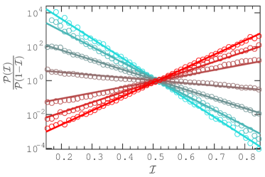
Figure 4: (color online). Experimental test of the fluctuation relation. With the two normalized average currents $\langle I_{+}\rangle=1$ and $\langle I_{-}\rangle=0$, Eq. (7) can be brought on the equivalent form $P_{\tau}(\mathcal{I})/P_{\tau}(1-\mathcal{I})=\exp[2\tau(\Gamma_{+}-\Gamma_{-})(\mathcal{I}-1/2)]$. In the figure, we plot the left-hand side using the experimental data ($\circ$) from Fig. 3, while the right-hand side is shown as full lines.

Universal semi-circle.— To provide a unified description of the fluctuations we define the rescaled distribution

$$\mathcal{G}(\mathcal{I})\equiv\frac{1}{2\sqrt{\Gamma_{+}\Gamma_{-}}}\left\{\frac{\ln\mathcal{P}_{\tau}(\mathcal{I})}{\tau}+\frac{\Gamma_{+}\Delta\mathcal{I}_{+}-\Gamma_{-}\Delta\mathcal{I}_{-}}{\langle I_{+}\rangle-\langle I_{-}\rangle}\right\},$$ (5)

where the second term in the brackets explicitly removes the tilt of the distribution and we have defined $\Delta\mathcal{I}_{\pm}=\mathcal{I}-\langle I_{\pm}\rangle$. From Eq. (4), we then obtain the semi-circle

$$\mathcal{G}^{2}(\mathcal{I})+\left(\frac{\mathcal{I}-\bar{I}}{\langle I_{+}\rangle-\langle I_{-}\rangle}\right)^{2}=1,$$ (6)

which should describe the fluctuations in any bistable conductor independently of the microscopic details. Here we have defined $\bar{I}=(\langle I_{+}\rangle+\langle I_{-}\rangle)/2$. Figure 3b shows that our experimental data in Fig. 3a measured at long times indeed collapse onto this semi-circle when rescaled according to Eq. (5). This property should hold for a variety of bistable systems from different fields of physics.

Fluctuation relation.— Finally, we examine the symmetry properties of the fluctuations Esposito et al. (2009). Equation (4) is suggestive of a fluctuation relation at long times reading

$$\frac{1}{\tau}\ln\left[\frac{P_{\tau}(\mathcal{I}=\bar{I}+\mathcal{J})}{P_{\tau}(\mathcal{I}=\bar{I}-\mathcal{J})}\right]=\Omega\mathcal{J},$$ (7)

where $\Omega=2(\Gamma_{+}-\Gamma_{-})/(\langle I_{+}\rangle-\langle I_{-}\rangle)$ controls the slope. This relation is reminiscent of the Gallavotti-Cohen fluctuation theorem Gallavotti and Cohen (1995a, b), however, here the intensive entropy production is replaced by the departure $\mathcal{J}$ from the average $\bar{I}$ of the mean currents. Equation (7) should be valid in the bistable region of the distribution which is dominated by the random tunneling in the SEB. The excellent agreement between theory and experiment in Fig. 4 confirms the prediction. The fluctuation relation is expected to be valid for many different bistable systems and may be further tested in future experiments.

Conclusions.— We have realized a controllable bistability in order to investigate fundamental properties of current fluctuations in bistable conductors. These include the cross-over from short-time to long-time statistics, the large-deviation principle, and the fluctuation relation in long-time limit. Our results have an immediate application for the detection and characterization of spurious two-level fluctuators which appear in many solid-state devices, since their fluctuations are universal and independent of the microscopic details. We have formulated and verified universal properties including a fluctuation relation for bistable conductors. Our work establishes several analogies between bistable conductors and concepts from statistical mechanics and it offers perspectives for further experiments on statistical physics with electronic conductors.

Acknowledgments.— We thank Yu. Galperin, F. Ritort, and K. Saito for useful discussions. The work was supported by Academy of Finland (projects 273827, 275167, and 284594) and Foundation Nanosciences under the aegis of Joseph Fourier University Foundation. We acknowledge the provision of facilities by Aalto University at OtaNano – Micronova Nanofabrication Centre. Authors at Aalto University are affiliated with Centre for Quantum Engineering.

See pages ,1 of supplement.pdf See pages ,2 of supplement.pdf See pages ,3 of supplement.pdf See pages ,4 of supplement.pdf

References

- Maruyama et al. (2009) K. Maruyama, F. Nori, and V. Vedral, “Colloquium: The physics of Maxwell’s demon and information,” Rev. Mod. Phys. 81, 1 (2009).
- Parrondo et al. (2015) J. M. R. Parrondo, J. M Horowitz, and T. Sagawa, “Thermodynamics of information,” Nat. Phys. 11, 131 (2015).
- Pekola (2015) J. P. Pekola, “Towards quantum thermodynamics in electronic circuits,” Nat. Phys. 11, 118 (2015).
- Koski et al. (2015) J. V. Koski, A. Kutvonen, I. M. Khaymovich, T. Ala-Nissila, and J. P. Pekola, “On-Chip Maxwell’s Demon as an Information-Powered Refrigerator,” Phys. Rev. Lett. 115, 260602 (2015).
- Chida et al. (2015) K. Chida, K. Nishiguchi, G. Yamahata, H. Tanaka, and A. Fujiwara, “Thermal-noise suppression in nano-scale Si field-effect transistors by feedback control based on single-electron detection,” Appl. Phys. Lett. 107, 073110 (2015).
- Koski et al. (2014) J. V. Koski, V. F. Maisi, J. P. Pekola, and D. V. Averin, “Experimental realization of a Szilard engine with a single electron,” Proc. Natl. Acad. Sci. USA 111, 13786 (2014).
- Toyabe et al. (2010) S. Toyabe, T. Sagawa, M. Ueda, E. Muneyuki, and M. Sano, “Experimental demonstration of information-to-energy conversion and validation of the generalized Jarzynski equality,” Nat. Phys. 6, 988 (2010).
- Bérut et al. (2012) A. Bérut, A. Arakelyan, A. Petrosyan, S. Ciliberto, R. Dillenschneider, and E. Lutz, “Experimental verification of Landauer’s principle linking information and thermodynamics,” Nature 483, 187 (2012).
- Jun et al. (2014) Y. Jun, M. Gavrilov, and J. Bechhoefer, “High-Precision Test of Landauer’s Principle in a Feedback Trap,” Phys. Rev. Lett. 113, 190601 (2014).
- Nakamura et al. (2010) S. Nakamura, Y. Yamauchi, M. Hashisaka, K. Chida, K. Kobayashi, T. Ono, R. Leturcq, K. Ensslin, K. Saito, Y. Utsumi, and A. C. Gossard, “Nonequilibrium Fluctuation Relations in a Quantum Coherent Conductor,” Phys. Rev. Lett. 104, 080602 (2010).
- Utsumi et al. (2010) Y. Utsumi, D. S. Golubev, M. Marthaler, K. Saito, T. Fujisawa, and G. Schön, “Bidirectional single-electron counting and the fluctuation theorem,” Phys. Rev. B 81, 125331 (2010).
- Küng et al. (2012) B. Küng, C. Rössler, M. Beck, M. Marthaler, D. S. Golubev, Y. Utsumi, T. Ihn, and K. Ensslin, “Irreversibility on the Level of Single-Electron Tunneling,” Phys. Rev. X 2, 011001 (2012).
- Saira et al. (2012) O.-P. Saira, Y. Yoon, T. Tanttu, M. Möttönen, D. V. Averin, and J. P. Pekola, “Test of the Jarzynski and Crooks Fluctuation Relations in an Electronic System,” Phys. Rev. Lett. 109, 180601 (2012).
- Koski et al. (2013) J. V. Koski, T. Sagawa, O.-P. Saira, Y. Yoon, A. Kutvonen, P. Solinas, M. Möttönen, T. Ala-Nissila, and J. P. Pekola, “Distribution of entropy production in a single-electron box,” Nat. Phys. 9, 644 (2013).
- Van Kampen (2007) N. G. Van Kampen, Stochastic Processes in Physics and Chemistry (Third Edition) (North Holland, 2007).
- Dieterich et al. (2015) E. Dieterich, J. Camunas-Soler, M. Ribezzi-Crivellari, U. Seifert, and F. Ritort, “Single-molecule measurement of the effective temperature in non-equilibrium steady states,” Nat. Phys. 11, 971 (2015).
- di Santo et al. (2016) S. di Santo, R. Burioni, A. Vezzani, and M. A. Muñoz, “Self-Organized Bistability Associated with First-Order Phase Transitions,” Phys. Rev. Lett. 116, 240601 (2016).
- Paladino et al. (2014) E. Paladino, Y. M. Galperin, G. Falci, and B. L. Altshuler, “ noise: Implications for solid-state quantum information,” Rev. Mod. Phys. 86, 361 (2014).
- Gustafsson et al. (2013) M. V. Gustafsson, A. Pourkabirian, G. Johansson, J. Clarke, and P. Delsing, “Thermal properties of charge noise sources,” Phys. Rev. B 88, 245410 (2013).
- Pourkabirian et al. (2014) A. Pourkabirian, M. V. Gustafsson, G. Johansson, J. Clarke, and P. Delsing, “Nonequilibrium Probing of Two-Level Charge Fluctuators Using the Step Response of a Single-Electron Transistor,” Phys. Rev. Lett. 113, 256801 (2014).
- Peltonen et al. (2015) J. T. Peltonen, V. F. Maisi, S. Singh, E. Mannila, and J. P. Pekola, “On-chip error counting for hybrid metallic single-electron turnstiles,” arXiv:1512.00374 (2015).
- Lu et al. (2003) W. Lu, Z. Q. Ji, L. Pfeiffer, K. W. West, and A. J. Rimberg, “Real-time detection of electron tunnelling in a quantum dot,” Nature 423, 422 (2003).
- Fujisawa et al. (2006) T. Fujisawa, T. Hayashi, R. Tomita, and Y. Hirayama, “Bidirectional counting of single electrons,” Science 312, 1634 (2006).
- Gustavsson et al. (2006) S. Gustavsson, R. Leturcq, B. Simovic, R. Schleser, T. Ihn, P. Studerus, K. Ensslin, D. C. Driscoll, and A. C. Gossard, “Counting Statistics of Single-Electron Transport in a Quantum Dot,” Phys. Rev. Lett. 96, 076605 (2006).
- Sukhorukov et al. (2007) E. V. Sukhorukov, A. N. Jordan, S. Gustavsson, R. Leturcq, T. Ihn, and K. Ensslin, “Conditional statistics of electron transport in interacting nanoscale conductors,” Nature Phys. 3, 243 (2007).
- Fricke et al. (2007) C. Fricke, F. Hohls, W. Wegscheider, and R. J. Haug, “Bimodal counting statistics in single-electron tunneling through a quantum dot,” Phys. Rev. B 76, 155307 (2007).
- Gustavsson et al. (2009) S. Gustavsson, R. Leturcq, M. Studer, I. Shorubalko, T. Ihn, K. Ensslin, D. C. Driscoll, and A. C. Gossard, “Electron counting in quantum dots,” Surf. Sci. Rep. 64, 191 (2009).
- Flindt et al. (2009) C. Fricke C. Flindt, F. Hohls, T. Novotný, K. Netočný, T. Brandes, and R. J. Haug, “Universal oscillations in counting statistics,” Proc. Natl. Acad. Sci. USA 106, 10116 (2009).
- Ubbelohde et al. (2012) N. Ubbelohde, C. Fricke, C. Flindt, F. Hohls, and R. J. Haug, “Measurement of finite-frequency current statistics in a single-electron transistor,” Nat. Commun. 3, 612 (2012).
- House et al. (2013) M. G. House, M. Xiao, G. Guo, H. Li, G. Cao, M. M. Rosenthal, and H. Jiang, “Detection and Measurement of Spin-Dependent Dynamics in Random Telegraph Signals,” Phys. Rev. Lett. 111, 126803 (2013).
- Maisi et al. (2014) V. F. Maisi, D. Kambly, C. Flindt, and J. P. Pekola, “Full Counting Statistics of Andreev Tunneling,” Phys. Rev. Lett. 112, 036801 (2014).
- Hassler et al. (2011) F. Hassler, G. B. Lesovik, and G. Blatter, “Influence of a random telegraph process on the transport through a point contact,” Eur. Phys. J. B 83, 349 (2011).
- Eiles et al. (1993) T. M. Eiles, J. M. Martinis, and M. H. Devoret, “Even-Odd Asymmetry of a Superconductor Revealed by the Coulomb Blockade of Andreev Reflection ,” Phys. Rev. Lett. 70, 1862 (1993).
- Jordan and Sukhorukov (2004) A. N. Jordan and E. V. Sukhorukov, “Transport Statistics of Bistable Systems,” Phys. Rev. Lett. 93, 260604 (2004).
- Utsumi (2007) Y. Utsumi, “Full counting statistics for the number of electrons in a quantum dot,” Phys. Rev. B 75, 035333 (2007).
- Lambert et al. (2015) N. Lambert, F. Nori, and C. Flindt, “Bistable Photon Emission from a Solid-State Single-Atom Laser,” Phys. Rev. Lett. 115, 216803 (2015).
- Pathria and Beale (2011) R. K. Pathria and P. D Beale, Statistical Mechanics (Butterworth-Heinemann, 2011).
- Touchette (2009) H. Touchette, “The large deviation approach to statistical mechanics,” Phys. Rep. 478, 1 (2009).
- (39) See the Supplemental Material for further details about these calculations.
- Bergli et al. (2009) J. Bergli, Yu. M. Galperin, and B. L. Altshuler, “Decoherence in qubits due to low-frequency noise,” New J. Phys. 11, 025002 (2009).
- Esposito et al. (2009) M. Esposito, U. Harbola, and S. Mukamel, “Nonequilibrium fluctuations, fluctuation theorems, and counting statistics in quantum systems,” Rev. Mod. Phys. 81, 1665 (2009).
- Gallavotti and Cohen (1995a) G. Gallavotti and E. G. D. Cohen, “Dynamical ensembles in stationary states,” J. Stat. Phys. 80, 931 (1995a).
- Gallavotti and Cohen (1995b) G. Gallavotti and E. G. D. Cohen, “Dynamical Ensembles in Nonequilibrium Statistical Mechanics,” Phys. Rev. Lett. 74, 2694 (1995b).