Catching jetted tidal disruption events early in millimetre

Abstract

Relativistic jets can form from at least some tidal disruption events (TDEs) of (sub-)stellar objects around supermassive black holes. We detect the millimeter (MM) emission of IGR J12580+0134 — the nearest TDE known in the galaxy NGC 4845 at the distance of only 17 Mpc, based on Planck all-sky survey data. The data show significant flux jumps after the event, followed by substantial declines, in all six high frequency Planck bands from 100 GHz to 857 GHz. We further show that the evolution of the MM flux densities are well consistent with our model prediction from an off-axis jet, as was initially suggested from radio and X-ray observations. This detection represents the second TDE with MM detections; the other is Sw J1644+57, an on-axis jetted TDE at redshift of 0.35. Using the on- and off-axis jet models developed for these two TDEs as templates, we estimate the detection potential of similar events with the Large Millimeter Telescope (LMT) and the Atacama Large Millimeter/submillimeter Array (ALMA). Assuming an exposure of one hour, we find that the LMT (ALMA) can detect jetted TDEs up to redshifts $z\sim 1$ (2), for a typical disrupted star mass of $\sim 1$ M_⊙. The detection rates of on- and off-axis TDEs can be as high as $\sim 0.6$ (13) and 10 (220) per year, respectively, for the LMT (ALMA). We briefly discuss how such observations, together with follow-up radio monitoring, may lead to major advances in understanding the jetted TDEs themselves and the ambient environment of the CNM.

1 Introduction

Supermassive black holes (SMBHs) are believed to be present at the nuclei of all major galaxies. While only a small fraction of these SMBHs are active, the properties of the silent majority could be revealed by observations of tidal disruption events (TDEs) — phenomena in which stars or sub-stellar objects are tidally disrupted when they pass close enough by SMBHs (e.g., Rees, 1988; Evans & Kochanek, 1989). Part of the debris of a disrupted object would be accreted onto the black hole, producing flaring X-ray and optical emission with a typical $t^{-5/3}$ light curve which traces the fallback rate of the stellar material (Phinney, 1989). TDEs are expected to occur every $10^{3}-10^{5}$ years for a typical galaxy (e.g., Magorrian & Tremaine, 1999; Wang & Merritt, 2004). This rate could be substantially enhanced (as high as once per a few years) in galaxy nuclei with binary SMBHs (e.g., Chen et al., 2009, 2011).

Energetic jets can be launched by a TDE. When they interact with the circum-nuclear medium (CNM), high energy particle acceleration occurs (e.g., Cheng, Chernyshov & Dogiel, 2006; Farrar & Gruzinov, 2009). Long-lasting, non-thermal radio emissions confirm that at least some TDEs did launch relativistic jets. This catalogue includes Sw J1644+57 (Bloom et al., 2011; Burrows et al., 2011; Zauderer et al., 2011; Berger et al., 2012; Zauderer et al., 2013), Sw J2058+05 (Cenko et al., 2012), Sw J1112-82 (Brown et al., 2015), IGR J12580+0134 (Nikołajuk & Walter, 2013; Irwin et al., 2015), and possibly ASASSN-14li (van Velzen et al., 2016). The fraction of jetted TDEs is yet unclear. Bower et al. (2013) searched for the late-time radio emission from seven X-ray selected TDEs and found that two of them might have radio counterparts, which implied that $\lower 2.0pt\hbox{$\,\buildrel\scriptstyle>\over{\scriptstyle\sim}\,$}10\%$ of the X-ray-detected TDEs might have launched relativistic jets. However, van Velzen et al. (2013) observed seven other TDE candidates, all of which triggered within 10 years, but found that none of them had radio emission up to $10\,\mu$Jy level, although most of these sources are relatively distant ($z\approx 0.14-0.37$). At present, the number statistics is too small to allow for a reliable estimate of the jetted fraction. Enlarging the jetted TDE sample is thus crucial to the understanding of the jet formation (e.g., its dependence on SMBH spins; Lei & Zhang 2011).

TDE jets also provide unique diagnostics of the environment around SMBHs. The jet emission reveals the CNM density and/or magnetic field (producing Faraday rotation) profiles on sub-parsec scales, which can hardly be probed in any other ways. Unlike $\gamma$-ray bursts (GRBs) whose time scales are typically of the order of hours to days for afterglows, the corresponding observable time scales of TDEs are of the order of months to years. A long time scale allows for easy follow-up of such events, especially for the early development of jets. Furthermore, the spatial scales of TDEs are also large enough, allowing for spatially-resolved studies for some nearby events (e.g., IGR J12580+0134 at $d\approx 17$ Mpc).

Timely follow-up observations of TDE jets are very important for probing their early evolution. However, early follow-ups are strongly affected by the self-absorption of synchrotron emission in radio (Irwin et al., 2015). The infrared and optical emission from jets is typically not expected to be bright and could suffer serious confusion from galactic emission and/or extinction of the interstellar medium, especially in the nuclear regions of the host galaxies. Observing TDEs in (sub-)millimeter (MM) is thus optimal for detecting the jets in the earliest stages. As the jets expand in the CNM, the emission gradually becomes optically thin, first at high frequencies and eventually down to the radio. A complete view of the jet evolution from its earliest stages can potentially allow us to understand the overall energetics of the jets, the CNM environment, as well as the high energy particle acceleration. In this work we assess this potential of observing TDE candidates (which are supposed to be discovered typically in X-ray and optical surveys) with the MM facilities such as the Large Millimeter Telescope Alfonso Serrano (LMT) and the Atacama Large Millimeter Array (ALMA), in addition to the presentation of our data analysis results based on the existing Planck all-sky survey.

This paper is organized as follows. In § 2, after a brief introduction on the current MM observations of TDEs, we present an analysis of the Planck data on IGR J12580+0134. Taking Sw J1644+57 and IGR J12580+0134 as the templates of on- and off-axis jetted TDEs, we describe the modeling of the emission from TDE jets in § 3. In § 4 we study the detectability and event rates of jetted TDEs with the LMT and ALMA. We discuss possible physical insights of MM observations on TDEs and related topics in § 5, and finally summarize our work in § 6.

2 MM detections of TDEs with existing observations

Up to now there are about 60 candidates of TDEs, most of which were discovered in X-ray and optical. A few of them were long-lasting radio sources, suggesting the scenario of synchrotron emission from non-thermal electrons accelerated at the jet-induced shocks in the CNM. In the MM bands, only Sw J1644+57 ($z=0.35$) was detected with the Combined Array for Research in Millimeter Astronomy (CARMA) at 87 GHz and the Submillimeter Array (SMA) at 200, 230 and 345 GHz (Berger et al., 2012). The MM emission peaks at $t\lower 2.0pt\hbox{$\,\buildrel\scriptstyle<\over{\scriptstyle\sim}\,$}10$ days after the outburst of the TDE and has a flux $\sim 20$ mJy at 87 GHz (Berger et al., 2012). The combined MM and radio observations extending to $\sim 200$ days show clearly two components of the light curves (see § 3.1 and Fig. 2), indicating that the jet is structured (Berger et al., 2012; Wang et al., 2014; Liu, Pe’er & Loeb, 2015).

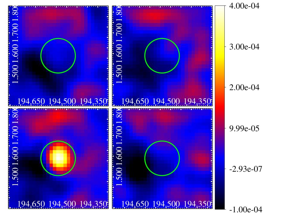
Figure 1: Left panel: $30^{\prime}\times 30^{\prime}$ minimaps (smoothed with a Gaussian kernel with $\sigma=2^{\prime}$) of Planck observations of NGC 4845 at 217 GHz, at $T_{1}$ (top-left), $T_{2}$ (top-right), $T_{3}$ (top-left), and $T_{4}$ (top-right). The green circle outlines a $10^{\prime}$ diameter region centered at NGC 4845 in each sub-panel. The units of the colorbar are ${\rm K_{CMB}}$. Right panel: the four epoch flux densities of NGC 4845 at the 353 (top), 545 (middle), and 857 (bottom) GHz frequencies. The dashed line in each sub-panel shows the average flux densities of the first two epochs, which represents the emission of the galaxy.

Table 1: Flux densities of the Planck observations of NGC 4845.

$\nu$	2010-01-16 ($T_{1}$)	2010-07-05 ($T_{2}$)	2011-01-16 ($T_{3}$)	2011-07-05 ($T_{4}$)	TDE at $T_{3}$
(GHz)	(mJy)	(mJy)	(mJy)	(mJy)	(mJy)
30	—	—	—	—	$<427^{a}$
44	—	—	—	—	$<692^{a}$
70	—	—	—	—	$<501^{a}$
100	—	—	$640\pm 103$	—	$635\pm 103^{b}$
143	—	—	$741\pm 37$	—	$726\pm 37^{b}$
217	—	—	$675\pm 42$	—	$615\pm 42^{b}$
353	$275\pm 96$	$274\pm 79$	$693\pm 87$	$396\pm 88$	$419\pm 107^{c}$
545	$1307\pm 114$	$1293\pm 122$	$1756\pm 117$	$1236\pm 142$	$456\pm 144^{c}$
857	$5846\pm 120$	$5668\pm 111$	$6336\pm 117$	$5573\pm 120$	$579\pm 143^{c}$

Notes: ^aMinimum flux density at $90\%$ completeness (Planck Collaboration et al., 2015). ^bFlux density of IGR J12580+0134 at $T_{3}$ after subtracting the emission of the galaxy which is assumed to follow the power-law extrapolation of those (mean of $T_{1}$ and $T_{2}$) at 353, 545, and 857 GHz. ^cInferred flux density of IGR J12580+0134 at $T_{3}$ after subtracting the mean emission of $T_{1}$ and $T_{2}$.

We note that Planck surveyed the MM sky for 8 times with the low frequency instrument (LFI; at 30, 44, and 70 GHz) and 5 times with the high frequency instrument (HFI; at 100, 143, 217, 353, 545, and 857 GHz) during its four years’ operation. Two Planck catalogues of compact sources (PCCS), with the first one (PCCS1) covering the period from August 12, 2009 to November 27, 2010, and PCCS2 covering from August 12, 2009 to January 11, 2012 (for the HFI), have been released by the Planck team (Planck Collaboration et al., 2014, 2015). We thus conduct a search for potential counterparts for the TDE candidates which were detected from the beginning of 2009 to the end of 2011 in the PCCS1 and PCCS2 catalogues. About 20 TDE candidates are searched, and we find a counterpart of the TDE IGR J12580+0134, discovered by INTEGRAL (Nikołajuk & Walter, 2013) in December, 2010, in the nearby galaxy NGC 4845. This counterpart is represented by a variable source positionally coincident (within the beam full widths at half maximum (FWHM), which are $\sim 5-10^{\prime}$ for the HFI; Planck Collaboration et al. 2014) with IGR J12580+0134. The fluxes seen in PCCS2 are systematically higher than those in PCCS1, suggesting the emission from the TDE.

To quantify the MM emission of the TDE, we have systematically analyzed the Planck survey data. Table 1 summarizes the detected emission in the four epochs covered by the HFI. The left-hand panel of Fig. 1 shows our extracted 217 GHz minimaps centered at NGC 4845 for these four epochs. These maps have been smoothed with a Gaussian kernel with $\sigma$ of 2’. A substantial brightening at the source location can be seen at $T_{3}$ (bottom-left sub-panel), just after the outburst of the TDE. We estimate the flux density of the source in the raw imaging data of each map using a Gaussian fit photometry method (Planck Collaboration et al., 2014, 2015). Since the galaxy is unresolved by Planck, we employ a symmetric Gaussian function with width $\sigma$ fixed at FWHM/2.355, plus a constant background, to fit the image. The FWHM values of each image is adopted from Planck Collaboration et al. (2014). The normalization of the noise is obtained by setting the best-fit reduced $\chi^{2}=1$, and the uncertainty of the flux density is computed from the curvature of the $\chi^{2}$ (Planck Collaboration et al., 2014, 2015). The results are given in Table 1. No significant source is found in the LFI observations, and the minimum flux densities corresponding to $90\%$ completeness of the PCCS2 catalogue are given. For the HFI bands, the galaxy is detected at all four epochs at 353, 545, and 857 GHz. The flux densities in these three bands are shown in the right-hand panel of Fig. 1, as well as in Table 1. We see that the flux densities of the galaxy increase significantly at $T_{3}$ for all three bands, compared to those at $T_{1}$ and $T_{2}$. The emission droped to the average level at $T_{4}$, except for the 353 GHz band which was still brighter than the average. Taking the mean flux densities of $T_{1}$ and $T_{2}$ as the emission of the galaxy, we can derive the flux densities of TDE IGR J12580+0134 at $T_{3}$, which are given by the last column of Table 1. For the 100, 143, and 217 GHz bands, the emission is detected only at $T_{3}$. The flux densities of the TDE are then derived through subtracting the extrapolated galaxy emission assuming a power-law spectrum according to the higher frequency results (mean of that of $T_{1}$ and $T_{2}$).

3 Models for jetted TDEs

Here we provide an overview of the afterglow emission modeling of jetted TDEs. Taking Sw J1644+57 and IGR J12580+0134 as examples of on- and off-axis jetted TDEs, we demonstrate the modeling of the multi-band and multi-epoch data. The model is somehow simple, with one-dimensional (radial) evolution of the jets. The two-dimensional model with the lateral expansion (Mimica et al., 2015; Generozov et al., 2016) would describe the jet dynamics more precisely. However, for the purpose of this work and/or the data quality for these objects, the one-dimensional model is expected to be adequate.

3.1 On-axis TDEs

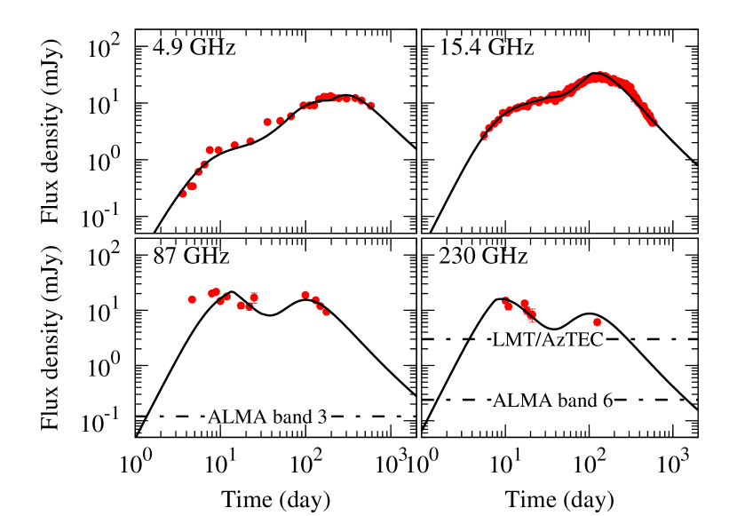
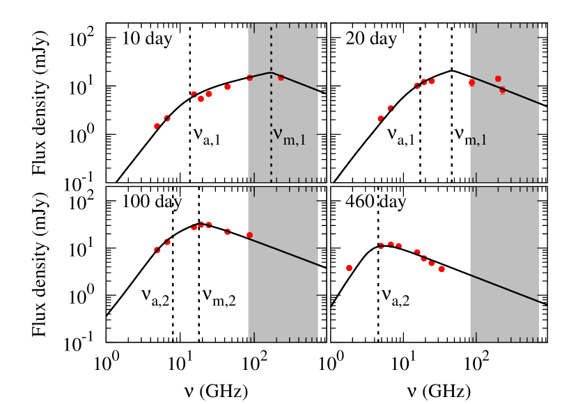
Figure 2: Left: light curves of the on-axis TDE Sw J1644+57 at 4.9, 15.4, 87, and 230 GHz, respectively. The solid lines show the predictions of the two-component jet model (Wang et al., 2014), compared with the observational data (Berger et al., 2012; Zauderer et al., 2013). Horizontal lines show the sensitivities of the LMT and ALMA at different bands (Table 3). Right: SEDs of Sw J1644+57 at 10, 20, 100, and 460 day, respectively. Vertical dotted lines represent the typical frequencies $\nu_{a}$ (the self-absorption frequency) and $\nu_{m}$ (the frequency corresponding to the minimum injection energy of electrons). The subscription “1” (“2”) refers to the inner-fast (outer-slow) jet which dominates the emission at early (late) stages.

Table 2: Model parameters from the radio data fitting

	$\Delta t$ (day)	$n_{18}$ (${\rm cm}^{-3}$)	$k$	$\theta_{\rm obs}$ (deg)	$E_{50}^{a}$	$\Gamma_{j}$	$\theta_{j}$ (deg)	$p$	$\epsilon_{e}^{b}$	$\epsilon_{B}^{b}$
Sw J1644+57 (inner)	0.25c	0.05	0.0	1.4	9000	8.7	1.7	2.20	0.13	0.13
Sw J1644+57 (outer)	0.25c	0.05	0.0	1.4	9000	3.6	4.5	2.20	0.25	0.31
IGR J12580+0134	30d	8.8	—	35	72	4.6	9.5	1.80	0.25	0.25

Notes: Columns from left to right are: source name, jet launching time, CNM density at $10^{18}$ cm, power-law index of the density profile, viewing angle, kinetic energy of the jet, initial Lorentz factor of the jet, opening angle of the jet, spectral index of accelerated electrons, electron energy density fraction, and magnetic field energy density fraction.

^aIn $10^{50}$ erg s^-1. ^bFraction of the ejecta kinetic energy assigning to accelerated electrons or the magnetic field. ^cRelative to March 25.5, 2011. ^dRelative to December 12, 2010.

The physical picture of on-axis jetted TDEs is similar to that of GRBs. The central engine, the tidal disruption of stellar objects by SMBHs, powers relativistic jets, which then propagate in the CNM. The internal dissipation within the jets, probably together with emission from the accretion disk and/or its corona, could be responsible for the early X-ray/UV/optical emission, which corresponds to the prompt emission of GRBs. The jet-CNM interaction generates shocks to accelerate electrons (or even cosmic rays) which radiate via synchrotron and/or inverse Compton scattering, giving rise to the so-called afterglow emission. The evolution of a jet during the propagation in the CNM includes roughly three stages. The jet first undergoes a coasting phase with a nearly constant speed. Then it starts to decelerate when the mass of the CNM swept by the forward shock is comparable to $M_{\rm ej}/\Gamma_{j}$, where $\Gamma_{j}$ and $M_{\rm ej}$ are the initial Lorentz factor and mass of the ejecta. Finally the blastwave enters the Newtonian phase when the rest mass equivalent energy of the swept CNM is comparable to the initial kinetic energy of the jets. The dynamics of the jet may then be described by a set of hydrodynamical equations (Huang et al., 2000). We here adopt a numerical approach to describe the jet dynamics, and follows Sari, Piran & Narayan (1998) (see Gao et al. 2013 for a more comprehensive version) to calculate the synchrotron emission from the accelerated electrons. We have a total of 10 parameters to describe the jet dynamics, radiation, and the CNM density structure, as shown in Table 2.

A two-component jet model has been developed by Wang et al. (2014), to explain the complex multi-wavelength light curves of Sw J1644+57. We use a similar but improved version of the model to fit the multi-wavelength and multi-epoch data (Berger et al., 2012; Zauderer et al., 2013). Instead of a constant density of the CNM, we assume a power-law distribution $n(r)=n_{\rm 18}(r/{10^{18}\,{\rm cm}})^{-k}$. Furthermore, we introduce an additional parameter $\Delta t$, after the outburst of the event, to characterize the zero point of the jet evolution. Fig. 2 shows the model light curves (left) and the spectral energy distributions (SED; right) that fit the observational data. The two bumps in the light curves (left-hand panels of Fig. 2) represent the contributions from the inner-fast and the outer-slow jets, which dominate the emission at early and late stages, respectively. We find a small difference (with $\Delta t=0.25$ days) of the jet launching time relative to the $\gamma$-ray outburst time of Sw J1644+57, March 25.5, 2011 (Zauderer et al., 2011). The fitting suggests $k\sim 0$, indicating that the jets propagate in a uniform, low density environment. However, we note from Fig. 2 that this model does not reproduce the light curves and SEDs well enough. Further refinement of the model is necessary, possibly including the spectral evolution of accelerated electrons.

The model parameters are given in Table 2. These parameters are somewhat different from those in Wang et al. (2014), because of the likelihood fitting technique adopted in this work. Note, however, these parameters are only a set of representative ones which can describe the data, because of strong degeneracies of the model parameters. A quantitative assessment of the confidence regions of the parameters is non-trivial due to the systematic uncertainties of the radio observations (from e.g., calibration and scintillation), and beyond the purpose of this study. Furthermore, the model parameters from the two-dimensional model are expected to be different from those from the one-dimensional one adopted here (Mimica et al., 2015).

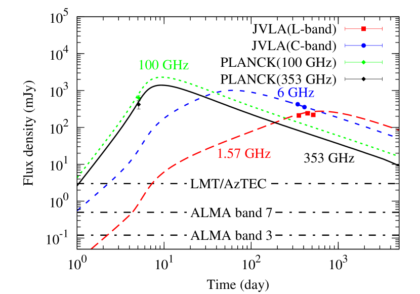
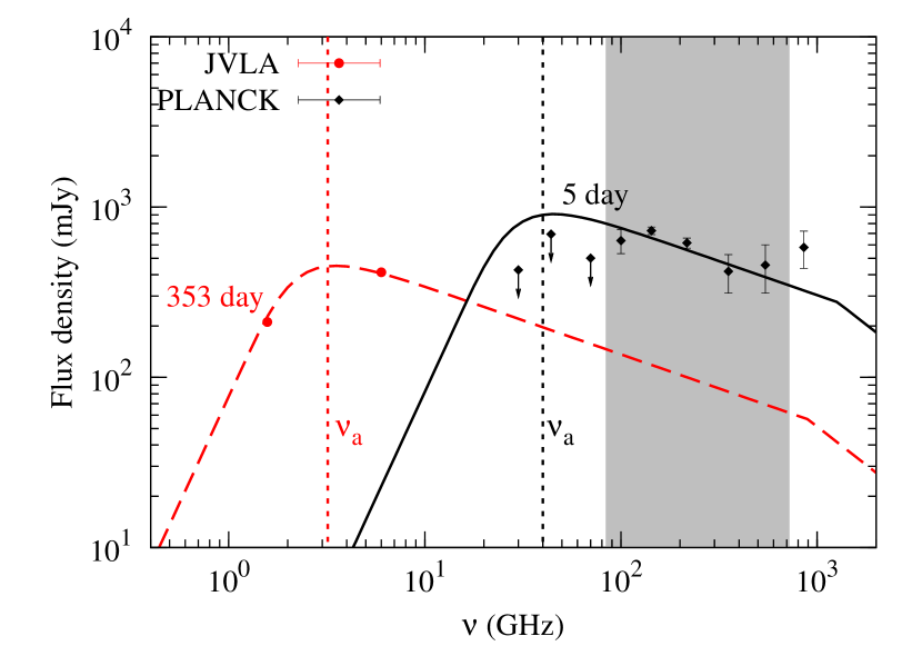
Figure 3: Left: model light curves of the off-axis TDE IGR J12580+0134 at 1.57, 6, 100, and 353 GHz. Right: SED of IGR J12580+0134 at 5 and 353 days. The radio data are from Irwin et al. (2015), and the MM data are from Planck analyzed in this work. Lines show the fitting results of the jet-CNM interaction model.

3.2 Off-axis TDEs

A TDE seen off-axis should be substantially less luminous than if observed on-axis, due to the lack of significant Doppler boosting. The ratio of the off-axis to on-axis Doppler factors is (Granot et al., 2002)

$$a_{\rm off}=\frac{{\mathcal{D}}_{\rm off}}{{\mathcal{D}}_{\rm on}}=\frac{1-\beta}{1-\beta\cos\psi},$$ (1)

where $\beta$ is the velocity of a jet in units of the light speed $c$, and $\psi=\max(\theta_{\rm obs}-\theta_{j},\,0)$ is the angle between the jet moving direction and the LOS. The bolometric luminosity scales as $L^{\rm off}\sim a_{\rm off}^{4}L^{\rm on}$. Typically for $\Gamma\sim$ a few (e.g., 4) and $\psi\sim\pi/4$, we have $a_{\rm off}\sim 0.1$. The factor $a_{\rm off}$ mainly takes effects at early time when the jet is relativistic. With the deceleration of the jet, $a_{\rm off}$ approaches 1 asymptotically, and the difference between on- and off-axis viewing angles becomes smaller. This can explain the $\sim 7000$ times difference of the X-ray luminosities (after correcting the mass difference of the disrupted objects) between Sw J1644+57 and IGR J12580+0134 (Lei et al., 2016). The late time (e.g., $t\sim 100$ day) radio luminosities of these two events, after correcting the mass difference of the disrupted objects, are comparable with each other when no significant effect from $a_{\rm off}$ applies.

The same model for on-axis TDEs can be applied to off-axis ones, with proper modifications of the viewing angle effect, e.g., $\nu^{\rm off}=a_{\rm off}\nu^{\rm on}$, $t^{\rm off}=t^{\rm on}/a_{\rm off}$, $F_{\nu}^{\rm off}(t)=a_{\rm off}^{3}F_{\nu/a_{\rm off}}^{\rm on}(a_{\rm off}\,t)$. Since the data of IGR J12580+0134 are not good enough to constrain the CNM density profile, we assume a constant density here. Fig. 3 shows the light curves (left) and SEDs (right) for the model fitting results, compared with the radio data by the Jansky Very Large Array (JVLA; Irwin et al., 2015) and the Planck data obtained in § 2. It is shown that the Planck HFI data are reasonably consistent with the model at early time of the outburst. However, the Planck LFI data may suggest a harder spectrum than that inferred from the JVLA data, which implies a possible spectral evolution of accelerated electrons in the TDE jets. The non-detection of the source in the Planck LFI data may also partly be due to the optical thickness of the emission at the early time. We further find that the zero point of the jet launching is about 30 days after the first X-ray detection on December 12, 2010 and about 12 days before the X-ray peak time (Nikołajuk & Walter, 2013), which suggests a non-jet origin of the X-ray emission (see also Lei et al., 2016).

Still the model parameters, shown in Table 2, just represent one potential combination which can describe the data. The one-dimensional model may also lead to differences compared with the two-dimensional case (Mimica et al., 2015). This is more severe for IGR J12580+0134 than that of Sw J1644+57, because the model is less constrained by the limited data points. Since larger uncertainties of the emission of off-axis jetted TDEs may come from the scaling of $a_{\rm off}$ factor and the mass of the disrupted object (about $10^{2}$ times smaller for IGR J12580+0134 than a typical star; Nikołajuk & Walter, 2013), we do not explore more detailed and complicated modeling in this work, but take a few different scaling relations between $L^{\rm off}$ and $L^{\rm on}$ to account for potential uncertainties instead.

4 Potential capabilities of existing MM observing facilities

4.1 Facilities

We take the LMT and ALMA as representives of single-dish telescopes and telescope arrays for the discussion. Other facilities such as the James Clerk Maxwell telescope (JCMT), SMA, and CARMA, are expected to be within the capability ranges of the LMT and ALMA. The LMT and ALMA, with latitudes $19^{\circ}$N and $23^{\circ}$S, respectively, will cover the northern and southern sky complimentarily. Furthermore, a single-dish telescope may be sufficient to observe a relatively bright source and more flexible for a quick check of an event’s brightness, as well as for potential subsequent monitoring, while the telescope array may be well suitable for detecting faint sources and for high-resolution imaging of some nearby sources to resolve the jet structures.

4.1.1 LMT

The LMT is a single-dish MM telescope, located on the summit of Volcan Sierra Negra, Mexico at an altitude of 4600 m above the sea level (Hughes et al., 2010). It is designed for astronomical observations in the wavelength range of $0.85-4$ mm. The LMT is currently operating with the finished 32-meter diameter aperture and will soon have the full 50-meter diameter. The corresponding angular resolution is $\sim 8^{\prime\prime}$ currently (will finally be $\sim 5^{\prime\prime}$), and the pointing accuracy is $\sim 1^{\prime\prime}$. The two commissioned instruments are the Redshift Search Receiver (RSR), a wide-band 3 mm spectrometer, and the Astronomical Thermal Emission Camera (AzTEC), a 1.1 mm continuum camera. The sensitivity of the AzTEC instrument is about $0.6$ mJy root-mean-square (RMS) for an hour exposure under the small map mode, which is designed to map a 1.5 arcmin diameter region with uniform sensitivity (see Table 3).

4.1.2 ALMA

The ALMA is located at the Atacama desert in Chile with an altitude of about 5000 meters above the sea level. The dryness and high altitude makes Atacama well suited for MM observations. The ALMA is a telescope array consisting of 66 antennas when completed, 54 of them with 12-meter diameter dishes and 12 smaller ones with 7-meter diameter. After the full installation, the ALMA will cover 10 frequency bands of the (sub-)MM windows from $\sim 30$ GHz (10 mm) to THz (0.3 mm). Currently the ALMA operates in part as the Early Science phase, with more than sixteen 12-meter antennas, yielding sensitivites of $\sim 10\%$ of the full array. The bands 3, 6, 7 and 9 are available, covering frequencies from 84 GHz to 720 GHz (see Table 3). The maximum baseline is about 250 m, resulting in a maximum angular resolution of $\sim 2.5^{\prime\prime}$ in band 3 and $0.4^{\prime\prime}$ in band 9. The continuum sensitivity is about $0.1-3.6$ mJy, for an hour exposure and a $5\sigma$ significance, as shown in Table 3 (de Ugarte Postigo et al., 2012).

Table 3: Typical (sub-)MM observational bands and sensitivities

	$\nu$	$\lambda$	sensitivitya
	(GHz)	(mm)	(mJy)
LMT/AzTEC	273	1.1	3.0b
ALMA band 3	$84-116$	$2.58-3.56$	0.12c
ALMA band 6	$211-275$	$1.09-1.42$	0.24c
ALMA band 7	$275-373$	$0.80-1.09$	0.50c
ALMA band 9	$602-720$	$0.42-0.50$	3.60c

Notes: ^aThe sensitivity is defined as 5 times of the achievable RMS for 1-hour observations. ^bhttp://www.lmtgtm.org/?page_id=713 . ^cFor the early science operation of the ALMA (de Ugarte Postigo et al., 2012).

4.2 Detectability

Figs. 2 and 3 compare the sensitivities of the LMT and ALMA to the detected/expected fluxes of Sw J1644+57 and IGR J12580+0134. Both sources were bright enough to be detectable at their peak time by the LMT and ALMA, and could still be detectable years (for the LMT) or even ten years (for the ALMA) after their outbursts. Note, however, the contamination from the galactic nuclei may be important for an observation at a late stage when the flux has decreased significantly, especially for a single-dish telescope. Considering the peak fluxes, we find that the LMT (ALMA) can detect Sw J1644+57-like events up to redshifts of $z\sim 0.8$ (2.4), and IGR J12580+0134-like events up to $z\sim 0.1$ (0.35). If the disrupted object mass of an IGR J12580+0134-like event is as massive as an ordinary star ($\sim$M_⊙), such off-axis TDEs could be detectable up to $z\sim 0.7$ (2.2).

The wavelength coverages of the LMT and ALMA are shown with shaded regions in the right-hand panels of Figs. 2 and 3. While the low frequency spectra are modifided by the self-absorption and the minimum energy of accelerated electrons, the (sub-)MM observations are weakly affected by these effects, and hence can directly measure the spectral index of electrons. The MM emission in the early time may also trace the evolution of $\nu_{m}$, which is helpful to understanding the acceleration of electrons in the shocks.

4.3 Detection rate

The event rate density of Sw J1644+57-like (on-axis) jetted TDEs can be estimated as (Sun, Zhang & Li, 2015)

$$\rho^{\rm on}(L^{\rm on}_{p,{\rm bol}},z)=\frac{\rho^{\rm on}_{0}}{L_{0}^{\rm on}}\left(\frac{L^{\rm on}_{p,{\rm bol}}}{L_{0}^{\rm on}}\right)^{-2.0}\times f(z),$$ (2)

where $L^{\rm on}_{p,{\rm bol}}$ is the peak bolometric luminosity in the rest-frame $1-10^{4}$ keV range, $\rho_{0}\approx 0.03$ Gpc^-3 yr^-1 is the local event rate density for source luminosities above $L_{0}^{\rm on}=10^{48}$ erg s^-1, and $f(z)$ gives the redshift dependence of TDEs based on the semi-empirical models of the SMBH mass density distribution (Shankar, Weinberg & Miralda-Escudé, 2013; Sun, Zhang & Li, 2015)

$$f(z)=\left[(1+z)^{0.2\eta}+\left(\frac{1+z}{1.43}\right)^{-3.2\eta}+\left(\frac{1+z}{2.66}\right)^{-7.0\eta}\right]^{1/\eta},$$ (3)

with $\eta=-2$.

We generalize Eq. (2) to include off-axis jetted TDEs as

$$\rho(L^{\rm off},z)=\epsilon^{-1}\times\rho^{\rm on}(L^{\rm on},z)\cdot\frac{dL^{\rm on}}{dL^{\rm off}},$$ (4)

where we have ignored the subscript “$p,{\rm bol}$” of the luminosity and $\epsilon=(1-\cos\theta_{j})/(1-\cos\theta_{\rm obs}^{\rm max})$ is the sky coverage fraction of the jets. In this work we assume $\theta_{j}\sim 15^{\circ}$. By definition we have $\theta_{\rm obs}^{\rm max}=\theta_{j}$ (hence $\epsilon^{-1}=1$) for on-axis sources, and $\theta_{\rm obs}^{\rm max}=\pi/2$ (hence $\epsilon^{-1}\sim 30$) for off-axis sources. For on-axis TDEs, $a_{\rm off}=1$, Eq. (4) recovers Eq. (2). More generally Eq. (4) should be averaged over $a_{\rm off}$ which is a function of the viewing angle $\theta_{\rm obs}$ and the Lorentz factor $\Gamma$. Because there are no good constraints on the distribution of $\Gamma$, and hence $a_{\rm off}$, we assume a typical value of $a_{\rm off}=0.1$ for the discussion of off-axis sources except in Table 4 where other values of $a_{\rm off}$ are considered additionally. Fixing the value of $a_{\rm off}$ also makes it possible to estimate the detectability of off-axis TDEs by MM facilities by re-scaling the template source, IGR J12580+0134. However, one should keep in mind that this assumption may be an over-simplification.

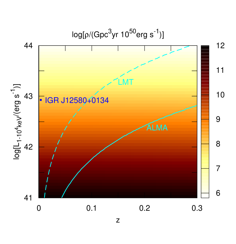
Figure 4: Event rate density $\rho(L,z)$ of on-axis (left) and off-axis (right; $a_{\rm off}^{4}=10^{-4}$) jetted TDEs as a function of redshift and $1-10^{4}$ keV bolometric luminosity. Curves show the sensitivities of the LMT and ALMA, above which TDEs are detectable, assuming that they can be characterized by the models of energetical scaling of Sw J1644+57 (for the on-axis type) or IGR J12580+0134 (for the off-axis type).

Given a specific detection threshold, the detectable event rate is obtained through integrating the event rate density over the luminosity and the cosmological volume (Sun, Zhang & Li, 2015)

$$\frac{dN}{dt}=\frac{\Omega}{4\pi}\int dL\int_{0}^{z_{\rm max}(L)}dz\,\frac{\rho(L,z)}{1+z}\frac{dV}{dz},$$ (5)

where

$$\frac{dV}{dz}=\frac{c}{H_{0}}\frac{4\pi d_{L}^{2}}{(1+z)^{2}[\Omega_{M}(1+z)^{3}+\Omega_{\Lambda}]^{1/2}}$$ (6)

is the cosmological specific comoving volume (assuming the standard $\Lambda$CDM cosmology) with $d_{L}$ the luminosity distance, $\Omega/4\pi$ is the fraction of the sky covered by the instrument, and $z_{\rm max}(L)$ is the maximum redshift that a source with luminosity $L$ can be detected. In this work we assume $\Omega/4\pi\approx 1/2$ for both the LMT and the ALMA. The maximum redshift can be obtained through a scaling of the template source as

$$d_{L}^{2}(z_{\rm max}(L))=d_{L}^{2}(z_{\rm ref})\times L/(L_{\rm ref}/k),$$ (7)

where $k$ is the ratio of the reference source flux to the detector sensitivity (see Table 3).

Table 4: Number of TDEs per year above MM detection thresholds

	LMT/AzTEC	ALMA
On-axis	0.6	10
Off-axis ($a_{\rm off}^{4}=10^{-4}$)	13	220
Off-axis ($a_{\rm off}^{4}=10^{-3}$)	130	2230
Off-axis ($a_{\rm off}^{4}=10^{-5}$)	1.3	22

Fig. 4 shows the event rate density as a function of the peak bolometric luminosity and redshift, for on-axis (left) and off-axis (right) jetted TDEs, respectively. The curves overplotted show the MM detection threshold (or $z_{\rm max}$ for a given $L$) above which the sources are detectable, assuming the same peak bolometric luminosity to peak MM flux ratio of Sw J1644+57 (IGR J12580+0134) for on-axis (off-axis) sources. Integrating the regions above the curves shown in Fig. 4 gives the event rate, as listed in Table 4. In reality, one also needs to account for the trigger efficiency of TDEs (Khabibullin, Sazonov & Sunyaev, 2014; Donnarumma & Rossi, 2015), as well as the visibility by the MM telescopes.

Figure 5: Luminosity distribution $L\times g(L)$ of detectable TDEs as defined in Eq. (8). Solid and dashed lines are for on-axis and off-axis ($a_{\rm off}^{4}=10^{-4}$) TDEs, respectively. For each type, the higher one is for the ALMA, and the lower one is for the LMT.

We define the redshift integral part of Eq. (5) as

$$g(L)=\frac{\Omega}{4\pi}\int_{0}^{z_{\rm max}(L)}dz\frac{\rho(L,z)}{1+z}\frac{dV}{dz},$$ (8)

which gives the luminosity distribution of detectable TDEs. The distributions $L\times g(L)$ for the LMT and ALMA are shown in Fig. 5, for on- and off-axis TDEs. The high-$L$ end of the distributions follows the intrinsic luminosity function $L^{-2}$ as shown in Eq. (2), which suggests an almost full coverage of such events. The low luminosity ones can only be detected within a limited volume, and thus their numbers decrease again. The results show that for on-axis TDEs those have luminosities $L\sim 10^{47}-10^{48}$ erg/s are most probably be detected, while for off-axis TDEs the most probable luminosites are $L\sim 10^{43}-10^{44}$ erg/s. Note that these values depend on the assumption of $a_{\rm off}$.

Figure 6: Cumulative rate of detectable TDEs $dN/dt(<z)$ versus redshift, for the LMT. The results for the ALMA can be obtained through a scaling upwards by a factor of 16.

Finally we show the redshift distribution of the cumulative rate of detectable TDEs in Fig. 6. We find that most of the detectable TDEs will be within $z\sim 1$. This is expected because in the distant Universe only high luminosity sources are detectable, which are rare due to their steep luminosity function. The redshift distribution of SMBHs, $f(z)$, suppresses the event rate of TDEs at high redshifts further.

5 Potential scientific yields

We briefly discuss the possible physical insights into the TDE jets and related problems that could be addressed via the MM and multi-wavelength observations.

5.1 Jetted TDE statistics

At present the jetted TDE sample is too small to allow for sensible statistical studies of them. The radio follow-ups of TDEs suggest a jetted TDE fraction of the order of $\sim 10\%$ (Bower et al., 2013; van Velzen et al., 2013). The fraction of the currently detected jetted to the whole TDE sample implies a similar value. However, this fraction can only be estimated reliably with a significantly enlarged sample. More jetted TDE events will also enable us to study the diversity of the jets, as well as their correlations with related physical parameters such as the SMBH spin (Lei & Zhang, 2011) and the properties of the disrupted objects. The MM observations, which should be efficient to catch the jet emission early, will effectively increase the number of detections of jetted TDEs in the near future. A well-defined sample will help us to understand the nature of TDEs and their associated jet formation.

5.2 Jet dynamics and CNM density structure

The MM monitoring of the jet emission, especially at the early stages which are relatively difficult to be probed in the radio bands due to the optical thickness, is important to understand the jet dynamical evolution. The early emission gives effective constraints on the jet parameters, such as the initial Lorentz factor, the deceleration time, and the total kinetic energy, while the late-time emission is more sensitive to the density structure of the CNM. The combination of the multi-epoch and multi-wavelength observations will enable us to develop a comprehensive model for the evolution of the jets when they propagate in the CNM, tightly constraining parameters related to the particle acceleration ($\nu_{m}$, $p$) and cooling ($\nu_{c}$), as well as the optical depth of the emission region ($\nu_{a}$) (see, e.g., § 3.2 for Sw J1644+57 as an example).

The CNM density structure is a key manifestation of the SMBH accretion process, which still remains rather uncertain. The monitoring of jetted TDEs can provide a powerful (if not unique) prober of its structure. In particular, the late-time light curves (in Sedov-Taylor phase) can reveal solely the propagation effect of the jets in the CNM. The decline slope of the emission depends sensitively on the density profile of the CNM, as well as the spectral index of accelerated electrons. The latter can be determined through measurements of the in-band spectrum and/or multi-wavelength SED. Thus the CNM density profile can be readily obtained (Berger et al., 2012; Alexander et al., 2016).

5.3 Magnetic field in the CNM

Another fundamental ingradient related to the SMBH accretion and feedback, jet production, and cosmic ray transportation is the magnetic field in the CNM. TDE jets provide again a unique tool to probe the magnetic field structure which is generally very difficult to be studied except for the nuclei of the Milky Way and possibly a few nearby galaxies (e.g., Marrone et al., 2007; Eatough et al., 2013; Johnson et al., 2015; Han, 2013). The rotation measure of the radio-MM emission from the TDE jets when they propagate in the CNM can be used to probe the magnetic field structure in the host nuclei (Marrone et al., 2007; Eatough et al., 2013; Li, Yuan & Wang, 2015). The Faraday rotation angle is strongly wavelength dependent ($\propto\lambda^{2}$). For a typical rotation measurement of $\sim 10^{5}$ rad m^-2 (Marrone et al., 2007; Eatough et al., 2013), MM polarization observations can be used to give an unambiguous measure of the rotation angle of the orders of tens of degrees. Such measurements are important for determining the intrinsic polarization angles of the jets, as well as the magnetic field structure of the CNM.

5.4 Acceleration of ultra-high energy cosmic rays

TDEs are candidate sources of cosmic rays, probably up to ultra-high energies (UHECRs; Farrar & Gruzinov, 2009; Farrar & Piran, 2014). The maximum achievable energy of a proton in an acceleration site is given by the product of the size and magnetic field of the source: $E_{\rm max}\sim qBR\Gamma$ (Hillas, 1984; Farrar & Gruzinov, 2009). For TDE jets, $R$ is on the order of pc, $B$ can be up to Gauss, and hence $E_{\rm max}\sim 10^{20}$ eV. Assuming an event rate density of $\sim 3\times 10^{-11}$ Mpc^-3 yr^-1 and an isotropic, bolometric energy released per event of $\sim 10^{54}$ erg for on-axis jetted TDEs, the energy injection rate in radiation would be about $3\times 10^{43}$ erg Mpc^-3 yr^-1 (Wang & Liu, 2016). The energy injection rate in cosmic rays could be even higher than in the electro-magnetic radiation, and could be comparable to that required to explain the observed UHECR flux (Waxman, 1995). Therefore TDEs could indeed be promising candidate sources of UHECRs.

6 Summary

Jetted TDEs can be a uniquely powerful tool to probe the overall population of SMBHs and the CNM of their host galaxies, as well as the physics of jet formation and particle acceleration. In this work we have investigated the potential of observing jetted TDEs in the MM bands. Such observations are optimal to capture the launching and earliest evolution of the jets, which are crucial to understanding the jet physics and the jet-CNM interaction, due to the transparency of the MM emission. Our findings are as follows.

• With the Planck survey data, we detect an MM counterpart of IGR J12580+0134, a nearby TDE discovered in December 2010. The MM counterpart is positionally coincident with the TDE and most importantly shows a consistent variability behaviour. The flux densities of the HFI measurements, together with the late time data, are consistent with the expectation of a time-dependent jet evolution model. This detection illustrates the feasibility of detecting early MM emission from jetted TDEs, even with an off-axis geometry.

• We have conducted a systematic search of potential MM counterparts of known TDEs, based on the flux density variability detected in the PCCS1 and PCCS2 catalogues. No detection is found for the other $\sim 20$ TDE candidates which occured during the Planck’s operation. A cross-correlation between variable Planck sources with nearby galaxies may allow for detecting new TDE candidates.

• We model the multi-wavelength and multi-epoch emissions from jetted TDEs, either on-axis (like Sw J1644+57) or off-axis (like IGR J12580+0134), with realistic jet-CNM interaction models. We find that MM observations of TDEs, especially at early evolutionary stages (e.g., within one month after triggering), are sensitive to probe the spectral index and minimum energy of accelerated electrons.

• Taking Sw J1644+57 and IGR J12580+0134 as examples of on- and off-axis jetted TDEs, we investigate the potential of observing them with operating MM facilities such as the LMT and ALMA. We find that both types of events could be detectable up to redshifts of $\sim 1$ (2) by the LMT (ALMA), for a disrupted star mass of $\sim$M_⊙. With a systematic following-up monitoring program, the LMT (ALMA) could detect as many as $\sim 0.6$ (13) on- and 10 (220) off-axis TDEs per year, which are, however, limited by the trigger rate in optical/X-ray surveys.

• Extensive new MM observations, together with other multi-wavelength follow-ups, can lead to major advances in our understanding of the jet dynamics, the density and magnetic field structures of the CNM, and the origin of UHECRs — all are important issues in high-energy astrophysics.

We conclude that the development of a comprehensive MM follow-up observing program of TDEs is both highly desirable and timely. Such a program will enable us to take advantage of the rapidly improved TDE triggering capabilities provided by existing time-domain astronomical facilities such as Swift (Gehrels et al., 2004), Fermi/GBM (Fermi Gamma-ray Burst Monitor; Meegan et al., 2009), ASASSN (All-Sky Automated Survey for SuperNovae), Pan-STARRS (Panoramic Survey Telescope & Rapid Response System; Kaiser et al., 2010), and DES (Dark Energy Survey; Flaugher, 2005), as well as upcoming eROSITA (extended ROentgen Survey with an Imaging Telescope Array; Merloni et al., 2012), EP (Einstein Probe; Yuan et al., 2015), ZTF (Zwicky Transient Facility; Bellm, 2014), and LSST (Large Synoptic Survey Telescope; LSST Science Collaboration et al., 2009). MM follow-ups will then play a significant role in advancing the understanding of TDEs, the population of low luminosity SMBHs, and many related astrophysical phenomena and processes discussed above.

References

- Alexander et al. (2016) Alexander K. D., Berger E., Guillochon J., Zauderer B. A., Williams P. K. G., 2016, ApJ, 819, L25
- Bellm (2014) Bellm E., 2014, in The Third Hot-wiring the Transient Universe Workshop, Wozniak P. R., Graham M. J., Mahabal A. A., Seaman R., eds., pp. 27–33
- Berger et al. (2012) Berger E., Zauderer A., Pooley G. G., Soderberg A. M., Sari R., Brunthaler A., Bietenholz M. F., 2012, ApJ, 748, 36
- Bloom et al. (2011) Bloom J. S. et al., 2011, Science, 333, 203
- Bower et al. (2013) Bower G. C., Metzger B. D., Cenko S. B., Silverman J. M., Bloom J. S., 2013, ApJ, 763, 84
- Brown et al. (2015) Brown G. C., Levan A. J., Stanway E. R., Tanvir N. R., Cenko S. B., Berger E., Chornock R., Cucchiaria A., 2015, MNRAS, 452, 4297
- Burrows et al. (2011) Burrows D. N. et al., 2011, Nature, 476, 421
- Cenko et al. (2012) Cenko S. B. et al., 2012, ApJ, 753, 77
- Chen et al. (2009) Chen X., Madau P., Sesana A., Liu F. K., 2009, ApJ, 697, L149
- Chen et al. (2011) Chen X., Sesana A., Madau P., Liu F. K., 2011, ApJ, 729, 13
- Cheng, Chernyshov & Dogiel (2006) Cheng K. S., Chernyshov D. O., Dogiel V. A., 2006, ApJ, 645, 1138
- de Ugarte Postigo et al. (2012) de Ugarte Postigo A. et al., 2012, A&A, 538, A44
- Donnarumma & Rossi (2015) Donnarumma I., Rossi E. M., 2015, ApJ, 803, 36
- Eatough et al. (2013) Eatough R. P. et al., 2013, Nature, 501, 391
- Evans & Kochanek (1989) Evans C. R., Kochanek C. S., 1989, ApJ, 346, L13
- Farrar & Gruzinov (2009) Farrar G. R., Gruzinov A., 2009, ApJ, 693, 329
- Farrar & Piran (2014) Farrar G. R., Piran T., 2014, ArXiv e-prints:1411.0704
- Flaugher (2005) Flaugher B., 2005, International Journal of Modern Physics A, 20, 3121
- Gao et al. (2013) Gao H., Lei W.-H., Zou Y.-C., Wu X.-F., Zhang B., 2013, NewAR, 57, 141
- Gehrels et al. (2004) Gehrels N. et al., 2004, ApJ, 611, 1005
- Generozov et al. (2016) Generozov A., Mimica P., Metzger B. D., Stone N. C., Giannios D., Aloy M. A., 2016, ArXiv e-prints:1605.08437
- Granot et al. (2002) Granot J., Panaitescu A., Kumar P., Woosley S. E., 2002, ApJ, 570, L61
- Han (2013) Han J., 2013, in IAU Symposium, Vol. 294, IAU Symposium, Kosovichev A. G., de Gouveia Dal Pino E., Yan Y., eds., pp. 213–224
- Hillas (1984) Hillas A. M., 1984, ARA&A, 22, 425
- Huang et al. (2000) Huang Y. F., Gou L. J., Dai Z. G., Lu T., 2000, ApJ, 543, 90
- Hughes et al. (2010) Hughes D. H. et al., 2010, in Society of Photo-Optical Instrumentation Engineers (SPIE) Conference Series, Vol. 7733, Society of Photo-Optical Instrumentation Engineers (SPIE) Conference Series, p. 12
- Irwin et al. (2015) Irwin J. A., Henriksen R. N., Krause M., Wang Q. D., Wiegert T., Murphy E. J., Heald G., Perlman E., 2015, ApJ, 809, 172
- Johnson et al. (2015) Johnson M. D. et al., 2015, Science, 350, 1242
- Kaiser et al. (2010) Kaiser N. et al., 2010, in Society of Photo-Optical Instrumentation Engineers (SPIE) Conference Series, Vol. 7733, Society of Photo-Optical Instrumentation Engineers (SPIE) Conference Series, p. 77330E
- Khabibullin, Sazonov & Sunyaev (2014) Khabibullin I., Sazonov S., Sunyaev R., 2014, MNRAS, 437, 327
- Lei et al. (2016) Lei W.-H., Yuan Q., Zhang B., Wang D., 2016, ApJ, 816, 20
- Lei & Zhang (2011) Lei W.-H., Zhang B., 2011, ApJ, 740, L27
- Li, Yuan & Wang (2015) Li Y.-P., Yuan F., Wang Q. D., 2015, ApJ, 798, 22
- Liu, Pe’er & Loeb (2015) Liu D., Pe’er A., Loeb A., 2015, ApJ, 798, 13
- LSST Science Collaboration et al. (2009) LSST Science Collaboration et al., 2009, ArXiv e-prints:0912.0201
- Magorrian & Tremaine (1999) Magorrian J., Tremaine S., 1999, MNRAS, 309, 447
- Marrone et al. (2007) Marrone D. P., Moran J. M., Zhao J.-H., Rao R., 2007, ApJ, 654, L57
- Meegan et al. (2009) Meegan C. et al., 2009, ApJ, 702, 791
- Merloni et al. (2012) Merloni A. et al., 2012, ArXiv e-prints:1209.3114
- Metzger, Williams & Berger (2015) Metzger B. D., Williams P. K. G., Berger E., 2015, ApJ, 806, 224
- Mimica et al. (2015) Mimica P., Giannios D., Metzger B. D., Aloy M. A., 2015, MNRAS, 450, 2824
- Nikołajuk & Walter (2013) Nikołajuk M., Walter R., 2013, A&A, 552, A75
- Phinney (1989) Phinney E. S., 1989, in IAU Symposium, Vol. 136, The Center of the Galaxy, Morris M., ed., p. 543
- Piran, Sa̧dowski & Tchekhovskoy (2015) Piran T., Sa̧dowski A., Tchekhovskoy A., 2015, MNRAS, 453, 157
- Planck Collaboration et al. (2014) Planck Collaboration et al., 2014, A&A, 571, A28
- Planck Collaboration et al. (2015) Planck Collaboration et al., 2015, ArXiv e-prints:1507.02058
- Rees (1988) Rees M. J., 1988, Nature, 333, 523
- Sari, Piran & Narayan (1998) Sari R., Piran T., Narayan R., 1998, ApJ, 497, L17
- Shankar, Weinberg & Miralda-Escudé (2013) Shankar F., Weinberg D. H., Miralda-Escudé J., 2013, MNRAS, 428, 421
- Sun, Zhang & Li (2015) Sun H., Zhang B., Li Z., 2015, ApJ, 812, 33
- van Velzen et al. (2016) van Velzen S. et al., 2016, Science, 351, 62
- van Velzen et al. (2013) van Velzen S., Frail D. A., Körding E., Falcke H., 2013, A&A, 552, A5
- Wang & Merritt (2004) Wang J., Merritt D., 2004, ApJ, 600, 149
- Wang et al. (2014) Wang J.-Z., Lei W.-H., Wang D.-X., Zou Y.-C., Zhang B., Gao H., Huang C.-Y., 2014, ApJ, 788, 32
- Wang & Liu (2016) Wang X.-Y., Liu R.-Y., 2016, Physical Review D, 93, 083005
- Waxman (1995) Waxman E., 1995, ApJ, 452, L1
- Yuan et al. (2015) Yuan W. et al., 2015, ArXiv e-prints:1506.07735
- Zauderer et al. (2013) Zauderer B. A., Berger E., Margutti R., Pooley G. G., Sari R., Soderberg A. M., Brunthaler A., Bietenholz M. F., 2013, ApJ, 767, 152
- Zauderer et al. (2011) Zauderer B. A. et al., 2011, Nature, 476, 425