An Overview of Approaches to Modernize Quantum Annealing Using Local Searches

Abstract

I describe how real quantum annealers may be used to perform local (in state space) searches around specified states, rather than the global searches traditionally implemented in the quantum annealing algorithm. The quantum annealing algorithm is an analogue of simulated annealing, a classical numerical technique which is now obsolete. Hence, I explore strategies to use an annealer in a way which takes advantage of modern classical optimization algorithms, and additionally should be less sensitive to problem mis-specification then the traditional quantum annealing algorithm.

1 Quantum Annealing Algorithm vs. Local Search

Recently, there has been much interest in using the Quantum Annealing Algorithm (QAA) [21, 3, 4] which utilizes quantum tunnelling to aid in solving commercially interesting problems. A complete list of all potential applications would be too long to give here. However, applications have been studied in such diverse fields as finance [24], computer science [18], machine learning [2, 5], communications [7, 11, 12, 23], graph theory [10], and aeronautics [19], illustrating the importance of such algorithms to real world problems.

The archetypal model for quantum annealing, because of its connection to condensed matter physics as well as the fact that it can be implemented on real devices is the transverse field Ising model, with Hamiltonian $H(s)$ given by

$$H(s)=-A(s)\,\sum_{i}\sigma_{i}^{x}+B(s)\,H_{Problem},\,\,\,\,\,\,\,\,H_{Problem}=-\sum_{i}h_{i}\sigma_{i}^{z}-\sum_{i,j\in\chi}J_{ij}\sigma_{i}^{z}\sigma_{j}^{z}.$$ (1)

$H_{Problem}$ encodes the problem of interest, $\chi$ is the hardware graph, and $A(s)$ and $B(s)$ are the annealing schedule, which determines how the energy scales of the transverse and longitudinal terms change with the annealing parameter, $s\in\left[0,1\right]$. The problem is encoded by specifying the values of $h_{i}$ and $J_{ij}$. For the QAA, $A(0)\gg B(0)$ and $A(1)\ll B(1)$, and $A(s)$ decreases monotonically while $B(s)$ increases monotonically with increasing $s$. Applying the QAA consists of monotonically increasing $s$ with time such that the ground state of the system changes over time between the (known) ground state of the transverse part of the Hamiltonian ( $\sum_{i}\sigma_{i}^{x}$ ) to the solution of the (classical) problem to be solved, Eq. (1). The search space of the transverse Ising model is a hypercube where each vertex corresponds to a bitstring, the dimension is equal to the number of qubits, and the Hamming distance between classical states corresponds to the number of edges which must be traversed between the states. This structure is independent of the interaction graph defined by $J_{ij}$ which, along with $h_{i}$, determine the energy at each vertex.

I choose to focus on the transverse field Ising model for concreteness, and because the action of the transverse field is a quantum analogue of single bit flip updates in classical Monte Carlo methods. However, the arguments presented in this paper should hold for most other search spaces as well, with the Hamming distance replaced with a more general notion of search space distance. Because the relevant effect of problem mis-specification is the energy difference in the states which are searched, local searches can remain valid even if the global space is corrupted by a mis-specification.

The QAA can be though of as analogous to classical Simulated Annealing (SA) in which quantum fluctuations mediated by the addition of non-commuting terms to a classical Hamiltonian, play the role which temperature plays in SA. Simple SA, however, has been superseded by more sophisticated algorithms, such as parallel tempering [26, 20], population annealing [22, 25, 27], and isoenergetic cluster updates [29] to name a few. This then begs the question of whether quantum annealing hardware can be used in a clever way to gain the advantages of these modern classical algorithms, by using a hybrid algorithm employing both quantum and classical search techniques, or by using multiple quantum searches in a sequential way to make algorithmic gains.

The QAA, as it is currently designed, is not amenable to such adaptations. It is a global search, and there is no obvious way to insert information, from either a classical algorithm or previous runs of the QAA, in a meaningful way to improve the performance. Furthermore, the QAA is fundamentally different from classical annealing in that, due to the famous no-cloning theorem [28] of quantum mechanics, we cannot determine exactly what the intermediate state of the system is part way though the anneal. This is in direct contrast to SA, where every intermediate state is known, and can be manipulated arbitrarily to build better algorithms. For example, classical gains can be made by running many runs in parallel and probabilistically replacing poor performing copies with those which are performing well (population annealing), or raising the temperature for those which perform poorly and lowering it for those which perform well (parallel tempering).

In order to build quantum versions, let us consider a subroutine similar to QAA, but which performs a local search of a region of phase space with a controllable size around a user selected initial state. The input and output of a single step of this algorithm is completely classical, so the no-cloning theorem is no longer a barrier and these local quantum searches can be combined arbitrarily with both other quantum searches and classical searches.

Moreover, an effective temperature which can be used to construct analogues to parallel tempering and population annealing. To construct this we first diagonalize the Hamiltonian of a single qubit under quantum annealing $H_{1}(s^{\prime})=-A(s^{\prime})\,\sigma^{x}+B(s^{\prime})\,\sigma^{z}$ to obtain the ground state ratio of probability amplitudes

$$\frac{\psi(1)}{\psi(2)}=\frac{\sqrt{A(s^{\prime})^{2}+B(s^{\prime})^{2}}}{A(s^{\prime})}+\frac{B(s^{\prime})}{A(s^{\prime})}.$$

From this ratio an effective temperature can be derived by comparing to a Boltzmann distribution,

$$T_{eff}(s^{\prime})=2\,\left[\ln\left(\left|\frac{\psi(1)}{\psi(2)}\right|^{2}\right)\right]^{-1}.$$

For details of these algorithms as well as more discussion of tolerance to problem mis-specification, use in thermal sampling, and feasibility in real devices, see [15].

2 Local Search on an Annealer

For a useful local search we desire two properties, firstly the search should be local in the sense that it only explores a fraction of the states in the state space and secondly the search should seek out more optimal (lower energy) solutions over less optimal ones. Consider a protocol to search the phase space near a chosen classical state in the presence of a low temperature bath. The system is first initialized at $s=1$ in a state which specifies the starting point of the algorithm and therefore the region to be searched. Local search with a controllable range is then performed by decreasing the annealing parameter $s$ in Eq. (1) to a prescribed value $s^{\prime}$ (thereby turning on a transverse field), possibly waiting for a period of time, and then returning to $s=1$ and reading out the final state normally. The low temperature bath will moderate transitions between states, with detailed balance acting as a guarantee that more optimal states will be favoured in the search.

One model which has been able to successfully predict experimental results [9, 8, 6, 17] is to assume decoherence acts in the energy eigenbasis. In this model, which arises from a perturbative expansion in coupling strength [14, 13], coherence can be lost rapidly between energy eigenstates and transitions between these states can be mediated by the bath but the eigenstates themselves are not disrupted by the bath. Because the eigenstates themselves will generally be highly quantum objects, even a completely incoherent superposition of them can still support quantum effects.

Solving problems using tunnelling mediated by open quantum system effects means that even if the system is initialized in an excited state, interactions with the environment will cause probability transitions to other eigenstates. Detailed balance implies that for a bath with finite temperature the transitions will occur preferentially toward lower energy states. Furthermore, if $A(s)$ is appropriately small compared to $B(s)$ in Eq. (1) then the quantum fluctuations can be viewed as local fluctuations around a classical state, the stronger $A(s)$ is compared to $B(s)$, the less local this search will be. Consider the perturbative expansion around a (non-degenerate) classical state $|C(s=0)\rangle$ which can be written as,

$$|C(s)\rangle=\frac{1}{\mathcal{N}}\sum_{n=0}^{\infty}\left(\frac{A(s)}{B(s)}\right)^{n}\mathbf{D}_{n}\,\big{(}\,\sum_{i}\sigma_{i}^{x}\,\big{)}^{n}|C(0)\rangle$$ (2)

where $\mathbf{D}_{n}$ is a diagonal matrix which depends on the spectrum of $H_{Problem}$ and $\mathcal{N}$ is a normalization factor. If we assume dephasing noise, then the tunnelling rate between two perturbed classical states, $|C(s)\rangle$ and $|C^{\prime}(s)\rangle$ will be proportional to $\left\langle C(s)\left|\sum_{i}\sigma_{i}^{z}\right|C^{\prime}(s)\right\rangle$. By inserting the state given in Eq. (2), we see that

$$\left\langle C(s)\left|\sum_{i}\sigma_{i}^{z}\right|C^{\prime}(s)\right\rangle\propto\left(\frac{A(s)}{B(s)}\right)^{\mathcal{H}(C(0),\,C^{\prime}(0))}+\cdots$$ (3)

where $\mathcal{H}(C(0),C^{\prime}(0))$ is the Hamming distance (number of edges required to traverse on the hypercube) between the two classical states and $\ldots$ indicates higher powers of $\frac{A(s)}{B(s)}$. For small $\frac{A(s)}{B(s)}$, tunnelling between perturbed classical states is therefore exponentially suppressed in the Hamming distance between the states. As an eigenstate of a transverse field Ising model $|C(s\neq 0)\rangle$ is a fundamentally quantum object which will exhibit quantum entanglement and therefore will be able to mediate tunnelling between classical states quantum mechanically. We therefore expect a quantum advantage to be preserved within the local search. By using quantum searches only locally we have removed the possibility of gaining a quantum advantage for long range searches beyond the range of each local search. However, for this price we gain a major advantage, the classical long range search can be done using state-of-the-art techniques such as parallel tempering or population annealing, therefore a small quantum advantage in the local search still results in an improvement over the underlying classical algorithm. By contrast, traditional quantum annealing only represents algorithmic improvement over classical methods if the quantum advantage is at least as large as the advantage which state-of-the-art classical techniques such as parallel tempering have over simulated annealing.

The question is now how one could program the initial state. The initial states required for the local search protocol are completely classical, and therefore could be programmed directly by manipulating the qubits in a classical way. Another completely classical method would be to prepare a simple energy landscape where the desired state has the lowest energy and first heat and than cool the system, thus preparing it by classical thermal annealing. Both of these methods would require additional controls or degrees of freedom which may not be accessible on a real device. For this reason I will instead focus on preparing the initial state using the standard QAA, which an annealer is able to perform by definition. This is accomplished by running the QAA with a simple Hamiltonian to guarantee that the system is initialized in a desired state $y$ ( $y(i)\in\left\{-1,1\right\}$ ) with a high probability, for example $H_{init}(y)=-\sum_{i}\,y(i)\,\sigma_{i}^{z}-\sum_{i,j\in\chi}y(i)\,y(j)\,\sigma_{i}^{z}\sigma_{j}^{z}$, which is a gauge transform of an unfrustrated ferromagnetic system in a strong field, and will have a very simple energy landscape and a relatively large energy difference between the lowest energy and first excited state. Annealing runs with this Hamiltonian therefore should therefore reach the target state $y$ with a high probability. After this step, one needs to be able to reprogram $H_{Problem}$ in Eq. (1) to be the Hamiltonian of the problem in which we are interested.

Once we have the desired initial state and problem Hamiltonian programmed, we simply need to turn on a desired strength of transverse field, controlled by the value $s^{\prime}$ shown in Fig. 1. It may also be desirable to wait for a time $\tau$ before turning the field off again and reading out the state. The readout does not need to be any different than what is used with the standard QAA. It is worth pointing out that in the limit each run is effectively a noisy continuous time quantum random walk with a localized starting condition and a finite temperature bath. In a related work I will examine the relationship between QAA and quantum random walks in the context of global rather than local searches [16].

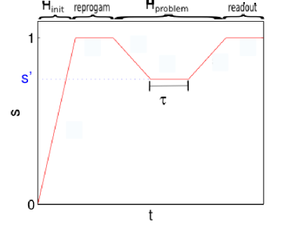
Figure 1: Schematic representation of a single annealing cycle to perform a local search. First the standard QAA is implemented with the problem Hamiltonian given in Eq. (1) to initialize the qubits in the desired state. After this the Hamiltonian is reprogrammed and the device is annealed to $s^{\prime}$ and optionally allowed to remain at that point for a time $\tau$. The device is then annealed to $s=1$ and read out.

References

- [1]
- [2] S. H. Adachi & M. P. Henderson (2015): Application of Quantum Annealing to Training of Deep Neural Networks. Available at https://arxiv.org/abs/1510.06356.
- [3] E. Farhi, J. Goldstone, S. Gutmann, J. Lapan, A. Lundgren & D. Preda (2001): A quantum adiabatic evolution algorithm applied to random instances of an NP-complete problem. Science 292, pp. 472–475, 10.1126/science.1057726.
- [4] J. Brooke, D. Bitko, T. F. Rosenbaum & G. Aeppli (1999): Quantum annealing of a disordered magnet. Science 284, pp. 779–781, 10.1126/science.284.5415.779.
- [5] M. H. Amin, E. Andriyash, J. Rolfe, B. Kulchytskyy & R. Melko, (2016): Quantum Boltzmann Machine. Available at https://arxiv.org/abs/1601.02036.
- [6] M. W. Johnson et al. (2011): Quantum annealing with manufactured spins. Nature 473, pp. 194–198, 10.1038/nature10012.
- [7] N. Chancellor, S. Szoke, W. Vinci, G. Aeppli & P. A. Warburton, (2016): Maximum-Entropy Inference with a Programmable Annealer. Scientific Reports 6(22318), 10.1038/srep22318.
- [8] N. G. Dickson et al. (2013): Thermally assisted quantum annealing of a 16-qubit problem. Nature Communications 4(1903), 10.1038/ncomms2920.
- [9] S. Boixo et al. (2016): Computational Role of Multiqubit Tunneling in a Quantum Annealer. Nature Communications 7(10327), 10.1038/ncomms10327.
- [10] W. Vinci, K. Markström, S. Boixo, A. Roy, F. M. Spedalieri, P. A. Warburton & S. Severini (2014): Hearing the Shape of the Ising Model with a Programmable Superconducting-Flux Annealer. Scientific Reports 4(5703), 10.1038/srep05703.
- [11] Y. Otsubo, J. I. Inoue, K. Nagata & M. Okada (2012): Effect of quantum fluctuation in error-correcting codes. Physical Review E 86(051138), 10.1103/PhysRevE.86.051138.
- [12] Y. Otsubo, J. I. Inoue, K. Nagata & M. Okada (2014): Code-division multiple-access multiuser demodulator by using quantum fluctuations. Physical Review E 90(012126), 10.1103/PhysRevE.90.012126.
- [13] T. Albash, S. Boixo, D. A. Lidar & P. Zanardi (2014): Quantum Adiabatic Markovian Master Equations. New Journal of Physics 14(123016), 10.1088/1367-2630/14/12/123016.
- [14] H. P. Breuer & F. Petruccione (2002): The Theory of Open Quantum Systems. Oxford University Press.
- [15] N. Chancellor (to appear) Modernizing Quantum Annealing using Local Searches.
- [16] N. Chancellor, J. Morley, V. Kendon & S. Bose (in preparation): Adiabatic and quantum walk search algorithms as quantum annealing extremes.
- [17] N. Chancellor, P. A. Warburton & G. Aeppli (2016): Experimental Freezing of mid-Evolution Fluctuations with a Programmable Annealer. Available at http://arxiv.org/abs/arXiv:1605.07549.
- [18] V. Choi (2010): Adiabatic Quantum Algorithms for the NP-Complete Maximum-Weight Independent Set, Exact Cover and 3SAT Problems. Available at http://arxiv.org/abs/1004.2226.
- [19] G. E. Coxson, C. R. Hill & J. C. Russo (2014): Adiabatic quantum computing for finding low-peak-sidelobe codes. High Performance Extreme Computing conference, IEEE 7, pp. 3910–3916, 10.1039/b509983h.
- [20] D. J. Earl & M. W. Deem (2005): Parallel Tempering: Theory, Applications, and New Perspectives. Physical Chemistry Chemical Physics 7, pp. 3910–3916, 10.1039/b509983h.
- [21] A. B. Finilla, M. A. Gomez, C. Sebenik & J. D. Doll (1994): Quantum annealing: A new method for minimizing multidimensional functions. Chemical Physics Letters 219, pp. 343–348, 10.1016/0009-2614(94)00117-0.
- [22] K. Hukushima & Y. Iba (2003): The Monte Carlo Method in the Physical Sciences: Celebrating the 50th Anniversary of the Metropolis Algorithm. 690, AIP.
- [23] S. P. Jordan, E. Farhi & P. W. Shor (2006): Error-correcting codes for adiabatic quantum computation. Physical Review A 74(052322), 10.1103/PhysRevA.74.052322.
- [24] M. Marzec (2014): Portfolio Optimization: Applications in Quantum Computing. Social Science Research Network Technical Report, 10.2139/ssrn.2278729.
- [25] J. Matcha (2010): Population Annealing with Weighted Averages: A Monte Carlo Method for Rough Free Energy Landscapes. Physical Review E 82(026704), 10.1103/PhysRevE.82.026704.
- [26] R. H. Swendsen & J. S. Wang (1986): Replica Monte Carlo Simulation of Spin-Glasses. Physical Review Letters 57(2607), 10.1103/PhysRevLett.57.2607.
- [27] W. Wang, J. Matcha & H. G. Katzgraber (2015): Population annealing: Theory and application in spin glasses. Physical Review E 92(063307), 10.1103/PhysRevE.92.063307.
- [28] W. K. Wootters & W. H. Zurek (1982): A single quantum cannot be cloned. Nature 299, pp. 802–803, 10.1038/299802a0.
- [29] Z. Zhu, A. H. Ochoa & H. G. Katzgraber (2015): Efficient Cluster Algorithm for Spin Glasses in Any Space Dimension. Physical Review Letters 115(077201), 10.1103/PhysRevLett.115.077201.