Statistical mechanics of thin spherical shells

Abstract

We explore how thermal fluctuations affect the mechanics of thin amorphous spherical shells. In flat membranes with a shear modulus, thermal fluctuations increase the bending rigidity and reduce the in-plane elastic moduli in a scale-dependent fashion. This is still true for spherical shells. However, the additional coupling between the shell curvature, the local in-plane stretching modes and the local out-of-plane undulations, leads to novel phenomena. In spherical shells thermal fluctuations produce a radius-dependent negative effective surface tension, equivalent to applying an inward external pressure. By adapting renormalization group calculations to allow for a spherical background curvature, we show that while small spherical shells are stable, sufficiently large shells are crushed by this thermally generated “pressure”. Such shells can be stabilized by an outward osmotic pressure, but the effective shell size grows non-linearly with increasing outward pressure, with the same universal power law exponent that characterizes the response of fluctuating flat membranes to a uniform tension.

I Introduction

Continuum elastic theories for plates Love (1888); Föppl (1907); von Kármán (1910) and shells Sanders (1963); Koiter (1966) have been under development for over a century, but they are still actively explored, because of the “extreme mechanics” generated by geometrical nonlinearities Krieger (2012); Stoop et al. (2015). Initially, these theories were applied to the mechanics of thin macroscopic structures, where the relevant elastic constants (a Young’s modulus and a bending rigidity) are related to the bulk material properties and the plate or shell thickness. However, these theories have also been successfully applied to describe mechanical properties of microscopic structures, such as viral capsids Lidmar et al. (2003); Ivanovska et al. (2004); Michel et al. (2006); Klug et al. (2006), bacterial cell walls Yao et al. (1999); Wang et al. (2010); Nelson (2012); Amir et al. (2014), membranes of red blood cells Waugh and Evans (1979); Evans (1983); Park et al. (2010), and hollow polymer and polyelectrolyte capsules Gao et al. (2001); Gordon et al. (2004); Lulevich et al. (2004); Elsner et al. (2006); Zoldesi et al. (2008). Note that in these more microscopic examples, the effective elastic constants are not related to bulk mechanical properties, but instead depend on details of microscopic molecular interactions.

At the microscopic scale, thermal fluctuations become important and their effects on flat two dimensional solid membranes have been studied extensively, starting in the late 1980’s. Unlike long one dimensional polymers, which perform self-avoiding random walks de Gennes (1979); Doi and Edwards (1986), arbitrarily large two dimensional membranes remain flat at low temperatures due to the strong thermal renormalizations triggered by flexural phonons, Nelson and Peliti (1987) which result in strongly scale-dependent enhanced bending rigidities and reduced in-plane elastic constants. Nelson et al. (2004); Katsnelson (2012). A related scaling law for the membrane structure function of a solution of spectrin skeletons of red blood cells was checked in an ensemble-averaged sense via elegant X-ray and light scattering experiments. Schmidt et al. (1993) However, recent advances in growing and isolating free-standing layers of crystalline materials such as graphene, boron nitride or transition metal dichalcogenides Novoselov et al. (2005) (not adsorbed onto a bulk substrate or stretched across a supporting structure) hold great promise for exploring how flexural modes affect the mechanical properties of individual sheet polymers that are atomically thin. Recent experiments with graphene have in fact observed a $\sim$$4000$-fold enhancement of the bending rigidity, Blees et al. (2015) and a reduced Young’s modulus Nicholl et al. (2015), although these results may also be influenced by quenched random disorder (e.g., ripples or grain boundaries), which can compete with thermal fluctuations to produce similar effects Radzihovsky and Nelson (1991); Košmrlj and Nelson (2013, 2014).

While thermal fluctuations of flat solid sheets are well understood, many microscopic membranes correspond to closed shells, and much less is known about their response to thermal fluctuations. The simplest possible shell is an amorphous spherical shell. This was studied by Paulose et al. Paulose et al. (2012), where perturbative corrections to elastic constants at low temperatures and external pressures were derived and tested with Monte Carlo simulations. Remarkably, these simulations found that at high temperatures thermalized spheres begin to collapse at less than half the classical buckling pressure (see Fig. 1). However, it was not possible to quantify this effect, because the perturbative corrections diverge with shell radius. Here, we go well beyond perturbation theory by employing renormalization group techniques, which enable us to study spherical shells over a wide range of sizes, temperatures and external pressures. We show that while spherical shells retain some features of flat solid sheets, there are remarkable new phenomena, such as a thermally generated negative tension, which spontaneously crushes large shells even in the absence of external pressure. We find that shells can be crushed by thermal fluctuations even in the presence of a stabilizing outward pressure!

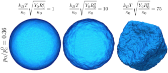
Figure 1: (Color online) Snapshots of thermalized spheres from Monte Carlo simulations under inward external pressure $p_{0}$ at $36\%$ of the classical buckling pressure $p_{c}^{0}$ at varying temperatures $T$. All three snapshots are for identical amorphous spherical shells with size $R_{0}=55a$ ($a$ is the average mesh size) with bending rigidity $\kappa_{0}=50\epsilon$ and Young’s modulus $Y_{0}=577\epsilon/a^{2}$ ($\epsilon$ sets the energy scale); the Föppl-von Karman number characterizing the nonlinear shell mechanics is $\gamma=Y_{0}R_{0}^{2}/\kappa_{0}\approx 35,000$. Shells are under the same inward external pressure $p_{0}=0.08\epsilon/a^{3}$, but they are at different temperatures $k_{B}T=0.267\epsilon$, $k_{B}T=2.67\epsilon$, $k_{B}T=20\epsilon$ (from left to right). Note that the shell on the right is crushed even though the inward external pressure pressure $p_{0}\approx 0.36p_{c}^{0}$ is much lower than the classical buckling pressure $p_{c}^{0}=4\sqrt{\kappa_{0}Y_{0}}/R_{0}^{2}$. Images are courtesy of Gerrit Vliegenthart and details of simulations are provided in Ref. Paulose et al. (2012).

In Sec. II, we review the shallow-shell theory description of thin elastic spheres, Sanders (1963); Koiter (1966) while in Sec. III we show how to set up the statistical mechanics leading to the thermal shrinkage and fluctuations in the local displacement normal to the shell. Low temperature, perturbative corrections to quantities such as the effective pressure $p$ (a sum of conventional and osmotic contributions), bending rigidity $\kappa$ and Young’s modulus $Y$ diverge like $\sqrt{\gamma}$, where $\gamma=Y_{0}R_{0}^{2}/\kappa_{0}$ is the Föppl-von Karman number of the shell with radius $R_{0}$ and microscopic elastic moduli $Y_{0}$ and $\kappa_{0}$. Paulose et al. (2012) A momentum shell renormalization group is then implemented directly for shells embedded in $d=3$ dimensions to resolve these difficulties in Sec. IV. At small scales the bending rigidity and Young’s modulus renormalize like flat sheets; however, at large scales the curvature of the shell produces significant changes. At low temperatures ($k_{B}T\sqrt{\gamma}/\kappa_{0}\ll 1$) the renormalization is cut off already at the elastic length $\ell_{\textrm{el}}=\left(\kappa_{0}R_{0}^{2}/Y_{0}\right)^{1/4}$. At large temperatures ($k_{B}T\sqrt{\gamma}/\kappa_{0}\gg 1$) and beyond an important thermal length scale $\ell_{\textrm{th}}\sim\kappa_{0}/\sqrt{k_{B}TY_{0}}$, the bending rigidity and Young’s modulus renormalize with length scale $\ell$ like flat sheets with $\kappa_{R}\approx\kappa_{0}(\ell/\ell_{\textrm{th}})^{\eta}$ and $Y_{R}\approx Y_{0}(\ell_{\textrm{th}}/\ell)^{\eta_{u}}$, where $\eta\approx 0.8$ and $\eta_{u}\approx 0.4$. Aronovitz and Lubensky (1988) However, this renormalization is interrupted as one scales out to the shell radius $R_{0}$. For zero pressure we find that shells become unstable to a finite wave-vector mode appearing at the scale $\ell^{*}\sim\ell_{\textrm{th}}[\ell_{\textrm{el}}/\ell_{\textrm{th}}]^{4/(2+\eta)}\propto R_{0}^{2/(2+\eta)}\ll R_{0}$. A sufficiently large (negative) outward pressure stabilizes the shell and leads to an alternative infrared cut off given by a pressure-dependent length scale $\ell_{p}$. Detailed results for correlation functions, renormalized couplings and the change in the shell radius can be obtained by integrating the renormalization group flow equations out to scales where the thermal averages are no longer singular. In Sec. IV, we also present a simple, intuitive derivation of the scaling relation $\eta_{u}+2\eta=2$, originally derived using Ward identities associated with rotational invariance in Ref. Aronovitz and Lubensky (1988); Guitter et al. (1989). In Sec. V, we use the renormalization group method to study the dependence of the renormalized buckling pressure $p_{c}$ on temperature, shell radius and the elastic parameters, which defines a limit of metastability for thermalized shells. The calculated scaling function $\Psi(x)$ defined by $p_{c}=p_{c}^{0}\Psi(k_{B}T\sqrt{\gamma}/\kappa_{0})$ gives a reasonable description of the buckling threshold found in simulations of thermalized shells Paulose et al. (2012) with no adjustable parameters. Especially interesting is a result that holds when the pressure difference $p$ between the inside and outside of the shell vanishes, as might be achievable experimentally by creating a hemispherical elastic shell, or a closed shell with regularly spaced large holes. In this case we find that thermal fluctuations must necessarily crush spherical shells larger than a certain temperature-dependent radius given by $R_{\textrm{max}}=c(\kappa_{0}/k_{B}T)\sqrt{\kappa_{0}/Y_{0}}$ where the numerical constant $c\approx 160$. Even shells with a small stabilizing outward pressure can be crushed by thermal fluctuations (see Fig. 5). We conclude in Sec. VI by estimating the importance of thermal fluctuations for a number of thin shells that arise naturally in biology and materials science. For a very thin polycrystalline monolayer shell of a graphene like material (so that it is approximately amorphous), this radius at room temperature is only $160\textrm{nm}$.

II Elastic energy of deformation

The elastic energy of a deformed thin spherical shell of radius $R_{0}$ can be estimated with a shallow-shell theory Sanders (1963); van der Heijden (2009), which considers a small patch of spherical shell that is nearly flat. This may seem a limiting description at first, but as discussed below, the shell response to thermal fluctuations is completely determined by a smaller elastic length scale

$$\ell_{\textrm{el}}=\left(\frac{\kappa_{0}R_{0}^{2}}{Y_{0}}\right)^{1/4}\sim\sqrt{R_{0}h}\ll R_{0},$$ (1)

where $\kappa_{0}$ is the microscopic bending rigidity, $Y_{0}$ is the microscopic Young’s modulus and we introduced the effective thickness $h\sim\sqrt{\kappa_{0}/Y_{0}}$. For thin shells we require that $h\ll R_{0}$ or equivalently that the Föppl-von Karman number $\gamma=Y_{0}R_{0}^{2}/\kappa_{0}\gg 1$. Lidmar et al. (2003)

For a nearly flat patch of spherical shell it is convenient to use the Monge representation near the South Pole to describe the reference undeformed surface

$${\bf X}_{u}(x,y)=x\hat{\bf e}_{x}+y\hat{\bf e}_{y}+w(x,y)\hat{\bf e}_{z},$$ (2)

where $w(x,y)\approx(x^{2}+y^{2})/(2R_{0})$, and then decompose the displacements of a thermally deformed shell configuration ${\bf X}_{d}(x,y)$ into tangential displacements $u_{i}(x,y)$ and radial displacements $f(x,y)$, such that

$${\bf X}_{d}={\bf X}_{u}+u_{x}\hat{\bf t}_{x}+u_{y}\hat{\bf t}_{y}+f\hat{\bf n},$$ (3)

where $\hat{\bf t}_{i}=[\hat{\bf e}_{i}+(\partial_{i}w)\hat{\bf e}_{z}]/\sqrt{1+(\partial_{i}w)^{2}}$ is a unit tangent vector, $\hat{\bf n}=[\hat{\bf e}_{z}-(\partial_{i}w)\hat{\bf e}_{i}]/\sqrt{1+\sum_{i}(\partial_{i}w)^{2}}$ is a unit normal vector that points inward from the South Pole and $i\in\{x,y\}$. Note that positive radial displacements $f(x,y)$ correspond to shrinking of the spherical shell. With this decomposition, the free energy cost of shell deformation can be described as van der Heijden (2009)

$$F=\int\!dxdy\ \left[\frac{\kappa_{0}}{2}(\nabla^{2}f)^{2}+\frac{\lambda_{0}}{2}u_{ii}^{2}+\mu_{0}u_{ij}^{2}-p_{0}f\right],$$ (4)

where summation over indices $i,j\in\{x,y\}$ is implied. The first term describes the bending energy with a microscopic bending rigidity $\kappa_{0}$ and next two terms describe the in-plane stretching energy with two-dimensional Lamé constants $\lambda_{0}$ and $\mu_{0}$; the corresponding Young’s modulus is $Y_{0}=4\mu_{0}(\mu_{0}+\lambda_{0})/(2\mu_{0}+\lambda_{0})$. The last term describes the external pressure work, where $p_{0}$ is a combination of hydrostatic and osmotic contributions. We assume that the interior and exterior of spherical shell is filled with a fluid such as water, which can pass freely through a semipermeable shell membrane on the relevant time scales. Additionally, there may be nonpermeable molecules inside or outside the shell giving rise (within ideal solution theory) to an osmotic pressure contribution $k_{B}T(c_{\textrm{out}}-c_{\textrm{in}})$. Phillips et al. (2013) Here, $c_{\textrm{out}}$ and $c_{\textrm{in}}$ are the concentrations of such molecules outside and inside the shell, respectively. Note that for $p_{0}>0$, introduction of thermal fluctuations into Eq. (4) requires that we deal with the statistical mechanics of a metastable state – a macroscopic inversion of the shell (“snap-through” transition) can lower the free energy, Landau and Lifshitz (1970) although often with a very large energy barrier.

In the shallow shell approximation the strain tensor is van der Heijden (2009)

$$u_{ij}=\frac{1}{2}(\partial_{i}u_{j}+\partial_{j}u_{i})+\frac{1}{2}(\partial_{i}f)(\partial_{j}f)-\delta_{ij}\frac{f}{R_{0}},$$ (5)

where $\delta_{ij}$ is the Kronecker delta. The first term describes the usual linear strains due to tangential displacements. The second describes similar in-plane strains due to displacements in the direction of the surface normals; this nonlinear term makes the analysis of thin plates and shells quite challenging. Nelson et al. (2004) The last term of Eq. (5), which linearly couples radial deformations $f(x,y)$ to the sphere curvature $1/R_{0}$, tells us that spherical shells cannot be bent without stretching, a striking change from flat plates where $R_{0}\rightarrow\infty$. The importance of this stretching can be estimated by considering a small radial deformation of amplitude $f_{0}$ over some characteristic length scale $\ell$, such that the non-linear term $(\partial_{i}f)(\partial_{j}f)/2$ in the strain tensor $u_{ij}$ is negligible. The bending energy cost scales as $\sim\kappa_{0}f_{0}^{2}/\ell^{4}$, while the stretching energy cost scales as $\sim Y_{0}f_{0}^{2}/R_{0}^{2}$. The bending energy dominates for deformations on small scales $\ell\ll\ell_{\textrm{el}}$, while the stretching energy cost dominates for deformations on large scales $\ell\gg\ell_{\textrm{el}}$, where the transition elastic length scale $\ell_{\textrm{el}}$ was defined in Eq. (1).

III Thermal fluctuations

The effects of thermal fluctuations are reflected in correlation functions obtained from functional integrals such as Nelson et al. (2004); Katsnelson (2012); Paulose et al. (2012)

$$\left<f_{0}\right>\equiv\left<f({\bf r}_{1})\right> = \frac{1}{Z}\int\!\mathcal{D}[u_{i},f]\ f({\bf r}_{1})e^{-F/k_{B}T},$$ (6a)

$$G_{ff}({\bf r_{2}}-{\bf r_{1}}) \equiv \left<\delta f({\bf r}_{1})\delta f({\bf r}_{2})\right>,$$

$$G_{ff}({\bf r_{2}}-{\bf r_{1}}) = \frac{1}{Z}\int\!\mathcal{D}[u_{i},f]\ \delta f({\bf r}_{1})\delta f({\bf r}_{2})e^{-F/k_{B}T},$$

$$Z = \int\!\mathcal{D}[u_{i},f]e^{-F/k_{B}T},$$ (6c)

where $T$ is the ambient temperature, $k_{B}$ is Boltzmann’s constant, ${\bf r}\equiv(x,y)$ and $\delta f({\bf r})=f({\bf r})-\left<f_{0}\right>$. Here, $f_{0}$ represents the uniform part of the fluctuating contraction or dilation of the spherical shell. One can define similar correlation functions for tangential displacements $u_{i}(x,y)$, but they are not the main focus of this study.

Besides separating tangential displacements $u_{i}({\bf r})$ and radial displacements $f({\bf r})$, it is also useful to further decompose radial displacements as $f({\bf r})=f_{0}+\tilde{f}({\bf r})$, where $f_{0}$ is the uniform part of the fluctuating radial displacement defined in the above paragraph. The quantity $\tilde{f}({\bf r})$ is then the deformation with respect to $f_{0}$, such that $\frac{1}{A}\int\!d^{2}{\bf r}\,\tilde{f}=\langle\tilde{f}\rangle=0$, where $A$ is the area. Finally, it is convenient to integrate out the in-plane phonon degrees of freedom $u_{i}({\bf r})$ as well as $f_{0}$ and study the effective free energy for radial displacements. The effective free energy then becomes Paulose et al. (2012)

$$F_{\textrm{eff}} = -k_{B}T\ln\left(\int\mathcal{D}[u_{i},f_{0}]e^{-F/k_{B}T}\right),$$ (7a)

$$F_{\textrm{eff}} = \int\!d^{2}{\bf r}\left(\frac{1}{2}\left[\kappa_{0}(\nabla^{2}\tilde{f})^{2}-\frac{p_{0}R_{0}}{2}|\nabla\tilde{f}|^{2}+\frac{Y_{0}\tilde{f}^{2}}{R_{0}^{2}}\right]\right.$$

$$\left.+\frac{Y_{0}}{8}\left[P_{ij}^{T}(\partial_{i}\tilde{f})(\partial_{j}\tilde{f})\right]^{2}-\frac{Y_{0}\tilde{f}}{2R_{0}}\left[P_{ij}^{T}(\partial_{i}\tilde{f})(\partial_{j}\tilde{f})\right]\right),$$

where $P_{ij}^{T}=\delta_{ij}-\partial_{i}\partial_{j}/\nabla^{2}$ is the transverse projection operator. From the effective free energy above, we see that an inward pressure $p_{0}$ acts like a negative surface tension $\sigma=-p_{0}R_{0}/2$. (A negative outward pressure $p_{0}<0$ would stabilize the shell, similar to a conventional surface tension.) The two terms that involve both the Young’s modulus $Y_{0}$ and radius $R_{0}$ are new for spherical shells, and arise from the coupling between radial displacements and in-plane stretching induced by the Gaussian curvature [see Eq. (5)]. Note that the last term of Eq. (LABEL:eq:effective_free_energy) breaks the symmetry between inward and outward normal displacements $\tilde{f}(x,y)$ of the shell.

Functional integrals similar to those in Eqs. (6) and Eq. (7a) determine the average contraction of a spherical shell

$$\left<f_{0}\right>=\left<f({\bf r}_{1})\right>=\frac{p_{0}R_{0}^{2}}{4(\mu_{0}+\lambda_{0})}+\frac{R_{0}}{4}\left<|\nabla\tilde{f}|^{2}\right>,$$ (8)

where the first term, controlled by the bulk modulus $\mu_{0}+\lambda_{0}$, describes the usual mechanical shrinkage due to an inward external pressure $p_{0}>0$, and the second describes additional contraction due to thermal fluctuations. This additional shrinking arises because nonuniform radial fluctuations $\tilde{f}({\bf r})$ at fixed radius would increase the integrated area, with a large stretching energy cost. The system prefers to wrinkle and shrink its radius to gain entropy, while keeping the integrated area of the convoluted shell approximately constant.

The effective free energy for radial displacements $\tilde{f}({\bf r})$ in Eq. (LABEL:eq:effective_free_energy) suggests that the Fourier transform of the correlation function $G_{ff}({\bf q})=\int\!(d^{2}{\bf r}/A)e^{-i{\bf q}\cdot{\bf r}}G_{ff}({\bf r})$ can be represented as Paulose et al. (2012)

$$G_{ff}({\bf q}) = \left<|\tilde{f}({\bf q})|^{2}\right>$$

$$G_{ff}({\bf q}) = \frac{k_{B}T}{A\left[\kappa_{R}(q)q^{4}-\frac{1}{2}p_{R}(q)R_{0}q^{2}+\frac{Y_{R}(q)}{R_{0}^{2}}\right]},$$ (9)

where $A$ is the area of a patch of spherical shell. The functional form in Eq. (9) above is dictated by quadratic terms in Eq. (LABEL:eq:effective_free_energy); the effect of the anharmonic terms is to replace bare parameters $\kappa_{0}$, $Y_{0}$ and $p_{0}$ with the scale dependent renormalized parameters $\kappa_{R}(q)$, $Y_{R}(q)$ and $p_{R}(q)$ as was shown previously for solid flat membranes in the presence of thermal fluctuations Nelson et al. (2004); Katsnelson (2012). Note that the last term in the denominator of Eq. (9) suppresses radial fluctuations due to the stretching energy cost and makes them finite even for long wavelength modes (small $q$). Conversely, the amplitude of long wavelength fluctuations diverges more strongly in the limit $R_{0}\rightarrow\infty$ of large shells.

Before we discuss the renormalizing effect of nonlinearities in Eq. (LABEL:eq:effective_free_energy), it is useful to note that for large inward external pressure $p_{0}>0$, the denominator in Eq. (9) can become negative for certain wavevectors ${\bf q}$, which indicates that these radial deformation modes $\tilde{f}({\bf q})$ become unstable. Paulose et al. (2012) If we neglect nonlinear effects, and replace the renormalized couplings $\kappa_{R}$, $Y_{R}$ and $p_{R}$ by their bare values, the minimal value of external pressure $p_{c}^{0}$, where these modes first become unstable, is

$$p_{c}^{0}=\frac{4\sqrt{\kappa_{0}Y_{0}}}{R_{0}^{2}},$$ (10)

which corresponds to the classical buckling pressure for spherical shells van der Heijden (2009). The magnitude of the wavevectors ${\bf q}_{c}$ for the unstable modes at the critical external pressure $p_{c}^{0}$ is Hutchinson (1967)

$$q_{c}=\left(\frac{Y_{0}}{\kappa_{0}R_{0}^{2}}\right)^{1/4}=\ell_{\textrm{el}}^{-1}.$$ (11)

When these ideas are extended to finite temperatures, this threshold becomes a limit of metastability, and we expect hysteresis loops as the external pressure is cycled up and down. Katifori et al. (2010)

Some insights into the statistical mechanics associated with Eqs. (7a) and (LABEL:eq:effective_free_energy) follows from calculating the renormalized bending rigidity, Young’s modulus and effective pressure at long wavelengths via low temperature perturbation theory in $k_{B}T/\kappa_{0}$. When the external pressure is zero, Paulose et al. found that Paulose et al. (2012)

$$\kappa_{R} \approx \kappa_{0}\left[1+\frac{61}{4096}\frac{k_{B}T}{\kappa_{0}}\sqrt{\gamma}\right],$$ (12a)

$$Y_{R} \approx Y_{0}\left[1-\frac{3}{256}\frac{k_{B}T}{\kappa_{0}}\sqrt{\gamma}\right],$$ (12b)

$$p_{R} \approx \frac{p_{c}^{0}}{24\pi}\frac{k_{B}T}{\kappa_{0}}\sqrt{\gamma},$$ (12c)

where $\gamma=Y_{0}R_{0}^{2}/\kappa_{0}$ is the Föppl-von Karman number and the critical pressure parameter $p_{c}^{0}$ is given by Eq. (10). Perturbation theory reveals that thermal fluctuations enhance the bending rigidity and soften the Young’s modulus. However, the corrections to $\kappa_{R}$ and $Y_{R}$ are multiplied by $\sqrt{\gamma}$, which diverges as the radius $R_{0}$ of the thermalized sphere tends to infinity. Especially striking is a similar divergence in the effective pressure $p_{R}$, see Eq. (12c). Evidently, even if the microscopic pressure difference $p_{0}$ between the inside and outside of sphere is zero, thermal fluctuations will nevertheless generate an effective pressure that eventually exceeds the buckling instability of the sphere for sufficiently large $R_{0}$. A naive estimate for the critical radius $R_{\textrm{max}}$ can be obtained by requiring that the renormalized pressure $p_{R}$ becomes equal to the buckling pressure $p_{c}^{0}$ in Eq. (12c), which leads to $R_{\textrm{max}}\approx c[\kappa_{0}/k_{B}T]\sqrt{\kappa_{0}/Y_{0}}$ with $c=24\pi\approx 75$. Some evidence in this direction already appears in the computer simulations of Ref. Paulose et al. (2012), where amorphous thermalized spheres already begin to collapse at less than half the classical buckling pressure (see also Fig. 1, where the pressure is $36\%$ of $p_{c}^{0}$). Similar perturbative divergences in the bending rigidity and Young’s modulus of flat membranes of size $R_{0}$ (here the corrections diverge with $\gamma$ rather than $\sqrt{\gamma}$ Nelson et al. (2004)) can be handled with integral equation methods, Nelson and Peliti (1987); Le Doussal and Radzihovsky (1992) which sum contributions to all orders in perturbation theory, or alternatively, with the renormalization group. Aronovitz and Lubensky (1988) It is this latter approach we take in the next Section.

IV Perturbative renormalization group

The effect of the anharmonic terms in Eq. (LABEL:eq:effective_free_energy) at a given scale $\ell^{*}\equiv\pi/q^{*}$ can be obtained by systematically integrating out all degrees of freedom on smaller scales (i.e., larger wavevectors). Formally this renormalization group transformation proceeds by splitting radial displacements $\tilde{f}({\bf r})$ into slow modes $\tilde{f}_{<}({\bf r})=\sum_{|\bf{q}|<q^{*}}e^{i{\bf q}\cdot{\bf r}}\tilde{f}({\bf q})$ and fast modes $\tilde{f}_{>}({\bf r})=\sum_{|\bf{q}|>q^{*}}e^{i{\bf q}\cdot{\bf r}}\tilde{f}({\bf q})$, which are then integrated out as

$$F_{\textrm{eff}}(\ell^{*})=-k_{B}T\ln\left(\int\!\mathcal{D}[\tilde{f}_{>}]\ e^{-F_{\textrm{eff}}/k_{B}T}\right).$$ (13)

These functional integrals can be approximately evaluated with standard perturbative renormalization group calculations Amit and Mayor (2005) and lead to an effective free energy with the same form as in Eq. (LABEL:eq:effective_free_energy), except that renormalized parameters become scale dependent, i.e. they are replaced by $\kappa_{R}(\ell^{*})$, $Y_{R}(\ell^{*})$ and $p_{R}(\ell^{*})$.

To implement this momentum shell renormalization group, we first integrate out all Fourier modes in a thin momentum shell $\Lambda/b<q<\Lambda$, where $a=\pi/\Lambda$ is a microscopic cutoff (e.g. the shell thickness) and $b\equiv\ell/a=e^{s}$ with $s\ll 1$. Next we rescale lengths and fields Aronovitz and Lubensky (1988); Radzihovsky and Nelson (1991)

$${\bf r} = b{\bf r}^{\prime},$$ (14a)

$$\tilde{f}({\bf r}) = b^{\zeta_{f}}\tilde{f}^{\prime}({\bf r}^{\prime}),$$ (14b)

where the field rescaling exponent $\zeta_{f}$ will be chosen to simplify the resulting renormalization group equations. We find it convenient to work directly with a $D=2$ dimensional spherical shell embedded in $d=3$ space, rather than introducing an expansion in $\epsilon=4-D$. Aronovitz and Lubensky (1988) Finally, we define new elastic constants $\kappa^{\prime}$, $Y^{\prime}$, and a new external pressure $p^{\prime}$, such that the free energy functional in Eq. (LABEL:eq:effective_free_energy) retains the same form after the first two renormalization group steps. It is common to introduce $\beta$ functions Amit and Mayor (2005), which define the renormalization flow of elastic constants. It is not possible to calculate these $\beta$ functions exactly, but one can use diagrammatic techniques Amit and Mayor (2005) to obtain systematic approximations in the limit $s\ll 1$. To one loop order (see Fig. 2) the renormalization group flows are given by

$$\beta_{\kappa} = \frac{d\kappa^{\prime}}{ds}=2(\zeta_{f}-1)\kappa^{\prime}+\frac{3k_{B}TY^{\prime}\Lambda^{2}}{16\pi\mathcal{D}}$$ (15a)

$$\quad\quad\quad-\frac{3k_{B}TY^{\prime 2}\Lambda^{2}}{8\pi R^{\prime 2}\mathcal{D}^{2}}\bigg{[}1+\frac{I_{\kappa 1}}{\mathcal{D}^{2}}+\frac{I_{\kappa 2}}{\mathcal{D}^{4}}\bigg{]},$$

$$\beta_{Y} = \frac{dY^{\prime}}{ds}=2\zeta_{f}Y^{\prime}-\frac{3k_{B}TY^{\prime 2}\Lambda^{6}}{32\pi\mathcal{D}^{2}},$$ (15b)

$$\beta_{p} = \frac{dp^{\prime}}{ds}=(2\zeta_{f}+1)p^{\prime}+\frac{3k_{B}TY^{\prime 2}\Lambda^{4}}{4\pi R^{\prime 3}\mathcal{D}^{2}}\left[1+\frac{I_{p}}{\mathcal{D}^{2}}\right],\quad\$$ (15c)

$$\beta_{R} = \frac{dR^{\prime}}{ds}=-R^{\prime},$$ (15d)

where we introduced the denominator term

$$\mathcal{D} = \kappa^{\prime}\Lambda^{4}-\frac{p^{\prime}R^{\prime}\Lambda^{2}}{2}+\frac{Y^{\prime}}{R^{\prime 2}}.$$ (16)

The derivation of recursion relations in Eq. (15) is given in the Appendix A, where we also provide detailed expressions for $I_{\kappa 1}$, $I_{\kappa 2}$ and $I_{p}$ in Eq. (52).

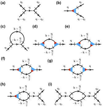
Figure 2: (Color online) Feynman diagrams contributing to the renormalization flows of Eq. (15). (a) Four-point and (b) three-point vertices describe the quartic and cubic terms in the free energy Eq. (LABEL:eq:effective_free_energy). Legs represent radial displacement fields $\tilde{f}({\bf q})$ and slashes on legs correspond to spatial derivatives, which lead to additional factors of wave vectors in the Fourier space. The red part of the three-point vertex in (b) connects to a field without a slash, while the blue parts connect to derivative terms. The four-point vertex carries a factor $Y$, while the three-point vertex carries a factor $Y/R$ (c-i) One-loop diagrams that contribute to the renormalization flows of (c-g) the bending rigidity $\kappa_{R}$, (f-g) the external pressure $p_{R}$, and (g) the Young’s modulus $Y_{R}$ in the propagator $G_{ff}({\bf q})$ in Eq. (9). Diagrams (h) and (i) describe one-loop contributions to the renormalization flows of the Young’s modulus $Y_{R}$ associated with three-point and four-point vertices, respectively. The connected legs in these diagrams represent the propagators $G_{ff}({\bf q})$, with wave vectors ${\bf k}$ restricted to the momentum shell $\Lambda/b<k<\Lambda$.

The $\beta_{Y}$ recursion relation in Eq. (15b) describes changes in the quadratic “mass” proportional to $Y$ in Eq. (LABEL:eq:effective_free_energy). Similarly, we can calculate the recursion relations for the cubic and quartic terms in Eq. (LABEL:eq:effective_free_energy) and we find that the only significant change is that the $2\zeta_{f}Y$ term now becomes $(3\zeta_{f}-1)Y$ and $(4\zeta_{f}-2)Y$, respectively. To ensure that the free energy retains the same form after the first two steps in the renormalization procedure, we choose $\zeta_{f}=1$, so that these three terms renormalize in tandem. The final results are independent of the precise choice of $\zeta_{f}$, as illustrated in Appendix B for thermalized flat sheets.

The scale-dependent parameters $\kappa^{\prime}(s)$, $Y^{\prime}(s)$, and $p^{\prime}(s)$, obtained by integrating the differential equations in Eqs. (15) up to a scale $s=\ln(\ell/a)$ with initial conditions $\kappa^{\prime}(0)=\kappa_{0}$, $Y^{\prime}(0)=Y_{0}$ and $p^{\prime}(0)=p_{0}$, are related to the scaling of propagator $G_{ff}(q)$ as Amit and Mayor (2005)

$$\!\!G_{ff}(q|\kappa_{0},p_{0},Y_{0},R_{0},A)=\left<|f({\bf q})|^{2}\right>=e^{2\zeta_{f}s}\left<|f^{\prime}({\bf q}^{\prime})|^{2}\right>$$

$$\!\!=e^{2\zeta_{f}s}G_{ff}(qe^{s}|\kappa^{\prime}(s),p^{\prime}(s),Y^{\prime}(s),R_{0}e^{-s},Ae^{-2s}),$$ (17)

where we explicitly insert the rescaled momenta $q^{\prime}=qe^{s}$, the rescaled radius $R^{\prime}=R_{0}e^{-s}$ and the rescaled patch area $A^{\prime}=Ae^{-2s}$. By replacing the left hand side in the Eq. (17) above with the renormalized propagator $G_{ff}(q)$ in Eq.(9), we find the scale-dependent renormalized parameters

$$\kappa_{R}(s) = \kappa^{\prime}(s)e^{(2-2\zeta_{f})s}=\kappa^{\prime}(s),$$ (18a)

$$Y_{R}(s) = Y^{\prime}(s)e^{(-2\zeta_{f})s}=Y^{\prime}(s)e^{-2s},$$ (18b)

$$p_{R}(s) = p^{\prime}(s)e^{(-1-2\zeta_{f})s}=p^{\prime}(s)e^{-3s},$$ (18c)

where we used $\zeta_{f}=1$ and parameter $s$ is related to the length scale $\ell=ae^{s}$ or equivalently to the magnitude of wavevector $q\equiv\pi/\ell$.

Note that by sending the shell radius to infinity ($R_{0}\rightarrow\infty$) and the pressure $p_{0}\rightarrow 0$, such that the product $\sigma=-p_{0}R_{0}/2$ remains fixed in Eq. (LABEL:eq:effective_free_energy), we recover the renormalization flows for solid flat membranes with the addition of a tension $\sigma$. Radzihovsky and Nelson (1991); Košmrlj and Nelson (2016) However, for spherical shells with finite $R_{0}$ thermal fluctuations renormalize and effectively increase the external pressure [see Eq. (15c)], in striking contrast to the behavior of flat membranes. Note, in particular, that an effective pressure is generated by Eq. (15c), even if the microscopic pressure $p_{0}$ vanishes!

Before discussing the detailed renormalization group predictions for spherical shells, it is useful to recall that for flat membranes with no tension, thermal fluctuations become important on scales larger than thermal length Nelson and Peliti (1987); Aronovitz and Lubensky (1988); Radzihovsky and Nelson (1991); Košmrlj and Nelson (2016); Guitter et al. (1989)

$$\ell_{\textrm{th}}=\sqrt{\frac{16\pi^{3}\kappa_{0}^{2}}{3k_{B}TY_{0}}},$$ (19)

and the renormalized elastic constants become strongly scale-dependent,

$$\kappa_{R}(\ell) \sim \left\{\begin{array}[]{c l}\kappa_{0},&\ell\ll\ell_{\textrm{th}}\\ \kappa_{0}(\ell/\ell_{\textrm{th}})^{\eta},&\ell_{\textrm{th}}\ll\ell\end{array}\right.,$$ (22)

$$Y_{R}(\ell) \sim \left\{\begin{array}[]{c l}Y_{0},&\ell\ll\ell_{\textrm{th}}\\ Y_{0}(\ell/\ell_{\textrm{th}})^{-\eta_{u}},&\ell_{\textrm{th}}\ll\ell\\ \end{array}\right.,$$ (25)

where $\eta\approx 0.80$-$0.85$ Nelson and Peliti (1987); Aronovitz and Lubensky (1988); Radzihovsky and Nelson (1991); Guitter et al. (1989); Le Doussal and Radzihovsky (1992); Košmrlj and Nelson (2016) and the exponents $\eta$ and $\eta_{u}$ are connected via a Ward identity $\eta_{u}+2\eta=2$ associated with rotational invariance. Aronovitz and Lubensky (1988); Guitter et al. (1989) In the one-loop approximation used here for 2d membranes embedded in three dimensions we obtain Košmrlj and Nelson (2016) $\eta=0.80$, which is adequate for our purposes. In the absence of an external tension, the renormalized bending rigidity $\kappa_{R}$ can become very large and the renormalized Young’s modulus $Y_{R}$ can become very small for large solid membranes in the flat phase, as seems to be the case for graphene. Blees et al. (2015); Nicholl et al. (2015) However, positive external tension acts as an infrared cutoff and the renormalized constants remain finite beyond a tension-induced length scale. Košmrlj and Nelson (2016); Roldan et al. (2011)

Although the scaling relation $\eta_{u}+2\eta=2$ originally arose from a Ward identity, Aronovitz and Lubensky (1988); Guitter et al. (1989) an alternative derivation provides additional physical insight: Suppose we are given a two-dimensional material (graphene, MoS₂, the spectrin skeleton of red blood cells, etc.) with a 2d Young’s modulus $Y_{0}$ and a 2d bending rigidity $\kappa_{0}$. With these material parameters we associate the elastic constants of an equivalent isotropic bulk material with 3d Young’s modulus $E_{0}$, 3d Poisson’s ratio $\nu_{0}$ and thickness $h$ by Landau and Lifshitz (1970)

$$\kappa_{0}=\frac{E_{0}h^{3}}{12(1-\nu_{0}^{2})},\quad Y_{0}=E_{0}h.$$ (26)

When thermal fluctuations are considered, we obtain the scale-dependent, 2d elastic parameters displayed in Eq. (25), $\kappa_{R}(\ell)\approx\kappa_{0}(\ell/\ell_{\textrm{th}})^{\eta}$ and $Y_{R}(\ell)\approx Y_{0}(\ell/\ell_{\textrm{th}})^{-\eta_{u}}$, where $\ell_{\textrm{th}}\ll\ell\ll L$, $L$ is the system size and the corresponding scale-dependent 2d Poisson’s ratio $\nu(\ell)$ remains of order unity. Aronovitz and Lubensky (1988) From these results and equation (26) we can define a scale-dependent effective thickness $h^{2}_{\textrm{eff}}(\ell)\sim\kappa_{R}(\ell)/Y_{R}(\ell)$, so that

$$h^{2}_{\textrm{eff}}(\ell)\sim h^{2}\left(\ell/\ell_{\textrm{th}}\right)^{\eta+\eta_{u}}.$$ (27)

For a $10\mu\textrm{m}\times 10\mu\textrm{m}$ square graphene, where $\ell_{\textrm{th}}\approx 1nm$ at room temperature, this thermal amplification (assuming $\eta+\eta_{u}\approx 0.8+0.4=1.2$) converts an atomic thickness to an effective thickness, whose ratio to the size of graphene sheet matches that of the ordinary writing paper, suggesting that room temperature graphene ribbons and springs can be studied with simple paper models. Blees et al. (2015) To determine a scaling relation between $\eta$ and $\eta_{u}$, we note that an alternative definition of the effective thickness follows from Nelson et al. (2004)

$$h^{2}_{\textrm{eff}}(\ell) = \left<f({\bf r})^{2})\right>_{\ell}$$

$$h^{2}_{\textrm{eff}}(\ell) = \int_{|\bf q|\geq\pi/\ell}\frac{d^{2}{\bf q}}{(2\pi)^{2}}\frac{k_{B}T}{\kappa_{R}(q)q^{4}}\sim\ell^{2-\eta},$$ (28)

where the average is evaluated over a $\ell\times\ell$ patch of the membrane, so that $q\geq\pi/\ell$ in the integration. Requiring similar scaling of Eqs. (27) and (28) with $\ell$ leads to $\eta_{u}+2\eta=2$.

By rewriting the renormalization group flows in Eq. (15) in dimensionless form it is easy to see that the renormalized parameters can be expressed in terms of the following scaling functions of dimensionless important length scales and of $p_{0}/p_{c}^{0}$, where $p_{c}^{0}$ is the classical buckling pressure in Eq. (10).

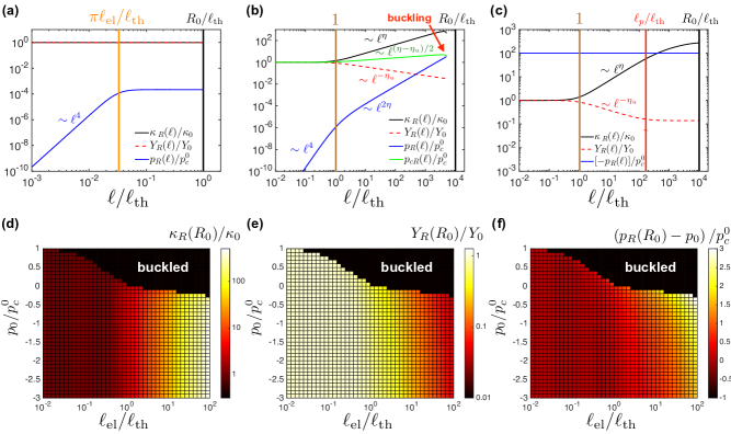
Figure 3: (Color online) Typical renormalization group flows at various microscopic pressures $p_{0}$ and ratios of $\ell_{\textrm{el}}=(\kappa_{0}R_{0}^{2}/Y_{0})^{1/4}$ to $\ell_{\textrm{th}}=\sqrt{16\pi^{3}\kappa_{0}/(3k_{B}TY_{0})}$. (a) Spherical shells at low temperature with $\ell_{\textrm{el}}/\ell_{\textrm{th}}=10^{-2}$, $R_{0}/\ell_{\textrm{th}}=1$, $a/R_{0}=10^{-6}$ and zero external pressure ($p_{0}=0$). In this case, there is practically no renormalization of the elastic constants $\kappa_{R}$ and $Y_{R}$, while the renormalization of the thermally generated external pressure $p_{R}$ is cut off at $\ell\approx\pi\ell_{\textrm{el}}$. (b-c) Spherical shells at high temperature with $\ell_{\textrm{el}}/\ell_{\textrm{th}}=10^{2}$, $R_{0}/\ell_{\textrm{th}}=10^{4}$, $a/R_{0}=10^{-6}$, and (b) zero external pressure ($p_{0}=0$) or (c) large stabilizing outward pressure ($p_{0}/p_{c}=-100$). In both these cases the elastic constants $\kappa_{R}$ and $Y_{R}$ initially renormalize in the same way as flat membranes [see Eq. (25)]. In case (b), even in the absence of external pressure $p_{0}=0$, this large shell buckles, because the thermally generated inward pressure $p_{R}(\ell)$ eventually reaches the renormalized critical buckling pressure $p_{cR}(\ell)$. In case (c) with a large outward pressure ($p_{0}<0$), spherical shells remain stable and the renormalization of elastic constants is cut off at the scale $\ell_{p}/\ell_{\textrm{th}}\sim(p_{c}^{0}/|p_{0}|)^{1/(2-\eta)}(\ell_{\textrm{el}}/\ell_{\textrm{th}})^{2/(2-\eta)}\sim\left(k_{B}TY_{0}/|p_{0}|R_{0}\kappa_{0}\right)^{1/(2-\eta)}$, which is analogous to the cut off prowided by an outward in-plane tension in flat solid membranes Košmrlj and Nelson (2016). For sufficiently large internal pressure $p_{0}\lesssim-k_{B}TY_{0}/R_{0}\kappa_{0}$ (not shown) the renormalization of $\kappa$ and $Y$ is completely suppressed. (d-f) Heat maps of (d) the renormalized bending rigidity $\kappa_{R}(R_{0})$, (e) the renormalized Young’s modulus $Y_{R}(R_{0})$, and (f) the thermally induced part of renormalized external pressure $p_{R}(R_{0})-p_{0}$ evaluated at the scale of the shell radius $R_{0}$. In (d-f) we used $R_{0}/\ell_{\textrm{el}}=10^{2}$ and $a/R_{0}=10^{-6}$. The large black buckled region is a direct consequence of thermal fluctuations. Note that both positive (inward) and negative (outward) pressures appear along the y-axis.

$$\kappa_{R}(\ell) = \kappa_{0}\,\Phi_{\kappa}\left(\frac{\ell}{\ell_{\textrm{th}}},\frac{\ell_{\textrm{el}}}{\ell_{\textrm{th}}},\frac{p_{0}}{p_{c}^{0}},\frac{a}{\ell_{\textrm{th}}}\right),$$ (29a)

$$Y_{R}(\ell) = Y_{0}\,\Phi_{Y}\left(\frac{\ell}{\ell_{\textrm{th}}},\frac{\ell_{\textrm{el}}}{\ell_{\textrm{th}}},\frac{p_{0}}{p_{c}^{0}},\frac{a}{\ell_{\textrm{th}}}\right),$$ (29b)

$$p_{R}(\ell) = p_{c}^{0}\,\Phi_{p}\left(\frac{\ell}{\ell_{\textrm{th}}},\frac{\ell_{\textrm{el}}}{\ell_{\textrm{th}}},\frac{p_{0}}{p_{c}^{0}},\frac{a}{\ell_{\textrm{th}}}\right).$$ (29c)

We expect that the scaling functions above are insensitive to the choice of microscopic cutoff $a$ (e.g. shell thickness or a carbon-carbon spacing in a large spherical buckyball), provided this cutoff is much smaller than other relevant lengths ($a\ll\ell_{\textrm{th}},\ell_{\textrm{el}}$). In principle, we could evaluate renormalized parameters on the whole interval $\ell\in[a,R]$, but for some values of bare parameters $\kappa_{0}$, $Y_{0}$, $p_{0}$ the renormalization flows in Eq. (15) diverge, when denominators become zero. This singularity indicates the buckling of thermalized spherical shells, which occurs when the renormalized external pressure $p_{R}(\ell^{*})$ reaches the renormalized critical buckling pressure

$$p_{cR}(\ell^{*})\equiv\frac{4\sqrt{\kappa_{R}(\ell^{*})Y_{R}(\ell^{*})}}{R_{0}^{2}},$$ (30)

where $\ell^{*}$ corresponds to the length scale of the unstable mode. In order for the shell to remain stable in the presence of thermal fluctuations, the renormalized pressure $p_{R}(\ell)$ has to remain below the renormalized critical buckling pressure $p_{cR}(\ell)$ for every $\ell\in[a,R_{0}]$.

Fig. 3 displays some typical flows of renormalized parameters. We find that for spherical shells the renormalized elastic constants, initially renormalize in the same way as for flat membranes [see Eq. (25)], but these singularities are eventually cut off by the Gaussian curvature. At low temperatures ($\ell_{\textrm{el}}/\ell_{\textrm{th}}\propto\sqrt{k_{B}T/\kappa_{0}}\gamma^{1/4}\ll 1$) and small inward pressures $p_{0}$, the corrections to renormalized bending rigidity $\kappa_{R}(\ell)/\kappa_{0}$ and renormalized Young’s modulus $Y_{R}(\ell)/Y_{0}$ grow as $(k_{B}T/\kappa_{0})Y_{0}\ell^{2}/\kappa_{0}$, while the renormalized pressure $p_{R}(\ell)-p_{0}$ grows as $k_{B}TY_{0}^{2}\ell^{4}/(\kappa_{0}^{2}R_{0}^{3})$. The renormalization is cut off at the elastic length scale $\ell_{\textrm{el}}$ (see Fig. 3a), where the $Y^{\prime}/R^{\prime 2}$ term starts dominating over the $\kappa^{\prime}\Lambda^{4}$ term in denominators $\mathcal{D}$ of the recursion relations in Eqs. (15). This cutoff gives rise to corrections of size $(k_{B}T/\kappa_{0})\sqrt{Y_{0}R_{0}^{2}/\kappa_{0}}$ [see Eq. (12)] for spherical shells, in contrast to the corrections of size $(k_{B}T/\kappa_{0})Y_{0}L_{0}^{2}/\kappa_{0}$ for flat sheets of size $L_{0}$.

At high temperatures ($\ell_{\textrm{el}}/\ell_{\textrm{th}}\propto\sqrt{k_{B}T/\kappa_{0}}\gamma^{1/4}\gg 1$) and small external pressures $p_{0}$, the corrections to the renormalized parameters $\kappa_{R}(\ell)$, $Y_{R}(\ell)$, $p_{R}(\ell)$ initially still grow in the same way as described above for low temperatures. However, a transition to the new regime happens at the thermal length scale $\ell_{\textrm{th}}\sim\kappa_{0}/\sqrt{k_{B}TY_{0}}$, where corrections to the renormalized bending rigidity $\kappa_{R}(\ell_{\textrm{th}})/\kappa_{0}$ and the renormalized Young’s modulus $Y_{R}(\ell_{\textrm{th}})/Y_{0}$ become of order unity and the renormalized pressure is $p_{R}(\ell_{\textrm{th}})-p_{0}\sim p_{c}^{0}(\ell_{\textrm{th}}/\ell_{\textrm{el}})^{2}\ll p_{c}^{0}$. On scales larger than the thermal length scale the renormalized parameters scale according to

$$\kappa_{R}(\ell) \sim \kappa_{0}(\ell/\ell_{\textrm{th}})^{\eta},$$ (31a)

$$Y_{R}(\ell) \sim Y_{0}(\ell/\ell_{\textrm{th}})^{-\eta_{u}},$$ (31b)

$$p_{R}(\ell)-p_{0} \sim p_{c}^{0}(\ell_{\textrm{th}}/\ell_{\textrm{el}})^{2}(\ell/\ell_{\textrm{th}})^{2\eta},$$ (31c)

where $\eta=0.8$ and $\eta_{u}=0.4$ are the same exponents as for flat sheets. If the external pressure $p_{0}$ is properly tuned, such that the renormalized pressure $p_{R}(\ell)$ remains small, then the renormalization gets cut off at the length scale $\ell^{*}$, where the $Y^{\prime}/R^{\prime 2}$ term starts dominating over the $\kappa^{\prime}\Lambda^{4}$ term in denominators of recursion relations in Eqs. (15). This scale is given by

$$\ell^{*}\sim\ell_{\textrm{th}}\left(\frac{\ell_{\textrm{el}}}{\ell_{\textrm{th}}}\right)^{4/(4-\eta-\eta_{u})}\!\sim\ell_{\textrm{th}}\left(\frac{\ell_{\textrm{el}}}{\ell_{\textrm{th}}}\right)^{4/(2+\eta)}\!\propto R_{0}^{2/(2+\eta)},$$ (32)

where we used the exponent relation $\eta_{u}+2\eta=2$. Due to this cutoff we now find renormalized bending rigidity $\kappa_{R}(R_{0})\propto R_{0}^{2\eta/(2+\eta)}$ and the renormalized Young’s modulus $Y_{R}(R_{0})\propto R_{0}^{-2\eta_{u}/(2+\eta)}$, which is again different from flat sheets of size $L$ ($\kappa_{R}(L)\propto L^{\eta}$, $Y_{R}(L)\propto L^{-\eta_{u}}$). Note that in the absence of a microscopic pressure ($p_{0}\equiv 0$) thermal fluctuations generate a renormalized pressure $p_{R}(\ell^{*})\sim p_{c}^{0}\left[\ell_{\textrm{el}}/\ell_{\textrm{th}}\right]^{(6\eta-4)/(2+\eta)}$, which is of the same order as the renormalized buckling pressure $p_{cR}(\ell^{*})=4\sqrt{\kappa_{R}(\ell^{*})Y_{R}(\ell^{*})}/R_{0}^{2}\sim p_{c}^{0}\left[\ell_{\textrm{el}}/\ell_{\textrm{th}}\right]^{(6\eta-4)/(2+\eta)}$. Numerically we find that at zero external pressure the renormalized pressure $p_{R}(\ell^{*})$ is actually large enough to crush the shell (see Fig. 3b). In fact, spherical shells can only be stable if the outward pressure is larger than

$$p_{0,\textrm{min}} = -\mathcal{C}_{1}p_{c}^{0}\left(\frac{\ell_{\textrm{el}}}{\ell_{\textrm{th}}}\right)^{(6\eta-4)/(2+\eta)},$$ (33)

$$= -\mathcal{C}_{2}p_{c}^{0}\left(\frac{k_{B}T}{\kappa_{0}}\sqrt{\frac{Y_{0}R_{0}^{2}}{\kappa_{0}}}\right)^{(3\eta-2)/(2+\eta)},$$

where we find $C_{1}\approx 0.10$, $C_{2}\approx 0.047$ and $(3\eta-2)/(2+\eta)\approx 0.14$. For large outward pressures ($p_{0}\ll p_{0,\textrm{min}}<0$) the renormalization gets cut off at a pressure length scale $\ell_{p}$ given by

$$\frac{\ell_{p}}{\ell_{\textrm{th}}}\sim\left(\frac{p_{c}^{0}}{|p_{0}|}\right)^{1/(2-\eta)}\left(\frac{\ell_{\textrm{el}}}{\ell_{\textrm{th}}}\right)^{2/(2-\eta)}\sim\left(\frac{k_{B}TY_{0}}{|p_{0}|R_{0}\kappa_{0}}\right)^{1/(2-\eta)},$$ (34)

when the $p^{\prime}R^{\prime}\Lambda^{2}$ term starts dominating over the $\kappa^{\prime}\Lambda^{4}$ and $Y^{\prime}/R^{\prime 2}$ terms in denominators of recursion relations in Eq. (15). As can be seen from Fig. 3c, the Young’s modulus $Y_{R}(\ell)$ stops renormalizing at the length scale $\ell_{p}$, while the renormalization of bending rigidity still continues until the $Y^{\prime}/R^{\prime 2}$ term in denominators of recursion relations in Eq. (15) starts to dominate. Note that for sufficiently large internal pressure $p_{0}\ll-k_{B}TY_{0}/(R_{0}\kappa_{0})$, the cut off length scale $l_{p}$ becomes smaller than the thermal length scale $\ell_{\textrm{th}}$ and the effects of thermal fluctuations are completely suppressed.

In Fig. 3 we also present heat maps of (d) the renormalized bending rigidity $\kappa_{R}(R_{0})$, (e) the renormalized Young’s modulus $Y_{R}(R_{0})$, and (f) the thermally induced part of renormalized external pressure $p_{R}(R_{0})-p_{0}$ evaluated at the scale of shell radius $R_{0}$, as a function of $p_{0}/p_{c}^{0}$ and $\ell_{\textrm{el}}/\ell_{\textrm{th}}\propto\sqrt{k_{B}T/\kappa_{0}}\,\gamma^{1/4}$. These are the renormalized parameters that one could measure in experiments by analyzing the long wavelength radial fluctuations described by Eq. (9), once the thermal fluctuations are cut off by either the elastic length ($\ell_{\textrm{el}}$) or a sufficiently large outward pressure ($p_{0}<0$), which stabilizes the shells. Although the scaling functions in Eq. (29) could in principle depend directly on the shell size $R_{0}$, this is not the case, because the renormalization group cutoffs at $\ell_{p}$ or $\ell_{\textrm{el}}$ intervene before $\ell=R_{0}$.

In experiments one could also measure the average thermal shrinking of the shell radius $\left<f_{0}\right>$ [see Eq. (8)], relative to its $T=0$ value, which is related to the integral of the correlation functions in Eq. (9),

$$\left<f_{0}\right> \approx \frac{p_{0}R_{0}^{2}}{4(\mu_{0}+\lambda_{0})}+\frac{R_{0}}{8\pi}\int_{\pi/R}^{\pi/a}\!dq\ q^{3}G_{ff}(q)A,$$

$$\left<f_{0}\right> \equiv \frac{p_{0}R^{2}}{4(\mu_{0}+\lambda_{0})}+\frac{k_{B}TR_{0}}{8\pi\kappa_{0}}\Phi_{f}\left(\frac{R_{0}}{\ell_{\textrm{th}}},\frac{\ell_{\textrm{el}}}{\ell_{\textrm{th}}},\frac{p_{0}}{p_{c}^{0}},\frac{a}{\ell_{\textrm{th}}}\right).$$

Here, $A$ is the area of the patch that defines shallow shell theory; it drops out of the scaling function defined by the second line – see Eq. (9). Note that the integral above diverges logarithmically for $q\lesssim\pi/a$, i.e. at distances close to the microscopic cutoff $a$, where $G_{ff}(q)\approx k_{B}T/(A\kappa_{0}q^{4})$. This divergent part can be subtracted from the scaling function $\Phi_{f}$ defined in the second part of Eq. (LABEL:eq:radius_shrinking_scaling); the remaining piece, which we call $\Theta_{f}$, is approximately independent of the microscopic cutoff $a$ and the shell size $R_{0}$. Fig. 4a shows via a heat map how the scaling function $\Theta_{f}$ depends on the other important parameters, $\ell_{\textrm{el}}/\ell_{\textrm{th}}\propto\sqrt{k_{B}T/\kappa_{0}}\,\gamma^{1/4}$ and $p_{0}/p_{c}^{0}$. The average shrinking of the shell radius can then be expressed as

$$\left<f_{0}\right>=\frac{p_{0}R_{0}^{2}}{4(\mu_{0}+\lambda_{0})}+\frac{k_{B}TR_{0}}{8\pi\kappa_{0}}\left[\ln\left(\frac{\ell_{\textrm{th}}}{a}\right)+\Theta_{f}\left(\frac{\ell_{\textrm{el}}}{\ell_{\textrm{th}}},\frac{p_{0}}{p_{c}^{0}}\right)\right].$$ (36)

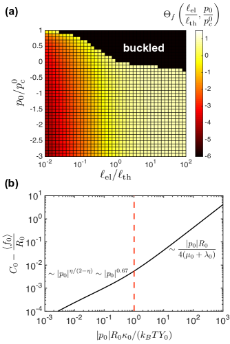
Figure 4: (Color online) Heat map depicting the average thermal shrinking of the shell radius $\left<f_{0}\right>$, as described by the scaling function $\Theta_{f}\left(\ell_{\textrm{el}}/\ell_{\textrm{th}},p_{0}/p_{c}^{0}\right)$ [see Eq. (36)]. (a) Contours of the scaling function $\Theta_{f}$ are shown with $R_{0}/\ell_{\textrm{el}}=10^{2}$, $a/R_{0}=10^{-6}$. (b) Non-linear response for large membranes ($\ell_{\textrm{th}}\ll\ell_{\textrm{el}}$) under large outward pressure $p_{0}<0$ [see Eq. (37)]. Here, the parameter on the $y$-axis $C_{0}\approx k_{B}T/(8\pi\kappa_{0})\left[\ln\left(\ell_{\textrm{th}}/a\right)+1/\eta\right]$, whereas $\ell_{\textrm{el}}/\ell_{\textrm{th}}=10^{1}$, $R_{0}/\ell_{\textrm{el}}=10^{3}$, $a/R_{0}=10^{-6}$.

Finally, we find that for large shells with $\ell_{\textrm{th}}\ll\ell_{\textrm{el}}$ that are under a stabilizing outward pressure ($p_{0}<0$), the renormalization procedure leads to a nonlinear dependence of the average shell radius shrinkage $\left<f_{0}\right>$ with internal pressure $|p_{0}|$ as (see Fig. 4b)

$$\left<f_{0}\right> \approx -\frac{|p_{0}|R_{0}^{2}}{4(\mu_{0}+\lambda_{0})}+\frac{k_{B}TR_{0}}{8\pi\kappa_{0}}\left[\ln\left(\frac{\ell_{\textrm{th}}}{a}\right)+\frac{1}{\eta}\right]$$ (37)

$$-\mathcal{C}\frac{k_{B}TR_{0}}{\kappa_{0}}\left(\frac{|p_{0}|R_{0}\kappa_{0}}{k_{B}TY_{0}}\right)^{\eta/(2-\eta)},$$

where $\mathcal{C}\approx 0.3$ and the dimensionless combination $|p_{0}|R_{0}\kappa_{0}/k_{B}TY_{0}\sim(|p_{0}|/p_{c}^{0})(\ell_{\textrm{th}}/\ell_{\textrm{el}})^{2}$. For sufficiently small outward pressures, the usual linear response term controlled by the bulk modulus $(\mu_{0}+\lambda_{0})$ is dominated by a nonlinear thermal correction $\sim|p_{0}|^{\eta/(2-\eta)}\sim|p_{0}|^{0.67}$. A similar breakdown of Hooke’s law appears in the nonlinear response to external tension for thermally fluctuation flat membranes with the same exponent $\eta/(2-\eta)$. Košmrlj and Nelson (2016) The importance of the nonlinear contribution is determined by the condition $p^{*}\lesssim 1$, where

$$p^{*}\equiv\frac{|p_{0}|R_{0}\kappa_{0}}{k_{B}TY_{0}}.$$ (38)

An alternative renormalization group matching procedure Rudnick and Nelson (1976) also exploits scaling relations such as Eq. (17), but instead integrates the recursion relations out to the intermediate scale $\ell^{*}$ defined by Eq. (32), and then matches onto perturbation theory to calculate corrections beyond that scale. We have checked that there are only order of unity differences to the results described here.

V Buckling of spherical shells

By systematically varying the bare external pressure $p_{0}$ as an initial condition in our renormalization group calculations, we identified the critical buckling pressure $p_{c}$ for spherical shells in the presence of thermal fluctuations. In agreement with the scaling description embodied in Eqs. (29) we found that the critical buckling pressure can be described with a scaling function that depends on a single dimensionless parameter

$$p_{c}=p_{c}^{0}\ \psi\!\left(\frac{\ell_{\textrm{el}}}{\ell_{\textrm{th}}}\right)=p_{c}^{0}\ \Psi\!\left(\frac{k_{B}T}{\kappa_{0}}\sqrt{\frac{Y_{0}R_{0}^{2}}{\kappa_{0}}}\right),$$ (39)

where $\Psi(x)$ is a monotonically decreasing scaling function with

$$\Psi(x) \approx \left\{\begin{array}[]{c c}1-0.28\,x^{0.4},&x\ll 1\\ -0.047\,x^{(3\eta-2)/(2+\eta)},&x\gg 1\end{array}\right..$$ (42)

The small $x$ behavior comes from a fit to our numerical calculations. The $\eta$-dependent power law $\sim-x^{0.14}$ for large $x$ matches the minimal stabilizing pressure $p_{0,\textrm{min}}$ introduced in Eq. (33). Note that thermal fluctuations lead to a substantial reduction in the critical buckling pressure $p_{c}$ and that $\Psi(x)$ becomes negative for $x\gtrsim 160$ (see Fig. 5). A remarkable consequence, is that, even when the pressure difference vanishes ($p_{0}\equiv 0$), spherical shells are only stable provided they are smaller than

$$R_{\textrm{max}}\approx 160\frac{\kappa_{0}}{k_{B}T}\sqrt{\frac{\kappa_{0}}{Y_{0}}}.$$ (43)

Larger shells are spontaneously crushed by thermal fluctuations! The condition of zero microscopic pressure difference could be achieved experimentally by studying hemispheres, which should have similar buckling thresholds to spheres, or spheres which (like wiffle balls) have a regular array of large holes.

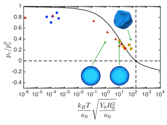
Figure 5: (Color online) Thermal fluctuations reduce critical buckling pressure $p_{c}$ below its classical value $p_{c}^{0}$ in Eq. (10), to a point where it can even assume negative values when $(k_{B}T/\kappa_{0})\sqrt{Y_{0}R_{0}^{2}/\kappa_{0}}\gg 1$. The solid black line corresponds to the theoretical prediction based on renormalization group calculations and symbols are buckling transitions extracted from the Monte Carlo simulations of Ref. Paulose et al. (2012). Green arrows point to the locations in parameter space $(k_{B}T/\kappa_{0})\sqrt{Y_{0}R_{0}^{2}/\kappa_{0}}$ and $p_{0}/p_{c}^{0}$, that correspond to the snapshots of spherical shells from the simulations shown in Fig. 1. Because for large temperatures $T$ (or equivalently for large shells $R_{0}$) the critical buckling pressure $p_{c}$ becomes negative, thermal fluctuations spontaneously crush spherical shells even at zero or somewhat negative external pressures.

The temperature-dependent critical buckling pressures obtained via numerical renormalization group methods are in reasonable agreement with the Monte Carlo simulations of Ref. Paulose et al. (2012) (see Fig. 5). Note that at small temperatures $T$ and shell sizes $R_{0}$, where we expect that the critical buckling pressure $p_{c}$ is approximately equal to the classical buckling pressure $p_{c}^{0}$, simulations show systematically lower buckling pressures. This also happens in experiments with macroscopic spherical shells, where the lower buckling pressure is due to shell imperfections Carlson et al. (1967). Similar effects could arise at low temperatures for the amorphous shells simulated in Ref. Paulose et al. (2012). Note that the temperature-dependent critical buckling pressure obtained in this paper were determined by identifying deformation modes, for which the free energy landscape becomes unstable. In practice we expect that even perfectly homogeneous thermalized spherical shells will buckle at a slightly lower external pressure, because the metastable modes embodied in a pressurized sphere exist in a shallow energy minimum, and can escape over a small energy barrier of the order $k_{B}T$ in the presence of thermal fluctuations.

VI Conclusions

In this paper we demonstrated with renormalization group methods that thermal fluctuations in thin spherical shells become significant when thermal length scale $\ell_{\textrm{th}}$ [see Eq. (19)] becomes smaller than elastic length scale $\ell_{\textrm{el}}$ [see Eq. (1)], or equivalently when $(k_{B}T/\kappa_{0})\sqrt{Y_{0}R_{0}^{2}/\kappa_{0}}\gtrsim 1$. An identical combination of variables was uncovered in the perturbation calculations of Ref. Paulose et al. (2012). If we assume that shells of thickness $h$ are constructed from a 3D isotropic elastic material with Young’s modulus $E_{0}$ and Poisson’s ratio $\nu_{0}$ [see Eq. (26)], then the relevant dimensionless parameter can be rewritten as

$$\frac{k_{B}T}{\kappa_{0}}\sqrt{\frac{Y_{0}R_{0}^{2}}{\kappa_{0}}}=\left[12(1-\nu_{0}^{2})\right]^{3/2}\frac{k_{B}TR_{0}}{E_{0}h^{4}}.$$ (44)

Thus, this critical dimensionless parameter varies as the inverse $4^{\textrm{th}}$ power of shell thickness $h$. For thermal fluctuations to become relevant at room temperature, shells only a few nanometers thick may be required. For such shells, thermal fluctuations renormalize elastic constants in the same direction as for flat solid membranes (see Eq. (25) and Figs. 3d-e), i.e. bending rigidity gets enhanced, in-plane elastic constants get reduced and all elastic constants become scale dependent. However, in striking contrast to flat membranes, where an isotropic external tension does not get renormalized, Košmrlj and Nelson (2016) thermal fluctuations can strongly enhance the effect of an inward pressure $p_{0}$. As a consequence, spherical shells get crushed at a lower external pressure than the classical zero temperature buckling pressure (see Fig. 5). In fact, shells that are larger than $R_{\textrm{max}}\approx 160(\kappa_{0}/k_{B}T)\sqrt{\kappa_{0}/Y_{0}}$ become unstable even at zero or slightly negative external pressure. Such large shells can be stabilized by a sufficiently large outward pressure $p_{0}<0$, which cuts off the renormalization of elastic constants (see Fig. 3b). We then find that the shell size increases nonlinearly with internal pressure with a universal exponent characteristic of flat membranes (see Eq. (37) and Fig. 4). Note that for sufficiently large outward pressure $p_{0}\lesssim-k_{B}TY_{0}/R_{0}\kappa_{0}$ the renormalization is completely suppressed and we recover the behavior of classical shells at zero temperature.

How do these results impact on the physics of currently available microscopic shells? Shells of microscopic organisms come in various sizes and shapes, and they need not be perfectly spherical. Therefore we just report some characteristic parameters at room temperature $T=300\textrm{K}$, where the radius $R_{0}$ is identified with half a characteristic shell diameter. For an “empty” viral capsid of bacteriophage $\phi 29$ (water inside and water outside) with $R_{0}\approx 20\textrm{-}25\textrm{nm}$, $h\approx 1.6\textrm{nm}$ and $E_{0}\approx 1.8\textrm{GPa}$, Ivanovska et al. (2004) we find that thermal fluctuations have only a small effect [$(k_{B}T/\kappa_{0})\sqrt{Y_{0}R_{0}^{2}/\kappa_{0}}\sim 0.3$]. When a capsid of bacteriophage $\phi 29$ is filled with viral DNA, the capsid is under a huge outward osmotic pressure ($p_{0}<-6\textrm{MPa}=-60\textrm{atm}$), which completely suppress thermal fluctuations [$p^{*}=|p_{0}|R_{0}\kappa_{0}/(k_{B}TY_{0})\sim 7$, see Eq. (38)]. For gram-positive bacteria, which have thick cell wall, thermal fluctuations can be ignored, e.g. for Bacillus subtilis with $R_{0}\approx 0.4\mu\textrm{m}$, $h\approx 30\textrm{nm}$, $E_{0}\approx 10\textrm{-}50\textrm{MPa}$ Amir et al. (2014) we obtain $(k_{B}T/\kappa_{0})\sqrt{Y_{0}R_{0}^{2}/\kappa_{0}}\sim 10^{-3}$. For gram-negative bacteria with thin cell walls one might think that thermal fluctuations could be important, e.g. for Escherichia coli with $R_{0}\approx 0.4\mu\textrm{m}$, $h\approx 4\textrm{nm}$, $E_{0}\approx 30\textrm{MPa}$ Amir et al. (2014) we obtain $(k_{B}T/\kappa_{0})\sqrt{Y_{0}R_{0}^{2}/\kappa_{0}}\sim 8$. However, bacteria are under a large outward osmotic stress called turgor pressure, which completely suppresses thermal fluctuations, e.g. for E. coli $p_{0}\approx-0.3\textrm{MPa}=-3\textrm{atm}$ Amir et al. (2014) and dimensionless pressure is $p^{*}=|p_{0}|R_{0}\kappa_{0}/(k_{B}TY_{0})\sim 40\gg 1$. Note that bacteria regulate osmotic pressure via mechanosensitive channels and hence, they might have evolved to the regime with large turgor pressure in order to protect their cell walls from thermal fluctuations. Somewhat similar to bacteria are nuclei in eukaryotic cells, where genetic material is protected by a nuclear envelope with $R_{0}\approx 8\mu\textrm{m}$, $h/R_{0}\sim 10^{-3}\textrm{--}10^{-2}$ and $E_{0}\sim 10^{2}\textrm{--}10^{4}\textrm{Pa}$, Kim et al. (2015) such that $(k_{B}T/\kappa_{0})\sqrt{Y_{0}R_{0}^{2}/\kappa_{0}}\sim 10^{1}\textrm{--}10^{7}$. When cells are attached to a substrate, densely packed genetic material generates a large outward osmotic pressure $p_{0}/E_{0}\approx-8\times 10^{-2}$, which suppresses thermal fluctuations ($p^{*}=|p_{0}|R_{0}\kappa_{0}/(k_{B}TY_{0})\sim 3\textrm{--}300$). However, upon detachment of cells from the substrate, the cell volume shrinks due to the release of traction forces and the resulting cytoplasm osmotic pressure crushes cell nuclei, Kim et al. (2015) a phenomenon that could be influenced by thermal fluctuations.

Thermal fluctuations definitely play an important role in red blood cell membranes. The red blood cell membrane is composed of lipid bilayer with bending rigidity $\kappa_{0}\approx 6\textrm{-}40k_{B}T$ Park et al. (2010); Evans (1983) and an attached spectrin network, which contributes to a Young’s modulus $Y_{0}\approx 25\mu\textrm{N}/\textrm{m}$ Waugh and Evans (1979); Park et al. (2010), which gives the composite system a resistance to shear. For a characteristic size of $R_{0}\approx 7\mu\textrm{m}$ we find $(k_{B}T/\kappa_{0})\sqrt{Y_{0}R_{0}^{2}/\kappa_{0}}\approx 2\textrm{-}40$. We neglect here interesting nonequilibrium effects in living cells, where ATP can be burned to turn spectrin into an “active” material. Turlier et al. (2016) Note that by treating red blood cells with mild detergents, which lyse the cells, one can produce red blood cell “ghosts” that are composed of spectrin skeleton alone. Such membranes have smaller bending rigidity and exhibit much larger fluctuations, which was used to confirm the scale-dependence of elastic constants via X-ray and light scattering experiments in Ref. Schmidt et al. (1993).

As discussed in Ref. Paulose et al. (2012), artificial microscopic shells have also been constructed from polyelectrolytes Elsner et al. (2006), proteins Hermanson et al. (2007) and polymers Shum et al. (2008). Such microcapsules can be made extremely thin, with the thickness of several nanometers, where thermal fluctuations can become relevant. For example, microcapsules with $h\approx 6\textrm{nm}$ thickness were fabricated from reconstituted spider silk Hermanson et al. (2007) with $R_{0}\approx 30\mu\textrm{m}$ and $E_{0}\approx 1\textrm{GPa}$, where we find $(k_{B}T/\kappa_{0})\sqrt{Y_{0}R_{0}^{2}/\kappa_{0}}\sim 3$. Similar polymersomes can be made 10 times larger with $R_{0}\approx 300\mu{\textrm{m}}$, while being thinner than 10 nanometers. Shum et al. (2008) Polycrystalline shells or hemispheres of graphene provide a particularly promising candidate for observing the effects of thermal fluctuations on solid membranes with a spherical background curvature. Indeed, with graphene parameters ($\kappa_{0}=1.1\textrm{eV}$ Fasolino et al. (2007) and $Y_{0}=340\textrm{N}/\textrm{m}$ Lee et al. (2008)), the maximum allowed radius when $p_{0}=0$ at room temperature from Eq. (43) is $R_{\textrm{max}}\approx 160\textrm{nm}$. We hope this paper will stimulate further experimental and numerical investigations of the stability and mechanical properties of thermalized spheres.

Appendix A Renormalization group recursion relations for spherical shells

In this Appendix we derive the renormalization group recursion relations displayed in Eqs. (15). We start by rewriting the free energy in Eq. (7) in Fourier space as

$$F_{\textrm{eff}} = F_{0}+F_{\textrm{int}},$$ (45a)

$$\frac{F_{0}}{A} = \sum_{\bf q}\frac{1}{2}\left[\kappa_{0}q^{4}-\frac{p_{0}R_{0}q^{2}}{2}+\frac{Y_{0}}{R_{0}^{2}}\right]\tilde{f}({\bf q})\tilde{f}(-{\bf q})$$ (45b)

$$\frac{F_{\textrm{int}}}{A} = \sum_{\begin{subarray}{c}{\bf q}_{1}+{\bf q}_{2}={\bf q}\neq{\bf 0}\\ {\bf q}_{3}+{\bf q}_{4}=-{\bf q}\neq{\bf 0}\end{subarray}}\frac{Y_{0}}{8}\left[q_{1i}P_{ij}^{T}({\bf q})q_{2j}\right]\left[q_{3i}P_{ij}^{T}({\bf q})q_{4j}\right]$$

$$\quad\quad\quad\quad\quad\quad\quad\times\tilde{f}({\bf q}_{1})\tilde{f}({\bf q}_{2})\tilde{f}({\bf q}_{3})\tilde{f}({\bf q}_{4})$$

$$+\!\!\!\!\sum_{\begin{subarray}{c}{\bf q}_{1}\neq{\bf 0}\\ {\bf q}_{2}+{\bf q}_{3}=-{\bf q}_{1}\end{subarray}}\!\!\!\!\frac{Y_{0}}{2R_{0}}\left[q_{2i}P_{ij}^{T}({\bf q}_{1})q_{3j}\right]\tilde{f}({\bf q}_{1})\tilde{f}({\bf q}_{2})\tilde{f}({\bf q}_{3}),$$

where $A$ is the area, $\tilde{f}({\bf q})=\int(d^{2}{\bf r}/A)e^{-i{\bf q}\cdot{\bf r}}\tilde{f}({\bf r})$, and $P_{ij}^{T}({\bf q})=\delta_{ij}-q_{i}q_{j}/q^{2}$ is the transverse projection operator. Note that the sums over wavevectors can be converted to integrals in the shallow-shell approximation as $\sum_{\bf q}\rightarrow A\int\!d^{2}{\bf q}/(2\pi)^{2}$.

To implement the momentum shell renormalization group, we first integrate out all Fourier modes in a thin momentum shell $\Lambda/b<q<\Lambda$, where $a=\pi/\Lambda$ is a microscopic cutoff and $b=e^{s}$ with $s\ll 1$. Next we rescale lengths and fields Aronovitz and Lubensky (1988); Radzihovsky and Nelson (1991)

$${\bf r} = b{\bf r}^{\prime},$$ (46a)

$${\bf q} = b^{-1}{\bf q}^{\prime},$$ (46b)

$$\tilde{f}({\bf q}) = b^{\zeta_{f}}\tilde{f}^{\prime}({\bf q}^{\prime}),$$ (46c)

where the field rescaling exponent $\zeta_{f}$ will be chosen to simplify the resulting renormalization group equations. Finally, we define new elastic constants $\kappa^{\prime}$, $Y^{\prime}$, and external pressure $p^{\prime}$, such that the free energy functional in Eq. (45) retains the same form after the first two renormalization group steps.

The integration of Fourier modes in a thin momentum shell $\Lambda/b<k<\Lambda$ is formally done with a functional integral

$$F_{\textrm{eff}}^{\prime}[\{{\bf q}\}]\! = \!-k_{B}T\ln\!\!\left[\!\int\!\!\mathcal{D}[\tilde{f}({\bf k})]e^{-(F_{0}[\{{\bf q},{\bf k}\}]+F_{\textrm{int}}[\{{\bf q},{\bf k}\}])/k_{B}T}\right],$$

$$F_{\textrm{eff}}^{\prime}[\{{\bf q}\}] = F_{\textrm{0}}[\{{\bf q}\}]-k_{B}T\ln\left<e^{-F_{\textrm{int}}[\{{\bf q},{\bf k}\}]/k_{B}T}\right>_{0,{\bf k}},$$ (47)

where $q<\Lambda/b$ and we introduced the average

$$\left<\mathcal{O}\right>_{0,{\bf k}}=\frac{\int\mathcal{D}[\tilde{f}({\bf k})]\mathcal{O}e^{-F_{0}[\{{\bf k}\}]}}{\int\mathcal{D}[\tilde{f}({\bf k})]e^{-F_{0}[\{{\bf k}\}]}}.$$ (48)

The term involving a logarithm in Eq. (47) can be expanded in terms of the cumulants

$$F_{\textrm{eff}}^{\prime}[\{{\bf q}\}]\!=\!F_{\textrm{0}}[\{{\bf q}\}]+\sum_{n}\frac{(-1)^{n-1}}{n!(k_{B}T)^{n-1}}\bigg{<}\big{(}F_{\textrm{int}}[\{{\bf q},{\bf k}\}]\big{)}^{n}\bigg{>}^{(c)}_{0,{\bf k}},$$ (49)

where $\langle\mathcal{O}\rangle^{(c)}=\langle\mathcal{O}\rangle$, $\langle\mathcal{O}^{2}\rangle^{(c)}=\langle\mathcal{O}^{2}\rangle-\langle\mathcal{O}\rangle^{2}$, etc. The infinite series in Eq. (49) above can be systematically approximated with Feynman diagrams Amit and Mayor (2005); Fig. 2 displays all relevant diagrams to one loop order. The contributions of the diagrams in Fig. 2c-i are

$$\frac{F_{\textrm{eff}}^{\prime}[\{{\bf q}\}]_{(c)}}{A} = \sum_{\bf q}\frac{1}{2}\tilde{f}({\bf q})\tilde{f}(-{\bf q})\int_{\Lambda/b<|{\bf k}|<\Lambda}\frac{d^{2}{\bf k}}{(2\pi)^{2}}AYG_{ff}\left({\bf k}+\frac{\bf q}{2}\right)\left[q_{i}P^{T}_{ij}\left({\bf k}-\frac{\bf q}{2}\right)\big{(}k_{j}+\frac{q_{j}}{2}\big{)}\right]^{2},$$ (50a)

$$\frac{F_{\textrm{eff}}^{\prime}[\{{\bf q}\}]_{(d-g)}}{A} = \sum_{\bf q}\frac{1}{2}\tilde{f}({\bf q})\tilde{f}(-{\bf q})\int_{\Lambda/b<|{\bf k}|<\Lambda}\frac{d^{2}{\bf k}}{(2\pi)^{2}}\frac{(-1)Y^{2}A^{2}}{k_{B}TR^{2}}G_{ff}\left({\bf k}+\frac{\bf q}{2}\right)G_{ff}\left({\bf k}-\frac{\bf q}{2}\right)$$

$$\quad\times\left\{\left[q_{i}P^{T}_{ij}\left({\bf k}+\frac{\bf q}{2}\right)\big{(}k_{j}-\frac{q_{j}}{2}\big{)}\right]^{2}-\left[q_{i}P^{T}_{ij}\left({\bf k}-\frac{\bf q}{2}\right)\big{(}k_{j}+\frac{q_{j}}{2}\big{)}\right]\left[q_{i}P^{T}_{ij}\left({\bf k}+\frac{\bf q}{2}\right)\big{(}k_{j}-\frac{q_{j}}{2}\big{)}\right]\right.$$

$$\quad\quad\left.+2\left[q_{i}P^{T}_{ij}\left({\bf k}-\frac{\bf q}{2}\right)\big{(}k_{j}+\frac{q_{j}}{2}\big{)}\right]\left[\big{(}k_{i}-\frac{q_{i}}{2}\big{)}P^{T}_{ij}\left({\bf q}\right)\big{(}k_{j}+\frac{q_{j}}{2}\big{)}\right]+\frac{1}{2}\left[\big{(}k_{i}-\frac{q_{i}}{2}\big{)}P^{T}_{ij}\left({\bf q}\right)\big{(}k_{j}+\frac{q_{j}}{2}\big{)}\right]^{2}\right\},$$

$$\frac{F_{\textrm{eff}}^{\prime}[\{{\bf q}\}]_{(h)}}{A} = \sum_{\begin{subarray}{c}{\bf q}\neq{\bf 0}\\ {\bf q}_{2}+{\bf q}_{3}=-{\bf q}\end{subarray}}\frac{Y}{2R}\left[q_{2i}P_{ij}^{T}({\bf q})q_{3j}\right]\tilde{f}({\bf q})\tilde{f}({\bf q}_{2})\tilde{f}({\bf q}_{3})$$ (50c)

$$\quad\quad\times\int_{\Lambda/b<|{\bf k}|<\Lambda}\frac{d^{2}{\bf k}}{(2\pi)^{2}}\frac{(-1)YA^{2}}{2k_{B}T}G_{ff}\left({\bf k}+\frac{{\bf q}}{2}\right)G_{ff}\left({\bf k}-\frac{{\bf q}}{2}\right)\left[\big{(}k_{i}-\frac{q_{i}}{2}\big{)}P^{T}_{ij}\left({\bf q}\right)\big{(}k_{j}+\frac{q_{j}}{2}\big{)}\right]^{2},$$

$$\frac{F_{\textrm{eff}}^{\prime}[\{{\bf q}\}]_{(i)}}{A} = \sum_{\begin{subarray}{c}{\bf q}_{1}+{\bf q}_{2}={\bf q}\neq{\bf 0}\\ {\bf q}_{3}+{\bf q}_{4}=-{\bf q}\neq{\bf 0}\end{subarray}}\frac{Y}{8}\left[q_{1i}P_{ij}^{T}({\bf q})q_{2j}\right]\left[q_{3i}P_{ij}^{T}({\bf q})q_{4j}\right]\tilde{f}({\bf q}_{1})\tilde{f}({\bf q}_{2})\tilde{f}({\bf q}_{3})\tilde{f}({\bf q}_{4})$$ (50d)

$$\quad\quad\times\int_{\Lambda/b<|{\bf k}|<\Lambda}\frac{d^{2}{\bf k}}{(2\pi)^{2}}\frac{(-1)YA^{2}}{2k_{B}T}G_{ff}\left({\bf k}+\frac{{\bf q}}{2}\right)G_{ff}\left({\bf k}-\frac{{\bf q}}{2}\right)\left[\big{(}k_{i}-\frac{q_{i}}{2}\big{)}P^{T}_{ij}\left({\bf q}\right)\big{(}k_{j}+\frac{q_{j}}{2}\big{)}\right]^{2},$$

where $G_{ff}({\bf q})=k_{B}T/[A(\kappa q^{4}-pRq^{2}/2+Y/R^{2})]$, and subscripts $(c)$, $(d-g)$, $(h)$ and $(i)$ describe contributions from the corresponding diagrams in Fig. 2. The integrands in the equations above must now be expanded for small wavevectors ${\bf q}$. The relevant contributions to $\kappa^{\prime}$, $p^{\prime}$ and $Y^{\prime}$ are related to terms that scale with $q^{4}$, $q^{2}$ and $q^{0}$ in Eqs. (50a) and (LABEL:eq:app:2), respectively. The contributions to three-point and four-point vertices are described with Eqs. (50c) and (50d), respectively, and here it is enough to keep only the $q^{0}$ terms in the integrands.

After the integration of Fourier modes in a thin momentum shell $\Lambda/b<k<\Lambda$, where $b=e^{s}$ with $s\gg 1$, rescaling fields, momenta and lengths according to Eq. (46) we find the recursion relations

$$\beta_{\kappa} = \frac{d\kappa^{\prime}}{ds}=2(\zeta_{f}-1)\kappa^{\prime}+\frac{3k_{B}TY^{\prime}\Lambda^{2}}{16\pi\mathcal{D}}-\frac{3k_{B}TY^{\prime 2}\Lambda^{2}}{8\pi R^{\prime 2}\mathcal{D}^{2}}\bigg{[}1+\frac{I_{\kappa 1}}{\mathcal{D}^{2}}+\frac{I_{\kappa 2}}{\mathcal{D}^{4}}\bigg{]},$$ (51a)

$$\beta_{Y} = \frac{dY^{\prime}}{ds}=2\zeta_{f}Y^{\prime}-\frac{3k_{B}TY^{\prime 2}\Lambda^{6}}{32\pi\mathcal{D}^{2}},$$ (51b)

$$\beta_{p} = \frac{dp^{\prime}}{ds}=(2\zeta_{f}+1)p^{\prime}+\frac{3k_{B}TY^{\prime 2}\Lambda^{4}}{4\pi R^{\prime 3}\mathcal{D}^{2}}\left[1+\frac{I_{p}}{\mathcal{D}^{2}}\right],\quad\$$ (51c)

$$\beta_{R} = \frac{dR^{\prime}}{ds}=-R^{\prime},$$ (51d)

where we introduce a denominator factor $\mathcal{D}$ and the results of various integrations as

$$\mathcal{D} = \kappa^{\prime}\Lambda^{4}-\frac{p^{\prime}R^{\prime}\Lambda^{2}}{2}+\frac{Y^{\prime}}{R^{\prime 2}},$$ (52a)

$$I_{\kappa 1} = \frac{1}{48}\bigg{[}-\frac{4Y^{\prime 2}}{R^{\prime 4}}+8\frac{Y^{\prime}}{R^{\prime 2}}\left(2p^{\prime}R^{\prime}\Lambda^{2}-9\kappa^{\prime}\Lambda^{4}\right)-\left(5p^{\prime 2}R^{\prime 2}\Lambda^{4}-32p^{\prime}R^{\prime}\kappa\Lambda^{6}+36\kappa^{\prime 2}\Lambda^{8}\right)\bigg{]},$$ (52b)

$$I_{\kappa 2} = \frac{1}{768}\bigg{[}-\frac{24Y^{\prime 3}\kappa^{\prime}\Lambda^{4}}{R^{\prime 6}}+\frac{Y^{\prime 2}}{R^{\prime 4}}\big{(}9p^{\prime 2}R^{\prime 2}\Lambda^{4}-76p^{\prime}R^{\prime}\kappa^{\prime}\Lambda^{6}+268\kappa^{\prime 2}\Lambda^{8}\big{)}$$ (52c)

$$\quad\quad+\frac{Y^{\prime}}{R^{\prime 2}}\big{(}-5p^{\prime 3}R^{\prime 3}\Lambda^{6}+52p^{\prime 2}R^{\prime 2}\kappa^{\prime}\Lambda^{8}-204p^{\prime}R^{\prime}\kappa^{\prime 2}\Lambda^{10}+160\kappa^{\prime 3}\Lambda^{12}\big{)}$$

$$\quad\quad+\big{(}p^{\prime 4}R^{\prime 4}\Lambda^{8}-12p^{\prime 3}R^{\prime 3}\kappa^{\prime}\Lambda^{10}+56p^{\prime 2}R^{\prime 2}\kappa^{\prime 2}\Lambda^{12}-96p^{\prime}R^{\prime}\kappa^{\prime 3}\Lambda^{14}+60\kappa^{\prime 4}\Lambda^{16}\big{)}\bigg{]},$$

$$I_{p} = \frac{1}{48}\bigg{[}\frac{Y}{R^{2}}\big{(}3p^{\prime}R^{\prime}\Lambda^{2}-16\kappa^{\prime}\Lambda^{4}\big{)}+\big{(}-p^{\prime 2}R^{\prime 2}\Lambda^{4}+7p^{\prime}R^{\prime}\kappa^{\prime}\Lambda^{6}-8\kappa^{\prime 2}\Lambda^{8}\big{)}\bigg{]}.$$ (52d)

The $\beta_{Y}$ recursion relation in Eq. (51b) describes changes in the quadratic “mass” proportional to $Y$ in Eq. (45). Similarly, we can calculate the recursion relations for the cubic and quartic terms in Eq. (45). The only significant change is in the effect of rescaling: the $2\zeta_{f}Y$ term now becomes $(3\zeta_{f}-1)Y$ and $(4\zeta_{f}-2)Y$, respectively.

Appendix B Independence of renormalization group results on the choice of $\zeta_{f}$

In this section we illustrate the insensitivity of the renormalization procedure to the precise choice of the field rescaling factor that appears in $\tilde{f}({\bf q})=b^{\zeta_{f}}\tilde{f}^{\prime}({\bf q}^{\prime})$. Specifically we demonstrate that for a flat thermalized sheet we show that the renormalized bending rigidity $\kappa_{R}(\ell)$ and renormalized Young’s modulus $Y_{R}(\ell)$ are identical, when we chose either $\zeta_{f}(s)\equiv 1$, as we did for convenience with spherical shells, or we choose $\zeta_{f}(s)$ such that the the $\kappa^{\prime}(\ell)\equiv\kappa_{0}$ remains fixed, as is the case in the usual renormalization group procedure. Radzihovsky and Nelson (1991)

The recursion relations for flat sheets are Radzihovsky and Nelson (1991); Košmrlj and Nelson (2016)

$$\beta_{\kappa} = \frac{d\kappa^{\prime}}{ds}=2(\zeta_{f}-1)\kappa^{\prime}+\frac{3k_{B}TY^{\prime}}{16\pi\kappa^{\prime}\Lambda^{2}},$$ (53a)

$$\beta_{Y} = \frac{dY^{\prime}}{ds}=(4\zeta_{f}-2)Y^{\prime}-\frac{3k_{B}TY^{\prime 2}}{32\pi\kappa^{\prime 2}\Lambda^{2}}.$$ (53b)

The scale-dependent parameters $\kappa^{\prime}(s)$, $Y^{\prime}(s)$, which are obtained by integrating the differential equations in Eqs. (57) up to $s=\ln(\ell/a)$ with initial conditions $\kappa^{\prime}(0)=\kappa_{0}$, $Y^{\prime}(0)=Y_{0}$, are related to the scaling of propagator $G_{ff}(q)$ according to Amit and Mayor (2005)

$$G_{ff}(q|\kappa_{0},A)=e^{\int\!2\zeta_{f}(s)ds}G_{ff}(qe^{s}|\kappa^{\prime}(s),Ae^{-2s}),$$ (54)

where $G_{ff}(q|\kappa,A)=k_{B}T/[A\kappa q^{4}]$ and we explicitly wrote the rescaled momenta $q^{\prime}=qe^{s}$ and the rescaled patch area $A^{\prime}=Ae^{-2s}$. By replacing the left hand side in the Eq. (54) above with the propagator $G_{ff}(q)=k_{B}T/[A(\kappa_{R}(q)q^{4})]$, we find the renormalized bending rigidity

$$\kappa_{R}(s) = \kappa^{\prime}(s)e^{\int[2-2\zeta_{f}(s)]ds}.$$ (55)

From a similar scaling relation for the four-point vertex we find

$$Y_{R}(s) = Y^{\prime}(s)e^{\int[2-4\zeta_{f}(s)]ds}.$$ (56)

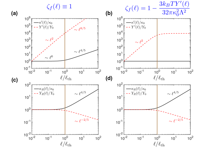
Figure 6: (Color online) Renormalization group flows in thermalized flat sheets with $a/\ell_{\textrm{th}}=10^{-2}$ for two different choices of scaling exponents $\zeta_{f}$. Plots on the left correspond to $\zeta_{f}(\ell)\equiv 1$ and plots on the right correspond to $\zeta_{f}(\ell)=1-3k_{B}TY^{\prime}(\ell)/(32\pi\kappa_{0}^{2}\Lambda^{2})$, which fixes $\kappa^{\prime}(\ell)\equiv\kappa_{0}$. (a-b) Renormalization group flows for $\kappa^{\prime}(\ell)$ and $Y^{\prime}(\ell)$ obtained (a) from Eq. (57) and (b) from Eq. (60a). (c-d) Scale dependence of renormalized elastic constants $\kappa_{R}(\ell)$ and $Y_{R}(\ell)$ obtained by removing the scaling factors from $\kappa^{\prime}(\ell)$ and $Y^{\prime}(\ell)$ as described in Eqs. (55) and (56). Note that the physical renormalized constants $\kappa_{R}(\ell)$ and $Y_{R}(\ell)$ are identical in (c) and (d), even though the flows of $\kappa^{\prime}(\ell)$ and $Y^{\prime}(\ell)$ in (a) and (b) depend on the precise choice of the scaling exponent $\zeta_{f}(\ell)$.

First we choose $\zeta_{f}(s)\equiv 1$, which leads to the recursion relations to

$$\frac{d\kappa^{\prime}}{ds} = \frac{3k_{B}TY^{\prime}}{16\pi\kappa^{\prime}\Lambda^{2}},$$ (57a)

$$\frac{dY^{\prime}}{ds} = 2Y^{\prime}-\frac{3k_{B}TY^{\prime 2}}{32\pi\kappa^{\prime 2}\Lambda^{2}}.$$ (57b)

By integrating the differential equations in Eqs. (57) up to $s=\ln(\ell/a)$ with initial conditions $\kappa^{\prime}(0)=\kappa_{0}$ and $Y^{\prime}(0)=Y_{0}$ we find (see Fig. 6)

$$\kappa^{\prime}(\ell) \sim \left\{\begin{array}[]{c c}\kappa_{0},&\ell\ll\ell_{\textrm{th}}\\ \ \ \quad\kappa_{0}(\ell/\ell_{\textrm{th}})^{4/5},&\ell\gg\ell_{\textrm{th}}\end{array}\right.,$$ (58c)

$$Y^{\prime}(\ell) \sim \left\{\begin{array}[]{c c}Y_{0}(\ell/a)^{2},&\ell\ll\ell_{\textrm{th}}\\ Y_{0}(\ell_{\textrm{th}}/a)^{2}(\ell/\ell_{\textrm{th}})^{8/5},&\ell\gg\ell_{\textrm{th}}\end{array}\right.,$$ (58f)

where $\ell_{\textrm{th}}\sim\kappa_{0}/\sqrt{k_{B}TY_{0}}$. Upon removing scaling factors according to Eqs. (55) and (56) we obtain our final scale-dependent renormalized elastic constants

$$\kappa_{R}(\ell) \sim \left\{\begin{array}[]{c c}\kappa_{0},&\ell\ll\ell_{\textrm{th}}\\ \ \kappa_{0}(\ell/\ell_{\textrm{th}})^{4/5},&\ell\gg\ell_{\textrm{th}}\end{array}\right.,$$ (59c)

$$Y_{R}(\ell) \sim \left\{\begin{array}[]{c c}Y_{0},&\ell\ll\ell_{\textrm{th}}\\ Y_{0}(\ell/\ell_{\textrm{th}})^{-2/5},&\ell\gg\ell_{\textrm{th}}\end{array}\right.,$$ (59f)

where we recognize the usual scaling exponents $\eta=4/5$ and $\eta_{u}=2/5$, which satisfy identity $\eta_{u}+2\eta=2$.

A more conventional choice, Radzihovsky and Nelson (1991); Aronovitz and Lubensky (1988) is to take $\zeta_{f}(s)$ such that the $\kappa^{\prime}(s)\equiv\kappa_{0}$ remains fixed. Upon setting $\beta_{\kappa}=0$ in Eq. (53a) we find

$$\zeta_{f}(s) = 1-\frac{3k_{B}TY^{\prime}(s)}{32\pi\kappa_{0}^{2}\Lambda^{2}}$$ (60a)

$$\frac{dY^{\prime}(s)}{ds} = 2Y^{\prime}(s)-\frac{15k_{B}TY^{\prime}(s)^{2}}{32\pi\kappa_{0}^{2}\Lambda^{2}},$$ (60b)

By integrating the differential equations in Eqs. (60a) up to $s=\ln(\ell/a)$ with initial condition $Y^{\prime}(0)=Y_{0}$ we find a fixed point, which is reached at the thermal scale, $\ell\sim\ell_{\textrm{th}}$ (see Fig. 6) such that

$$\zeta_{f}(\ell) \sim \left\{\begin{array}[]{c c}1,&\ell\ll\ell_{\textrm{th}}\\ \quad\quad\frac{3}{5},&\ell\gg\ell_{\textrm{th}}\end{array}\right.,$$ (61c)

$$Y^{\prime}(\ell) \sim \left\{\begin{array}[]{c c}Y_{0}(\ell/a)^{2},&\ell\ll\ell_{\textrm{th}}\\ \ \ \frac{64\pi\kappa_{0}^{2}\Lambda^{2}}{15k_{B}T},&\ell\gg\ell_{\textrm{th}}\end{array}\right..$$ (61f)

By taking into account scaling factors in Eqs. (55) and (56), it is easy to see that the value of exponent $\zeta_{f}^{*}=3/5$ at the fixed point leads to the scaling exponents $\eta=2-2\zeta_{f}^{*}=4/5$ and $\eta_{u}=4\zeta_{f}^{*}-2=2/5$. From these relations one also finds the identity $\eta_{u}+2\eta=2$ regardless of the precise value of $\zeta_{f}^{*}$. From Fig. (6) we see that the renormalized bending rigidity $\kappa_{R}(\ell)$ and the renormalized Young’s modulus $Y_{R}(\ell)$ are identical to the ones obtained in Eq. (59) with the choice of $\zeta(s)\equiv 1$.

References

- Love (1888) A. E. H. Love, “The small free vibrations and deformation of a thin elastic shell,” Phil. Trans. R. Soc. Lond. A 179, 491–546 (1888).
- Föppl (1907) A. Föppl, “Vorlesungen über technische mechanik,” B.G. Teubner 5, 132 (1907).
- von Kármán (1910) T. von Kármán, “Festigkeitsproblem im maschinenbau,” Encyk. D. Math. Wiss. 4, 311–385 (1910).
- Sanders (1963) J. L. Sanders, “Nonlinear theories of thin shells,” Q. Appl. Math. 21, 21–36 (1963).
- Koiter (1966) W. T. Koiter, “On the nonlinear theory of thin elastic shells,” Proc. K. Ned. Akad. Wet. B 69, 1–54 (1966).
- Krieger (2012) K. Krieger, “Extreme mechanics: Buckling down,” Nature 488, 146–147 (2012).
- Stoop et al. (2015) N. Stoop, R. Lagrange, D. Terwagne, P. M. Reis, and J. Dunkel, “Curvature-induced symmetry breaking determines elastic surface patterns,” Nat. Mater. 14, 337–342 (2015).
- Lidmar et al. (2003) J. Lidmar, L. Mirny, and D. R. Nelson, “Virus shapes and buckling transitions in spherical shells,” Phys. Rev. E 68, 051910 (2003).
- Ivanovska et al. (2004) I. L. Ivanovska, P. J. de Pablo, B. Ibarra, G. Sgalari, F. C. MacKintosh, J. L. Carrascosa, C. F. Schmidt, and G. J. L. Wuite, “Bacteriophage capsids: Tough nanoshells with complex elastic properties,” Proc. Natl. Acad. Sci. USA 101, 7600–7605 (2004).
- Michel et al. (2006) J. P. Michel, I. L. Ivanovska, M. M. Gibbons, W. S. Klug, C. M. Knobler, G. J. L. Wuite, and C. F. Schmidt, “Nanoindentation studies of full and empty viral capsids and the effects of capsid protein mutations on elasticity and strength,” Proc. Natl. Acad. Sci. USA 103, 6184–6189 (2006).
- Klug et al. (2006) W. S. Klug, R. F. Bruinsma, J.-P. Michel, C. M. Knobler, I. L. Ivanovska, C. F. Schmidt, and G. J. L. Wuite, “Failure of viral shells,” Phys. Rev. Lett. 97, 228101 (2006).
- Yao et al. (1999) X. Yao, M. Jericho, D. Pink, and T. Beveridge, “Thickness and elasticity of gram-negative murein sacculi measured by atomic force microscopy,” J. Bacteriol. 181, 6865–75 (1999).
- Wang et al. (2010) S. Wang, H. Arellano-Santoyo, P. A. Combs, and J. W. Shaevitz, “Actin-like cytoskeleton filaments contribute to cell mechanics in bacteria,” Proc. Natl. Acad. Sci. USA 107, 9182–9185 (2010).
- Nelson (2012) D. R. Nelson, “Biophysical dynamics in disorderly environments,” Annu. Rev. Biophys. 41, 371–402 (2012).
- Amir et al. (2014) A. Amir, F. Babaeipour, D. B. McIntosh, D. R. Nelson, and S. Jun, “Bending forces plastically deform growing bacterial cell walls,” Proc. Natl. Acad. Sci. USA 111, 5778–5783 (2014).
- Waugh and Evans (1979) R. Waugh and E. A. Evans, “Thermoelasticity of red blood cell membrane,” Biophys J. 26, 115–131 (1979).
- Evans (1983) E. A. Evans, “Bending elastic modulus of red blood cell membrane derived from buckling instability in micropipet aspiration tests.” Biophys J. 43, 27–30 (1983).
- Park et al. (2010) Y. Park, C. A. Best, K. Badizadegan, R. R. Dasari, M. S. Feld, T. Kuriabova, M. L. Henle, A. J. Levine, and G. Popescu, “Measurement of red blood cell mechanics during morphological changes,” Proc. Natl. Acad. Sci. USA 107, 6731–6736 (2010).
- Gao et al. (2001) C. Gao, E. Donath, S. Moya, V. Dudnik, and H. Möhwald, “Elasticity of hollow polyelectrolyte capsules prepared by the layer-by-layer technique,” Eur. Phys. J. E 5, 21–27 (2001).
- Gordon et al. (2004) V. D. Gordon, X. Chen, J. W. Hutchinson, A. R. Bausch, M. Marquez, and D. A. Weitz, “Self-assembled polymer membrane capsules inflated by osmotic pressure,” J. Am. Chem. Soc. 126, 14117–14122 (2004).
- Lulevich et al. (2004) V. V. Lulevich, D. Andrienko, and O. I. Vinogradova, “Elasticity of polyelectrolyte multilayer microcapsules,” J. Chem. Phys. 120, 3822 (2004).
- Elsner et al. (2006) N. Elsner, F. Dubreuil, R. Weinkamer, M. Wasicek, F. D. Fischer, and A. Fery, “Mechanical properties of freestanding polyelectrolyte capsules: a quantitative approach based on shell theory,” Progr. Colloid Polym. Sci. 132, 117–123 (2006).
- Zoldesi et al. (2008) C. I. Zoldesi, I. L. Ivanovska, C. Quilliet, G. J. L. Wuite, and A. Imhof, “Elastic properties of hollow colloidal particles,” Phys. Rev. E 78, 051401 (2008).
- de Gennes (1979) P.-G. de Gennes, Scaling Concepts in Polymer Physics (Cornell University Press, Ithaca, 1979).
- Doi and Edwards (1986) M. Doi and S. F. Edwards, The Theory of Polymer Dynamics (Clarendon Press, Oxford, 1986).
- Nelson and Peliti (1987) D. R. Nelson and L. Peliti, “Fluctuations in membranes with crystalline and hexatic order,” J. Phys. (France) 48, 1085 (1987).
- Nelson et al. (2004) D. R. Nelson, T. Piran, and S. Weinberg, eds., Statistical Mechanics of Membranes and Surfaces, 2nd ed. (World Scientific, Singapore, 2004).
- Katsnelson (2012) M. I. Katsnelson, Graphene : Carbon in Two Dimensions (Cambridge University Press, New York, 2012).
- Schmidt et al. (1993) C. F. Schmidt, K. Svoboda, N. Lei, I. B. Petsche, L. E. Berman, C. R. Safinya, and G. S. Grest, “Existence of a flat phase in red cell membrane skeletons,” Science 259, 952–955 (1993).
- Novoselov et al. (2005) K. S. Novoselov, D. Jiang, F. Schedin, T. J. Booth, V. V. Khotkevich, S. V. Morozov, and A. K. Geim, “Two-dimensional atomic crystals.” Proc. Natl. Acad. Sci. USA 102, 10451–10453 (2005).
- Blees et al. (2015) M. K. Blees, A. W. Barnard, P. A. Rose, S. P. Roberts, K. L. McGill, P. Y. Huang, A. R. Ruyack, J. W. Kevek, B. Kobrin, D. A. Muller, and P. L. McEuen, “Graphene kirigami,” Nature 524, 204–207 (2015).
- Nicholl et al. (2015) R. J. T. Nicholl, H. J. Conley, N. V. Lavrik, I. Vlassiouk, Y. S. Puzyrev, V. P. Sreenivas, S. T. Pantelides, and K. I. Bolotin, “Mechanics of free-standing graphene: Stretching a crumpled membrane,” Nat. Comm. 6, 8789 (2015).
- Radzihovsky and Nelson (1991) L. Radzihovsky and D. R. Nelson, “Statistical-mechanics of randomly polymerized membranes,” Phys. Rev. A. 44, 3525–3542 (1991).
- Košmrlj and Nelson (2013) A. Košmrlj and D. R. Nelson, “Mechanical properties of warped membranes,” Phys. Rev. E 88, 012136 (2013).
- Košmrlj and Nelson (2014) A. Košmrlj and D. R. Nelson, “Thermal excitations of warped membranes,” Phys. Rev. E 89, 022126 (2014).
- Paulose et al. (2012) J. Paulose, G. A. Vliegenthart, G. Gompper, and D. R. Nelson, “Fluctuating shells under pressure,” Proc. Natl. Acad. Sci. USA 109, 19551–19556 (2012).
- Aronovitz and Lubensky (1988) J. A. Aronovitz and T. C. Lubensky, “Fluctuations of solid membranes,” Phys. Rev. Lett. 60, 2634–2637 (1988).
- Guitter et al. (1989) E. Guitter, F. David, S. Leibler, and L. Peliti, “Thermodynamical behavior of polymerized membranes,” J. Phys. (France) 50, 1787–1819 (1989).
- van der Heijden (2009) A. M. A. van der Heijden, ed., W. T. Koiter’s Elastic Stability of Solids and Structures (Cambridge University Press, New York, 2009).
- Phillips et al. (2013) R. Phillips, J. Kondev, J. Theriot, and H. G. Garcia, eds., Physical Biology of the Cell, 2nd ed. (Garland Science, New York, 2013).
- Landau and Lifshitz (1970) L. D. Landau and E. M. Lifshitz, Theory of Elasticity, 2nd ed. (Pergamon Press, New York, 1970).
- Hutchinson (1967) J. W. Hutchinson, “Imperfection sensitivity of externally pressurized spherical shells,” J. Appl. Mech. 34, 49–55 (1967).
- Katifori et al. (2010) E. Katifori, S. Alben, E. Cerda, D. R. Nelson, and J. Dumais, “Foldable structures and the natural design of pollen grains,” Proc. Natl. Acad. Sci. USA 107, 7635–7639 (2010).
- Le Doussal and Radzihovsky (1992) P. Le Doussal and L. Radzihovsky, “Self-consistent theory of polymerized membranes,” Phys. Rev. Lett. 69, 1209–1212 (1992).
- Amit and Mayor (2005) D. J. Amit and V. M. Mayor, Field Theory, the Renormalization Group, and Critical Phenomena: Graphs to Computers, 3rd ed. (World Scientific, Singapore, 2005).
- Košmrlj and Nelson (2016) A. Košmrlj and D. R. Nelson, “Response of thermalized ribbons to pulling and bending,” Phys. Rev. B 93, 125431 (2016).
- Roldan et al. (2011) R. Roldan, A. Fasolino, K. V. Zakharchenko, and M. I. Katsnelson, “Suppression of anharmonicities in crystalline membranes by external strain,” Phys. Rev. B. 83, 174104 (2011).
- Rudnick and Nelson (1976) J. Rudnick and D. R. Nelson, “Equations of state and renormalization-group recursion relations,” Phys. Rev. B 13, 2208 (1976).
- Carlson et al. (1967) R. L. Carlson, R. L. Sendelbeck, and N. J. Hoff, “Experimental studies of the buckling of complete spherical shells,” Exp. Mech. 7, 281–288 (1967).
- Kim et al. (2015) D.-H. Kim, B. Li, F. Si, J. M. Phillip, D. Wirtz, and S. X. Sun, “Volume regulation and shape bifurcation in the cell nucleus,” J. Cell Sci. 128, 3375–3385 (2015).
- Turlier et al. (2016) H. Turlier, D. A. Fedosov, B. Audoly, T. Auth, N. S. Gov, C. Sykes, J.-F. Joanny, G. Gompper, and T. Betz, “Equilibrium physics breakdown reveals the active nature of red blood cell flickering,” Nat. Phys. 12, 513–519 (2016).
- Hermanson et al. (2007) K. D. Hermanson, D. Huemmerich, T. Scheibel, and A. R. Bausch, “Engineered microcapsules fabricated from reconstituted spider silk,” Adv. Mater. 19, 1810–1815 (2007).
- Shum et al. (2008) H. C. Shum, J.-W. Kim, and D. A. Weitz, “Microfluidic fabrication of monodisperse biocompatible and biodegradable polymersomes with controlled permeability,” J. Am. Chem. Soc. 130, 9543–9549 (2008).
- Fasolino et al. (2007) A. Fasolino, J. H. Los, and M. I. Katsnelson, “Intrinsic ripples in graphene,” Nat. Mater. 6, 858 (2007).
- Lee et al. (2008) C. Lee, X. Wei, J. W. Kysar, and J. Hone, “Measurement of the elastic properties and intrinsic strength of monolayer graphene,” Science 321, 385 (2008).