HIDES spectroscopy of bright detached eclipsing binaries from the Kepler field – I. Single-lined objects.

Abstract

We present results of our spectroscopic observations of nine detached eclipsing binaries (DEBs), selected from the Kepler Eclipsing Binary Catalog, that only show one set of spectral lines. Radial velocities (RVs) were calculated from the high resolution spectra obtained with the HIDES instrument, attached to the 1.88-m telescope at the Okayama Astrophysical Observatory, and from the public APOGEE archive.

In our sample we found five single-lined binaries, with one component dominating the spectrum. The orbital and light curve solutions were found for four of them, and compared with isochrones, in order to estimate absolute physical parameters and evolutionary status of the components. For the fifth case we only update the orbital parameters, and estimate the properties of the unseen star. Two other systems show orbital motion with a period known from the eclipse timing variations (ETVs). For these we obtained parameters of outer orbits, by translating the ETVs to RVs of the centre of mass of the eclipsing binary, and combining with the RVs of the outer star. Of the two remaining ones, one is most likely a blend of a faint background DEB with a bright foreground star, which lines we see in the spectra, and the last case is possibly a quadruple bearing a sub-stellar mass object.

Where possible, we compare our results with literature, especially with results from asteroseismology. We also report possible detections of solar-like oscillations in our RVs.

1 Introduction

The launch of space photometric missions, such as CoRoT, MOST, or Kepler, has revolutionized many branches of stellar astrophysics. Extremely precise and nearly continuous photometric observations led to many discoveries and improvements in studies of various kinds of variable stars. One of the fields that benefited the most are detached eclipsing binaries (DEBs). These are one of the most important objects for the astrophysics, as they allow to directly determine a number of fundamental stellar parameters, that are difficult or sometimes impossible to obtain otherwise. The unprecedented photometric quality of Kepler data has opened new possibilities in studies of DEBs, as it allows for better than before precision in derivation of light-curve-based parameters, like fractional radii or orbital inclination, and observations of various other phenomena, for example: differential rotation, activity cycles, pulsations, including tidally induced, solar-like oscillations, etc. The Kepler mission has revealed a zoo of objects, showing variety of characteristics.

The photometry alone, however, is not enough to accurately characterize a given DEB. One has to combine it with information obtained from spectra, optimally taken with high resolution. This information includes for example: precise radial velocities (RVs), monitored in time in order to observe their variability, or atmospheric parameters obtained from spectral analysis. Only such a complete set of data is useful for the purposes of modern stellar astrophysics. Studies of DEBs are important not only because of the information one can obtain for a particular object. Characterisation of a large number of targets is beneficial for statistical studies, from which one can draw conclusions about, e.g., the amount of binaries and higher-order multiples, or mechanisms of their formation and evolution.

For this reason, we have started a spectroscopic monitoring of the brightest Kepler DEBs with the 1.88-m telescope of the Okayama Astrophysical Observatory. For the purpose of precise characterization of stellar components, one should target those DEBs that are also double-lined spectroscopic binaries (SB2s). However, it is also possible derive many important information from single-lined (SB1) objects. In this study we present a sample of such systems, showing the variety they represent – from primary components of exotic binaries, to multiples of different orders. This work is organized as follows. In Section 2 we briefly present the target selection criteria for our whole program, and basic information about the systems presented here. Section 3 presents the data used for this study. Section 4 presents all the methods used for this work, including spectra reduction, derivation of RVs and eclipse timing measurements, modelling RV and light curves, and comparison with isochrones. The results, are presented in Section 5, and the last Section contains a short summary.

2 Targets

Table 1: KEBC information about the observed targets, and their character

KIC No.	Other name	RA (deg)	DEC (deg)	$P$ (d)a	$T_{0}^{a}$ (BJD-2450000)	$T_{eff}$	$kmag$	Char.b
03120320	TYC 3134-38-1	292.2920	38.2845	10.2656134	4959.222315	5676	10.885	SB1
04758368	TYC 3139-815-1	294.9364	39.8525	3.7499355	4958.206761	4594	10.805	3
05598639	WDS J18551+4051AB	283.7774	40.8420	1.2975514	4955.013385	N/Ac	10.201	4?
08430105	TYC 3146-491-1	291.5586	44.4882	63.3271056	4976.635546	4965	10.420	SB1
08718273	TYC 3162-479-1	300.7676	44.8306	6.9590009	4955.951073	4577	10.565	BL
10001167	TYC 3546-941-1	286.9557	46.9366	120.3909714	4957.586519	4683	10.050	SB1
10015516	TYC 3560-2501-1	293.4736	46.9704	67.6920522	5005.381429	5157	10.700	SB1
10614012	TYC 3561-1138-1	296.9287	47.8830	132.1673120	4982.134994	4859	9.715	SB1
10991989	TYC 3562-912-1	298.5271	48.4186	0.9744780	4954.647910	5021	10.282	3

^a For the eclipsing binary, where $T_{0}$ is the primary eclipse mid-time.
^b “SB1”: single-lined spectroscopic eclipsing binary; “3”: tertiary companion to an eclipsing binary;
“BL”: blend; “4?”: possible quadruple. ^c No temperature given in the catalogue.

We have selected our targets from the Kepler Eclipsing Binaries Catalog (KEBC; Prša et al., 2011; Slawson et al., 2011; Kirk et al., 2016), by putting the following criteria:

1. Kepler magnitude $kmag<11$, to have the targets within the brightness range of the telescope.

2. Morphology parameter (Matijevič et al., 2012) $morph<0.6$ to exclude contact and semi-detached configurations.

3. Effective temperature $T_{eff}<6700$ K, as given in KEBC, to have only late type systems, with many spectral features. When the $T_{eff}$ was not given, we were checking the available colour or spectral type information, and selecting stars redder than $V-K=1.0$ and of spectral type later than F0.

We have pre-selected 75 targets, 20 of which have been observed so far. One has been already described in Hełminiak et al. (2015b), and nine are presented in this work. These are systems whose spectra show only one set of lines. In general, they can be divided in two groups: (i) when the motion does not coincide with eclipses, which means that the total flux is dominated by a third source, either gravitationally bound with the EB (a circumbinary companion), or not (a blend); and (ii) when the observed motion coincides with the period of the eclipses, meaning that one of the eclipsing components is dominating the total light of the system. Systems from group (i) will be hereafter called “third stars” (3rd), or “blends” (BL), and those from group (ii) will be called. “single-lined binaries” (SB1). The systems with both eclipsing components seen in the spectra (SB2), whose orbital motion may be traced and a full set of physical parameters found from a joint light and radial velocity curves analysis, will be presented in another paper.

The targets presented in this study are summarized in Table 1. For each of them we briefly present the basic information below. The eclipsing nature of all targets was discovered by the Kepler mission. Unless stated otherwise, no radial velocity data have been published till date. The targets, obviously, appear in several catalogue papers related to the Kepler mission (like Coughlin et al., 2011; Tenenbaum et al., 2012), but information from these are omitted, due to unknown influence of the light from other component(s) in the system on the results of the analysis.

KIC 03120320 = TYC 3134-38-1: This target has the highest KEBC effective temperature and lowest brightness in the sample. Narrow and highly uneven eclipses (14.3 and 1.3 per cent), suggest domination of one of the components over the other. Except brightness and position measurements, no literature data is available.

KIC 04758368 = TYC 3139-815-1: This target was recognized by Conroy et al. (2014) as showing eclipse timing variations, (ETV) with a long, poorly-constrained period. Shallow eclipses ($\sim$3.5 per cent) suggest that the eclipsing pair is dominated by a bright, third star. Indeed, RV measurements seem to coincide with the ETV period, rather than with the eclipses. The high brightness, low effective temperature and gravity ($\log(g)=2.624$) implicate that the outer star is a red giant. It is, however, listed in Gaulme et al. (2013) as not showing solar-like oscillations.

KIC 05598639 = KOI 6602, WDS J18551+4051AB, HEI 73: Classified in the Kepler Object of Interest (KOI) catalogue as a planetary candidate (PC; event KOI 6601.01). It is a visual pair discovered by Heintz (1980). The Washington Double Star Catalog (WDS; Mason et al., 2001) contains 6 position measurements, taken between 1979 and 2008, covering only a very small fraction of the orbit. The last measurement places the fainter component 0.7 arcsec away from the brighter, at position angle of 319 degrees. The WDS also gives magnitudes of components: 10.95 and 11.10 mag. Influence of the third light causes the nearly-equal eclipses to be relatively shallow ($\sim$11 per cent). Before our observations it was not certain which of the two components is the eclipsing pair. Presence of only one set of lines in the spectrum is also puzzling. Conroy et al. (2014) calculated ETVs for this system, but did not draw any conclusions from them. It is also listed as observed with the SOPHIE spectrograph by Santerne et al. (2016), but no RV measurements are given, nor are spectra available in the archive.

KIC 08430105 = KOI 3873, TYC 3146-491-1: Classified in the KOI catalogue as a false positive (FP: significant secondary flag; event KOI 3873.01). This system shows a complete primary (deeper) eclipse, suggesting that the colder star is significantly larger than the hotter component, and dominates the spectrum. It was recognized by Gaulme et al. (2013, 2014) as a red giant that shows solar-type oscillations. From asteroseismology, Gaulme et al. (2014) estimated its mass and radius to be 1.04(12) M_⊙ and 7.14(28) R_⊙, respectively.

KIC 08718273 = KOI 5564, TYC 3162-479-1: Classified in the KOI as a planetary candidate (PC; event KOI 5564.01). This system shows slightly unequal eclipses, the shallowest in our sample ($\sim 0.3$ per cent), suggesting a dominant third light. Spectra show only one set of lines, relatively stable in velocity over the course of the observations. This star is a 1.9(3) M_⊙, 15.2(8) R_⊙ red giant that shows solar-type oscillations (Gaulme et al., 2013).

KIC 10001167 = TYC 3546-941-1: Another system with complete primary eclipse, hence the colder, much larger component dominates over the warmer one. Gontcharov (2008) suggested that it is a red clump giant, and estimated the distance to be 705 pc. Also recognized by Gaulme et al. (2013, 2014) as showing solar-type oscillations. From asteroseismology, Gaulme et al. (2014) estimated its mass and radius to be 1.13(07) M_⊙ and 13.85(32) R_⊙, respectively.

KIC 10015516 = KOI 990, TYC 3560-2501-1: Classified in the KOI catalogue as a false positive (FP; event KOI 990.01). This target also shows a complete primary eclipse. Except brightness and position measurements, no literature data is available.

KIC 10614012 = TYC 3561-1138-1: This system has the longest period of eclipses in our sample. It is also the brightest one. The star was recognized as a pulsating “heartbeat” red giant by Beck et al. (2014), who give 1.49(8) M_⊙, 8.6(2) R_⊙. Orbital solution based on the observations with the HERMES spectrograph is also given, but without any data points.

KIC 10991989 = TYC 3562-912-1: This system has the shortest eclipsing period in our sample, and was also recognized as showing eclipse timing variations (Rappaport et al., 2013; Conroy et al., 2014) with the period of 554.2 d. Very shallow eclipses (primary: 0.8, secondary 0.5 per cent) suggest domination of the third star in the total flux. Only one set of lines is identified, and its motion seems to coincide with the ETV period. The star visible in the spectra was identified as a pulsating red giant by Gaulme et al. (2013), who estimated its mass and radius: 2.5(4) M_⊙, 9.6(5) R_⊙.

3 Data

3.1 HIDES Observations

The spectroscopic observations were carried out at the 1.88-m telescope of the Okayama Astrophysical Observatory (OAO) with the HIgh-Dispersion Echelle Spectrograph (HIDES; Izumiura, 1999). The instrument was fed through a circular fibre, for which the light is collected via a circular aperture of projected on-sky diameter of 2.7 seconds of arc, drilled in a flat mirror that is used for guiding (Kambe et al., 2013). An image slicer is used in order to reach both high resolution ($R\sim 50000$) and good efficiency of the system.

The observations were made between July 2014 and June 2016, under various weather conditions. The wavelengths calibration was done on the basis of ThAr lamp exposures taken every 1-2 hours. With this set-up and observing strategy we reached the RV precision of 40 – 60 m s^-1, as measured from observations of four velocity standards (note similar level of precision in some of our orbital solutions). The December 2014 run suffered from a change in the spectrograph’s set-up, which resulted in different echelle format, wavelength solution, and velocity zero-point. Fortunately, this has been accounted for by observations of two of the standards – all the velocities from that time were corrected, and the reported stability already includes this run. Most of the 2016 observations were done under a shared-risk mode, using a new queue scheduling software of the OAO-1.88 telescope.

The exposure times varied from 600-900 s for the brightest to 1500-1800 s for the faintest stars (2400 s once). The signal-to-noise ratio varied usually between 30 and 60.

3.2 Publicly available data

Other data used in this study is publicly available. The long cadence Kepler photometry for all targets is available for download from the KEBC. We used the de-trended relative flux measurements $f_{dtr}$, that were later transformed into magnitude difference $\Delta m=-2.5\log(f_{dtr})$, and finally the catalogue value of $k_{mag}$ was added.

Five of our targets – KIC 03120320, 04758369, 08430105, 08718273, and 10001167 – were observed by the APOGEE survey (Allende Prieto et al., 2008; Majewski et al., 2015). We have extracted RV measurements from the visit spectra, and used them together with our data. They are listed in Table 8, together with their unique identifiers that are composed of Plate IDs, MJD and fibre numbers.

4 Analysis

4.1 CCD reduction and spectra extraction

The HIDES instrument records data on three chips, all being mosaics of two 1024$\times$4100 pix detectors, with extra 50+25 columns and 15 rows being read out of overscan. The reduction was made using dedicated iraf-based scripts that deal with all chips simultaneously. The basic reduction steps include correction for bias and “camera” flat field. For this step we used additional exposures of a halogen lamp, taken in the slit mode, using slits of two lengths: 1.4 (for two “redder” chips) and 1.25 arcsec. We first combined them into a master flat, then made a “smooth” flat, using a running boxcar with a 100 pix window along the dispersion direction. Finally the “master” is divided by the “smooth”, leaving only the inhomogeneities from the camera optics in the areas where spectra are recorded. Data were also corrected for bad pixels, cosmic rays and scattered light, and then spectra were extracted. Due to crowding of the apertures and sudden drop in the signal, from the bluest chip we were extracting only the 15 reddest orders. After assigning a wavelength solution to each chip separately, three spectra from different chips were then merged into a single echelle exposure. The final product is composed of 53 spectral orders, spanning from 4360 to 7535 Å, i.e. not covering the calcium H and K lines.

4.2 HIDES RV measurements

For the radial velocity measurements we used our own implementation of the classic cross-correlation function (CCF) technique, that compares the observed spectrum with a synthetic template in the velocity domain. As templates we used synthetic spectra computed with ATLAS9 and ATLAS12 codes (Kurucz, 1992), which do not reach wavelengths longer than 6500 Å, thus only 30 echelle orders (4360–6440 Å) were used for RV calculations. We calculated CCFs for each order separately, and later merged them into one. Single measurement errors were calculated with a bootstrap approach, in a similar way as in Hełminiak et al. (2012). In this and other studies we found that these errors are sensitive to the signal-to-noise ratio ($S/N$) of the spectra and rotational broadening of the lines, thus are very good for weighting the measurements during the orbital fit.

All radial velocity measurements obtained from our HIDES spectra, together with their errors and $S/N$ of the spectra, are listed in Table 9 in the Appendix.

4.3 Eclipse timing variations

Thanks to the unprecedented quality of Kepler photometry, it is possible to obtain very precise moments of minima of eclipsing binaries, and search for periodicities in eclipse timing variations (ETVs). Several such studies have been already made (Borkovits et al., 2015, 2016; Conroy et al., 2014; Gies et al., 2012, 2015; Rappaport et al., 2013), and three of our systems have their ETVs reported. These are KIC 04758368 (Conroy et al., 2014; Borkovits et al., 2016), 05598639 (Conroy et al., 2014), and 10991989 (Rappaport et al., 2013; Conroy et al., 2014; Borkovits et al., 2016). Only Conroy et al. make their measurements available. A quick comparison of their data and figures provided by other authors reveals that for KIC 04758368, for example, the O-C graphs look different. Also, due to a very long outer period, the orbital solutions are highly uncertain in this case. The ETVs for 05598639 are showing some strong, uncorrected systematic effects, which is the most likely reason why no ETV-based orbital solution for this system has been presented. Finally, the available solutions for 10991989 are essentially different, e.g. Rappaport et al. (2013) and Borkovits et al. (2016) find a substantial eccentricity, while Conroy et al. (2014) assume a circular orbit.

To be able to analyse these objects in a homogeneous way, we decided to calculate our own ETVs. We used the radio-pulsar-style approach, presented in Kozłowski et al. (2011). In this method, a template light curve is created by fitting a trigonometric (harmonic) series to a complete set of photometric data. Then, the whole set of photometric data is divided to a number of subsets (the number is arbitrary). For each subset the phase/time shift is found by fitting the template curve with a least-squares method. This approach is well suited for large photometric data sets, especially those obtained in a regular cadence, like from the Kepler satellite.

4.4 Translating ETVs to RVs

The information possible to obtain from the eclipse timing variations have a similar character as from the radial velocities, i.e. it is the radial component of the orbital motion that is observed. It is thus possible to translate the ETVs of the inner eclipsing binary to the RVs of its centre of mass (variations of its systemic velocity). In this section we will only refer to the “outer” orbit in a hierarchical triple system, which is the orbit of the tertiary star and the inner eclipsing binary around their common centre of mass (CCM).

The length of the orbital position vector $r$ is given by:

$$r=a\frac{1-e^{2}}{1+e\cos{\nu}},$$ (1)

where $a$ is the major semi-axis, $e$ is the orbital eccentricity, and $\nu$ is the true anomaly. The radial (in the direction of the line of sight) component $z$ is:

$$z=r\sin{(\omega+\nu)}\sin{i},$$ (2)

where $\omega$ is the longitude of the pericentre and $i$ the orbital inclination. During the orbital motion, when the EB is closer to or further from the observer, the eclipses appear earlier or later by the amount of time $\tau_{lte}$ the light (travelling with the speed $c$) needs to take to travel the distance $z$:

$$\tau_{lte}=\frac{z}{c}=\frac{a\sin{i}}{c}\frac{(1-e^{2})\sin{(\omega+\nu)}}{1+e\cos{\nu}}.$$ (3)

This is the formula for the classical, light travel time or Römer delay, where the amplitude of the effect is

$$A=\frac{a\sin{i}}{c}.$$ (4)

At the same time the, radial velocity $v_{r}$, by definition, is the time derivative of the radial component of the distance:

$$v_{r}=\dot{z}=c\dot{\tau}_{lte}.$$ (5)

Calculation of the time derivative of $\tau_{lte}$ from the Equation 3 leads to the classical formula for the radial velocity:

$$v_{r}=\frac{2\pi a\sin{i}}{P\sqrt{1-e^{2}}}(e\cos{\omega}+\cos{(\omega+\nu)}),$$ (6)

where $P$ is the orbital period, and the RV amplitude $K$ is given by:

$$K=\frac{2\pi a\sin{i}}{P\sqrt{1-e^{2}}},$$ (7)

and where only the systemic velocity $v_{\gamma}$ is omitted. Combination of Equations 4 and 7 gives the formula that joints the amplitudes of the two phenomena:

$$\frac{K}{A}=\frac{2\pi c}{P\sqrt{1-e^{2}}}.$$ (8)

It may be directly used when the orbital solution from ETVs is already known, in order to predict the scale of the RV variations. However, from the three systems in our sample that show ETVs, KIC 10991989 does not have it modelled, and solutions for KIC 04758368 are different in Rappaport et al. (2013) and Conroy et al. (2014), thus we have developed a general approach that works on crude ETV measurements and takes into account their spread, and does not assume or require orbital elements to work.

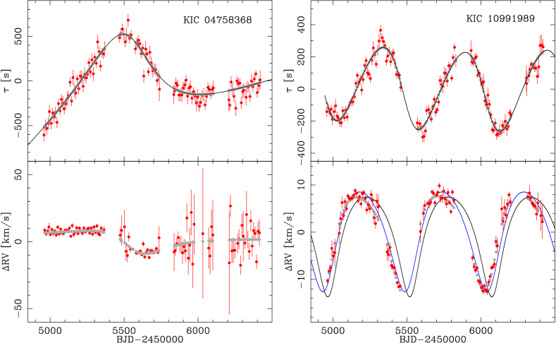
Figure 1: Illustration of the method of translating ETV measurements to RVs, on the ETV data for KIC 04758368 (left) and KIC10991989 (right). Top: Red points show our ETV measurements $\tau^{i}$, the black line is the generic fit to these data, and the grey dots are the model ETVs $\tau_{0}^{i}$. Bottom: Reproduced RVs of the centre of mass of the eclipsing binaries in these systems with scatter (red) and without (model, grey points). For KIC 10991989 solid lines present theoretical RV curves for a set of orbital parameters representing the best-fitting solution from Rappaport et al. (2013) (black), and for a set with values within their uncertainties (blue). The latter is in agreement with our reconstruction.

Calculating numerical derivative of a noisy sequence of data, like Kepler ’s ETVs, is quite challenging. Thus first we take our ETV measurements $\tau^{i}$ and fit a generic model ETV curve, that has no physical meaning, and is used only to get the shape of the timing variations and their probable “model” values $\tau_{0}^{i}$. This function can be periodic, but can also be a simple polynomial or spline (useful when ETVs do not cover the full orbital period). Having the “model” ETVs tabulated, it is fairly easy to calculate their derivatives and obtain the “model” radial velocity measurements. We do this with the simple two-point approach, for two consecutive ETVs $\tau_{0}^{i}$, $\tau_{0}^{i+1}$, measured in times $t^{i}$ and $t^{i+1}$:

$$v_{r,0}^{i}=c\frac{\tau_{0}^{i+1}-\tau_{0}^{i}}{t^{i+1}-t^{i}},$$ (9)

except for breaks between observations longer than 10 days. The time stamp is the mid-time of the two measurements, and $c$ is the speed of light. Now, we introduce the scatter to each of the model RVs. Intuitively, it is dependent on the difference between two measured ETVs. We define the correction to the $i$-th “model” RV $\epsilon_{v}^{i}$ = $v^{i}-v_{0}^{i}$ as the fraction of the measured and model ETV differences, multiplied by $c$ and the time-related term (as in the previous Equation):

$$\epsilon_{v}^{i}=c\frac{\tau^{i+1}-\tau^{i}}{\tau_{0}^{i+1}-\tau_{0}^{i}}\frac{1}{t^{i+1}-t^{i}}.$$ (10)

In this way we make the scatter of the RVs dependent on the scatter of the ETVs. We then tabulate the time stamps $(t^{i+1}+t^{i})/2$, scattered RVs $v_{r}^{i}=v_{r,0}^{i}+\epsilon_{v}^{i}$. We also calculate RV uncertainties $\sigma_{v}^{i}$, because in general each ETV can be given with a different error $\sigma_{\tau}^{i}$:

$$\sigma_{v}^{i}=c\frac{\sqrt{(\sigma_{\tau}^{i+1})^{2}+(\sigma_{\tau}^{i})^{2}}}{|\tau_{0}^{i+1}-\tau_{0}^{i}|}\frac{1}{t^{i+1}-t^{i}}.$$ (11)

Finally, we run two iterations of a sigma-clipping procedure to remove the obvious outliers. Their number does not exceed 10 per cent of all post-ETV radial velocities. The resulting RVs are given in Table 10, and our original ETVs in Table 11, both in the Appendix.

Our approach and its result is seen in the Figure 1. It works very well for periodic cases, like KIC 10991989, where ETVs cover several periods of the outer orbit. We can compare our reconstructed RVs to a model based on the solution from Rappaport et al. (2013), who give $P=554.2$ d, $e=0.30^{+0.07}_{-0.09}$, $A=256^{+18}_{-17}$ s, which leads to $K=10.56\pm 0.61$ km s^-1(ratio of two amplitudes: $K/A=0.041(4)$). One can see that our method gives RVs in agreement with this solution – in Fig. 1 the blue line represents a solution with parameters within the uncertainties given by Rappaport et al., and it passes through our post-ETV velocities. Analogous comparison can not be made for KIC 04758368, for which the solutions are highly uncertain due to a very long period, nor for KIC 05598639, for which no attempt to solve the ETVs have been made.

One can see that many post-ETV velocities of KIC 04758368 have large error and show a scatter comparable to or even larger than the RV amplitude itself (as seen from the model RVs), especially for BJD$>$2455800. This is actually expected when the scatter of ETVs is comparable to or larger than the scale of their variation. Radial velocities are time derivatives of the ETVs, so the more stable ETVs the less precise RVs. Our method also has the potential to verify the ephemeris of the inner eclipsing binary. Incorrect $P_{ecl}$ will lead to a linear trend in ETVs that may not be easily seen in some cases. In such case the post-ETV velocities will show a constant shift (non-zero $\gamma$), that may be easily detectable. A change in $P_{ecl}$ (meaning a non-zero $\dot{P}_{ecl}$), that may originate from a mass transfer for example, will produce a linear trend in RVs.

Note that our approach includes only the Römer time delay, not the longer time-scale perturbations, like the physical delay (Rappaport et al., 2013; Borkovits et al., 2015). Similar calculations can of course be done for timing of other periodic phenomena, like pulsations.

4.5 Orbital solutions

The orbital solutions were found with our own procedure called v2fit (Konacki et al., 2010). This code fits a single or double-keplerian orbit to a set of RV measurements of one or two components, utilizing the Levenberg-Marquard minimization scheme. The simplest version fits the period $P$, zero-phase $T_{0}$, systemic velocity $\gamma$, velocity semi-amplitudes $K_{1,2}$, eccentricity $e$ and periastron longitude $\omega$, although in the final runs the last two parameters were sometimes kept fixed on values found by jktebop fit (see next 4.6). The v2fit code allows for some perturbations and secondary effects, such us differences between zero-points of multiple spectrographs, or difference between systemic velocities of two components, $\Delta\gamma\equiv\gamma_{2}-\gamma_{1}$, which in this work was used for post-ETV RVs. The v2fit can also fit for linear and quadratic trends in $\gamma$, and periodic modulations of $\gamma$, interpreted as influence of a circumbinary body on an outer orbit. In the most sophisticated version it also employs the Wilson-Devinney (WD) code to account for tidal distortions of both components, as well as a number of relativistic effects, but these corrections were not used in this work, nor were the perturbations of $\gamma$. The code further calculates the projected values of major semi-axes $a_{1,2}\sin{i}$, and minimum masses $M_{1,2}\sin^{3}{i}$ for the SB2s. Whenever applicable, we simplified our fit by keeping the orbital period on the value given in the KEBC. Also, we were first letting $e$ and $\omega$ to be fit for, but when the resulting value of $e$ was indifferent from zero, we were keeping it fixed. Other parameters (when applicable) were always set free, unless clearly stated in the further text.

Formal parameter errors of the fit are estimated by forcing the final reduced $\chi^{2}$ to be close to 1, either by adding in quadrature a systematic term to the errors of RV measurements (jitter), or multiplying them by a certain factor. Because the code weights the measurements on the basis of their own errors, which are sensitive to $S/N$ and $v_{rot}$, we used the second option in our analysis. The errors given in Tables 8, 9, and 10 are the multiplied ones, for which $\chi^{2}\simeq 1$. Systematics coming from fixing a certain parameter in the fit are assessed by a Monte-Carlo procedure, and other possible systematics (like coming from poor sampling, low number of measurements, pulsations, etc.) by a bootstrap analysis. All the uncertainties of orbital parameters given in this work already include the systematics.

4.6 Light curve solutions

To deal with large amounts of photometric data from the Kepler telescope for multiple targets, one either needs a lot of computer time, or a fast, efficient, and somewhat simplified code. For the purpose of this work we choose the second option, and made sure that the simplifications either do not affect the final results or are properly taken into account in the error budget.

For the light curve (LC) analysis we used version 28 (v28) of the code jktebop (Southworth et al., 2004a, b), which is based on the ebop program (Popper & Etzel, 1981). It is a fast procedure that works on one set of photometric data at a time, and in the version we used, not allowing for analysis of RV curves. It also does not allow for spots or pulsations. It however offers a number of algorithms to properly include systematics in the error budget. The exquisite precision of Kepler photometry reveals all sort of out-of-eclipse brightness modulations in the DEBs, mainly spots and pulsations. In our objects, however, after years of nearly continuous observations they are averaged out over the orbital period. This results in a spread of data points in the phase-folded LCs that is larger than the telescope’s photometric precision (sometimes quite significantly). For this reason we decided to treat them as a correlated noise and run the residual-shifts (RS) procedure to calculate reliable uncertainties (Southworth et al., 2011). However, the time required to run the code in RS mode scales as the square of the number of data points.

Therefore, for finding the best fit we used the whole curve, but for the errors estimation we decided to analyse data from each quarter separately. Kepler’s long-cadence complete Q0-Q17 curves contain over 60,000 points, while single-quarter ones do not exceed 5000, so the time required to run the RS stage was at least 8 times shorter. For the systems with longest periods ($>$100 days) we sometimes merged two quarters into one set, in order to have both primary and secondary eclipse completely covered. We then calculated weighted averages of the resulting parameters. To get final parameter errors, we added in quadrature the formal error of the weighted average and the rms of the results from each quarter or set. When the additional variability was of a time scale much shorter than the length of a quarter (like oscillations), it made the weighted average error dominant. If the variability was of a longer time scale (like stable spots), it produced trends in parameters visible from quarter to quarter, and made the rms dominant. We believe that in such way we took care of the systematics in the LC analysis.

We fitted for the period $P$, mid-time of the primary (deeper) minimum $T_{ecl}$, sum of the fractional radii $r_{1}+r_{2}$ (where $r=R/a$), their ratio $k$, inclination $i$, surface brightness ratio $J$, maximum brightness $S$, and third light contribution $L_{3}$ for multiples. In case of eccentric SB1 systems, which can be recognized by the secondary eclipse located at a phase different than 0.5, we also fitted for $e$ and $\omega$, as the low number of spectroscopic data does not allow to constrain them securely. Their final values are from the jktebop runs. The gravity darkening coefficients were always kept fixed at the values appropriate for stars with convective envelopes ($g=0.32$). Due to the nature of studied objects, we did not use any spectroscopic ratios, which somewhat increased the resulting uncertainties in $k$. At the end, the code calculates the fractional radii $r_{1,2}$, and fluxes $L_{1,2}$.

4.7 Absolute parameters and age from isochrones

In case of those SB1 systems for which we performed the jktebop analysis, we can estimate the absolute stellar parameters and age of a system by comparing our partial results with theoretical isochrones. For this purpose we chose the PARSEC set (Bressan et al., 2012), which includes calculation of absolute magnitudes in the Kepler photometric band. We use the parameters from jktebop runs, i.e. $F=L_{2}/L_{1}$, $rr=r_{1}+r_{2}$, and $k=r_{2}/r_{1}$, and we look for such values of masses of the two stars and their age, that minimize the following term:

$$\chi^{2}=\left(\frac{k_{is}-k_{JK}}{\sigma_{k}}\right)^{2}+\left(\frac{rr_{is}-rr_{JK}}{\sigma_{rr}}\right)^{2}+\left(\frac{F_{is}-F_{JK}}{\sigma_{F}}\right)^{2},$$ (12)

where index $is$ denotes the values for a given pair of stars found in the isochrones, and parameters with the index $JK$ and the corresponding uncertainties $\sigma$ are taken from the jktebop solutions. For a set of ages, the PARSEC isochrones list masses, gravities, effective temperatures, and absolute magnitudes in the Kepler and SDSS bands. To calculate the fractional radii of the given pair of putative stars (to be compared with jktebop results), we first calculated the major semi-axis from our value of period and the putative masses, and then the radii using the masses and gravities. The Kepler band flux ratio $F=L_{2}/L_{1}$ was estimated from the difference of two putative absolute magnitudes. The search was performed for ages $t$ between $10^{6.6}$ and $10^{10.1}$ Gyr, with the step of 0.05 in $\log(t)$, with the additional condition that the secondary must be smaller, and either hotter or cooler than the primary, depending on the results of orbital fits. Sometimes we added an additional constrain regarding the SDSS $g^{\prime}-r^{\prime}$ colour. Finally, from the difference of observed and absolute magnitudes $kmag-Kmag$ for the whole system, and the primary alone if a total eclipse is observed, we can estimate the distance to the pair.

The analysis described here was performed only for one value of metallicity, which was taken from the MAST, and without any interpolation between nodes within a single isochrone, nor between isochrones. For this reason we did not attempt to estimate the uncertainties, and we treat the results as approximate, however self-consistent. The cited ages should be treated with caution, but the evolutionary stages should be determined securely.

5 Results

5.1 RV standards and stability

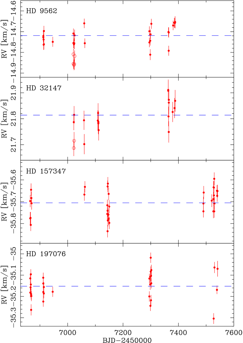
Figure 2: Results of RV measurements of the standards stars. Points taken for the analysis are marked with filled circles, while open symbols show values from December 2014 before the correction (for HD 9562 and HD 32147 only). Dashed lines mark the average values.

Table 2: Results for the radial velocity standards. For each star its spectral type, $V$-band magnitude, average RV ($\bar{v}$, in km s^-1), $rms$ (in km s^-1), number of measurements ($N$) and time span ($\Delta t$, in days) is given.

Star	Sp.T.	$V$	$\bar{v}$	$rms$	$N$	$\Delta t$
HD 9562	G1 V	5.76	-14.719	0.044	28	476
HD 32147	K3 V	6.21	21.814	0.054	19	366
HD 157347	G3 V	6.29	-35.705	0.060	36	676
HD 197076	G5 V	6.44	-35.152	0.064	30	676

The long-term stability of the spectrograph was monitored with observations and RV measurements of four radial velocity standards: HD 9562, HD 32147, HD 157347, and HD 197076. The first two were observed during the unfortunate run when the instrument set-up was changed, and allowed for the spectrograph’s zero-point correction. For this purpose for each of the two stars we calculated the average velocities during the unaffected observations, and shifted all measurements by that value. We then combined the two sets and for both stars calculated the shift of the December 2014 measurements only: $-0.100(10)$ km s^-1, and corrected them by this value. Finally, for both stars, we have calculated the average RVs and $rms$ again. Values of all velocities from the December run were then increased by 100 m s^-1.

The results of observations of standards are summarized in Table 2 and Figure 2. In case of the December 2014 run both corrected and uncorrected RVs are shown in the figure, but the final results from the table include only the corrected. We found the spectrograph to be stable to $\sim$40-60 m s^-1 over the course of our observations, and even down to 30 m s^-1 for shorter periods of 3-5 months. Some of the orbital solutions we found reach even lower $rms$, even below 20. Note that we were not using the iodine cell and not taking ThAr exposures before and after each science spectrum. For comparison, the precision achieved with HIDES with iodine cell is 5-20 m s^-1 (Sato et al., 2013a, b).

5.2 No orbital RV motion

In this section we present two objects where no orbital motion has been detected in the RVs. These are KIC 08718273 – a blend of a DEB with a foreground star, and KIC 05598639 – a confirmed visual binary that contains an eclipsing component, which is not detected in the spectra. We present strong clues that the latter system may, however, host additional, sub-stellar body.

5.2.1 KIC 08718273 – a blend with a foreground giant

This system has been observed nine times with HIDES by us, and twice by the APOGEE survey. We noted only one set of lines, whose measured velocity occurred to be relatively stable, with $rms=68$ m s^-1, which was slightly more than for the RV standards. Phase-folding with period from the KEBC of 6.959 d, or half of this value, and fitting a sine function, did not lead to any improvement. This confirmed the conclusions of Gaulme et al. (2013) that the oscillations they found are coming from a red giant not related to the eclipsing pair. We thus observe a blend. We perform a fit to the RVs in order to detected a signal that could be induced by the oscillations, but the details are described in Section 5.5. Due to a relatively large number of degrees of freedom, we used this fit to look for the difference between HIDES (plus ATLAS 9/12 templates) and APOGEE RV systems, which we found to be 112$\pm$22 m s^-1. We used it to shift APOGEE measurements of other targets, and included its uncertainty to the individual measurement errors. This case also confirms the correctness of the instrumental correction we found for the December 2014 run. Furthermore, we have found no trend indicating orbital motion around the centre of mass common with the eclipsing pair, confirming previous conclusions.

5.2.2 KIC 05598639 – a possible multiple

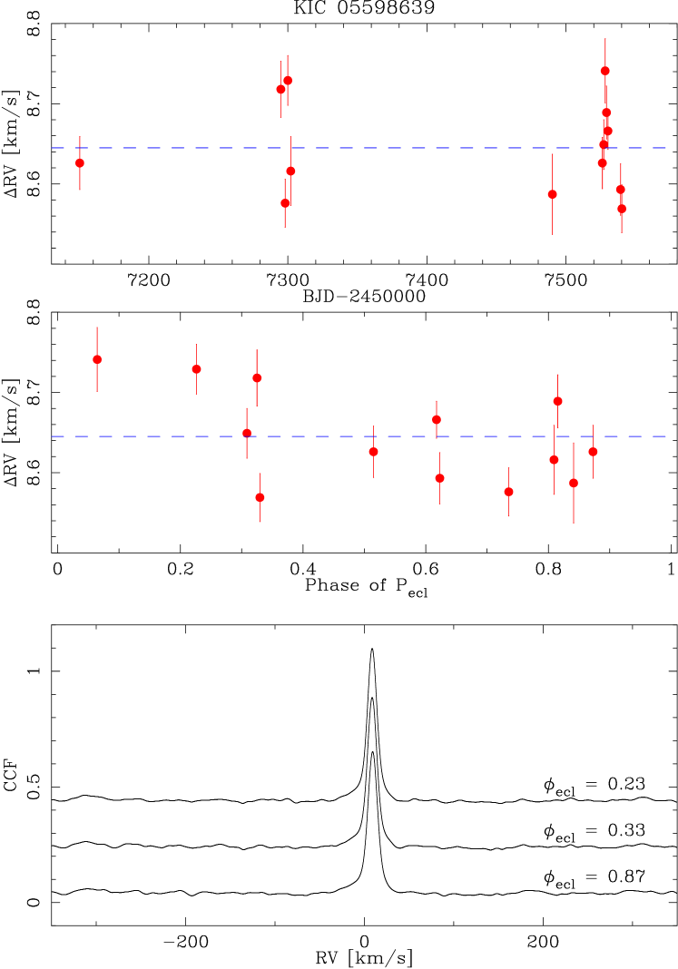
Figure 3: Top: Our HIDES radial velocities of KIC 05598639 as a function of time. The blue line marks the average measured velocity. The $rms$ is 59 m s^-1. Middle: Same, but phase-folded with the ephemeris of the eclipsing pair. No change related to the KEBC ephemeris is seen. Bottom: Three cross-correlation functions (CCFs), for spectra taken during different phases of the eclipsing binary $\phi_{ecl}$, shifted for clarity. Only one narrow peak is seen, and no others, that could be coming from the eclipsing binary, can be identified.

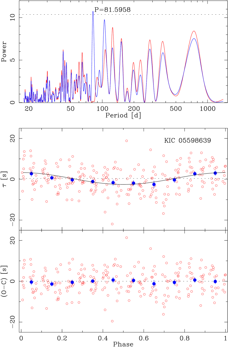
Figure 4: Top: Periodograms of our ETV measurements of KIC 05598639. The blue line is for the original data, for which the highest peak at 81.6 days is marked. The red line is for the data after this period is removed. The dotted line marks the FAP of 0.5%. Middle: Our ETV measurements phase-folded with the period of 81.6 days. Red points are original data, and blue points are data binned over 0.1 in orbital phase. The black solid line is the best cosine fit to the ETVs, and the dotted line is set at zero, for comparison. Bottom: Residuals of the best cosine fit to the ETVs.

To date we have obtained thirteen HIDES observations of this system, and were not able to find any other spectroscopic data. The light curve shows two wide, equal-depth eclipses and relatively strong ellipsoidal variations. Assuming that the eclipsing pair is composed of two solar-analogues, and taking $P_{ecl}=1.29755$ d from KEBC, we would expect to see two sets of equal lines, rotationally widened to $\sim$40 km s^-1  ($\propto R$), showing velocity variation with semi-amplitude of $>$120 km s^-1  ($\propto M^{1/3}$). Meanwhile, we only see one set of narrow lines, that is relatively stable (Fig. 3). The jktebop solution suggests that the eclipsing pair contributes only 38 per cent to the total flux, so the lines seen in the spectra probably come from the brighter component of the visual pair, and the fainter is the eclipsing binary observed by Kepler. The resulting magnitude difference – 0.53 mag – is not in agreement with the WDS value. The measured RVs are stable down to $\sim$60 m s^-1, which is the level of the $rm$ of RV standards. We therefore conclude that no significant motion can be detected in our data.

The ETVs calculated by Conroy et al. (2014) seem to be affected by strong systematics, so we have calculated our own, as in 4.3. We found no obvious periodicity at first, but we run a Lomb-Scargle periodogram on our measurements. We searched for periods between 18 and 1433 days (the time span $W$ of the data), using fixed frequency step of $1/10W=6.98\times 10^{-5}$ d^-1. The results are shown in Figure 4.

The highest peak of the periodogram was found at 81.6 days, but it was not much higher than the second one at 104.86 d. We fitted a cosine function with the 81.6 d period, and found the amplitude $A$ of $2.71\pm 0.56$ s (formal uncertainty of the fit only). This fit is also shown in Figure 4. To show the change of the ETVs with more clarity, we also plot data binned over 0.1 in phase. At the given period, the amplitude corresponds to minimum mass function of the outer body of $f(m)=3.21(66)\times 10^{-6}$ M_⊙, or $3.36(69)\times 10^{-3}$ M_JUP. Assuming that the total mass of the inner binary $M_{tot}$ is 2 M_⊙, and the outer body is significantly less massive than the eclipsing binary, its lower mass limit is then $m\sin(i)=25(1)$ M_JUP ($\propto M_{tot}^{2/3}$). We would like to note that $M_{tot}$ may actually be around 1 M_⊙, or less. Huber et al. (2014) estimated the mass of the dominant component (the one we see in spectra) to be $0.796^{+0.112}_{-0.073}$ M_⊙. The components of the inner binary should then be even less massive, possibly below 0.5 M_⊙ each. The $M_{tot}$ of 1 M_⊙ gives $m\sin(i)\sim 15$ M_JUP, pushing the outer body’s lower mass close to the planetary value. However, due to lack of direct information about the eclipsing pair, and large uncertainties of values from Huber et al. and our eclipse timing solutions, we find this possibility rather unlikely.

The eclipse timing amplitude we found is 2.2 times smaller than the $rms$ of the fit (6.018 s), thus we can not conclude that this periodicity is real, but is detected at 4.8$\sigma$ level ($\Delta A/A$), and we estimate the false-alarm probability to about 0.36 per cent. We also note that on the periodogram of the residuals (shown in Fig. 4 as the red line), the peak at 104.86 d is not the most prominent one. If the 81.6 d period of the eclipsing pair is real, the system may be a hierarchical quadruple, bearing a circumbinary brown dwarf, or even a massive planet. To confirm that, one needs more precise eclipse timing measurements and more spectroscopic observations. The true character of KIC 05598639 remains unknown, and more observations are planned.

5.3 RV motion not coinciding with $P_{ecl}$

In this section we present the analysis of two cases – KIC 04758368 and 10991989 – where the observed RV variations do not coincide with the period of eclipses seen in the Kepler data. They are hierarchical triple systems with the third (outer) star dominating the flux and seen in the spectra. They were treated as double-lined spectroscopic binaries, and parameters of their outer orbits were derived. The RVs of the centre of mass of the inner pair were obtained by translating the eclipse timing variations, as described in Section 4.4, but they contain limited information on the systemic velocity of the common centre of mass (CCM) $\gamma$. In order to find it, the inner pair was treated in the v2fit code as the primary and $\gamma_{1}$ was fitted for. The outer star (dominant in flux) was the secondary, and $\Delta\gamma$ has been found. The true systemic velocity of the CCM is thus $\Delta\gamma-\gamma_{1}$.

Although it may be the dominant source of flux in the triple, the outer star is always designated as the component B, and the inner eclipsing binary as A (Aa+Ab). The results are summarised in Table 3. As previously, uncertainties include systematics calculated with a bootstrap routine. Among other parameters, we show times of the pericentre passage $T_{per}$, number of data points for each component $N_{A,B}$ (note there are many more from ETVs than from direct RVs, but are much more spread), and the pericentre longitude given for the inner binary. We also give the systemic velocity of the whole triple as $\gamma$.

Moreover, for these two targets the jktebop fits were performed to estimate the contribution of each component to the total flux, inclination of the inner orbit, and fractional radii of the inner components – $R_{Aa}/a_{A}$ and $R_{Ab}/a_{A}$. Using the literature estimates of mass of the outer star $M_{B}$, we calculate the inclination of the outer orbit $i_{AB}$, total mass of the inner pair $M_{A}$, its major semi-axis $a_{A}$, and absolute radii $R_{Aa}$ and $R_{Ab}$.

Table 3: Orbital and stellar parameters of two hierarchical triples showing lines of the outer star in their spectra.

KIC	04758368	10991989
Outer orbit
$P_{AB}$ (d)	2553(80)	547.81(56)
$T_{0}$ (BJD-2450000)	5581(9)	5490(2)
$K_{A}$ (km s-1)	8.81(41)	10.28(13)
$K_{B}$ (km s-1)	12.9(1.4)	7.91(11)
$e_{AB}$	0.672(37)	0.251(7)
$\omega_{A}$ (∘)	141.9(2.1)	18.6(1.2)
$\gamma$ (km s-1)	-24.0(1.2)	-18.78(16)
$M_{A}\sin^{3}(i)$ (M⊙)	0.65(18)	0.135(4)
$M_{B}\sin^{3}(i)$ (M⊙)	0.45(9)	0.175(5)
$a_{AB}\sin(i)$ (AU)	3.77(32)	0.886(8)
$N_{A}$	106	101
$N_{B}$	19	14
$rms_{A}$ (km s-1)	6.9	1.22
$rms_{B}$ (m s-1)	57	25a
jktebop solution
$r_{Aa}+r_{Ab}$	0.4252(64)	0.373(10)
$r_{Ab}/r_{Aa}$	1.22(21)	0.657(58)
$L_{B}/L_{tot}$	0.725(19)	0.9764(54)
$i_{A}$ (∘)	73.94(79)	85.6(1.5)
Absolute values
$M_{B}$ (M⊙)	1.43 / 0.85${}_{-0.02}^{+0.43\,b}$	2.5(4)c
$i_{AB}$ (∘)	43 / 53.7${}_{-12.3}^{+5.7}$	24.3(1.4)
$M_{A}$ (M⊙)	2.1 / 1.24${}_{-0.15}^{+0.65}$	1.92(31)
$a_{AB}$ (AU)	5.3 / 4.68${}_{-0.67}^{+1.50}$	2.15(12)
$a_{A}$ (R⊙)	13.0 / 10.92${}_{-1.56}^{+3.50}$	5.14(28)
$R_{Aa}$ (R⊙)	2.48(30) / 2.09${}_{-0.39}^{+0.72}$	1.16(7)
$R_{Ab}$ (R⊙)	3.04(23) / 2.56${}_{-0.42}^{+0.84}$	0.81(6)

^aBefore fitting for the oscillations.
^bFrom the KIC (without errors) and Huber et al. (2014).
^cFrom Gaulme et al. (2013).

5.3.1 KIC 04758368

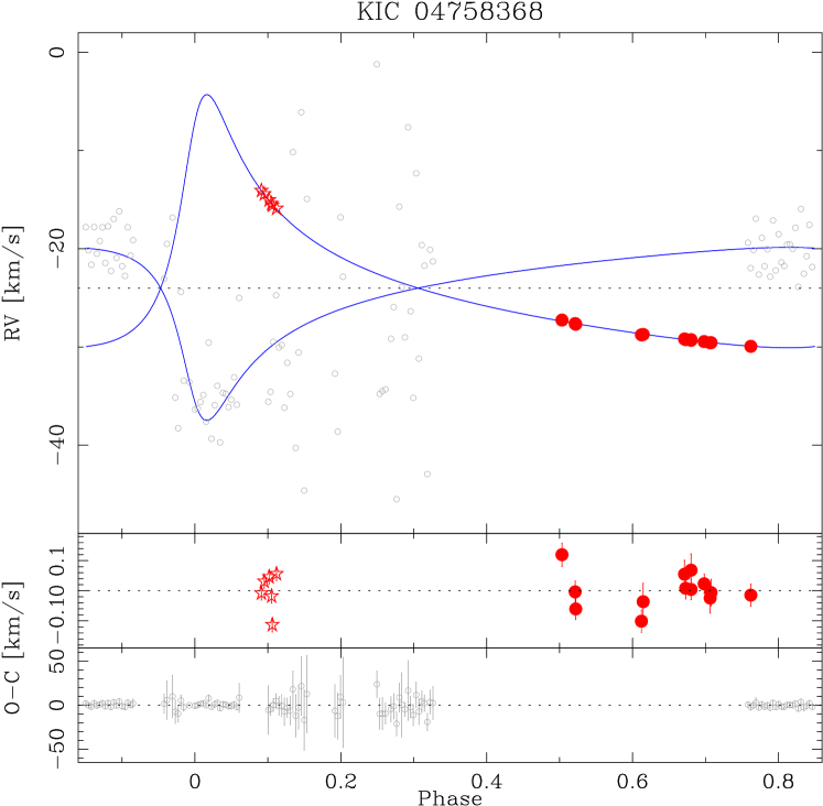
Figure 5: Orbital solution of the outer orbit of KIC 04758368. Grey points show the RVs of the centre of mass of the inner eclipsing binary, reconstructed from the ETV measurements, and shifted to the systemic velocity of the whole triple (dotted line). Red points are the direct RV measurements of the outer star, taken from the APOGEE data base (opens stars), and from our HIDES spectra (filled circles). Blue lines show the best-fitting orbital solution. Phase 0 is set to the moment of the pericentre passage. Lower panels show the residuals of the fit, separately for the direct and post-ETV measurements.

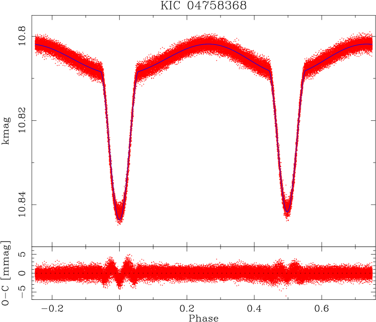
Figure 6: jktebop light curve solution for KIC 04758368.

The very long outer period of this system (the longest in the sample) makes it very difficult to analyse with the currently available data. The ETV measurements do not cover it completely, but their distinct maximum around JD$\sim$2455400, which means a sudden change in radial velocity, suggests that the inner binary passed the outer orbit’s pericentre that time (Fig. 1). Conroy et al. (2014) do not give the complete orbital solution, and the one by Borkovits et al. (2016) is marked as uncertain.

Our thirteen HIDES RV measurements cover even smaller fraction of the period, so the APOGEE data were very important. Initially, the post-ETV data were showing a best-fitting period of about 1600 days, which for the May 2015 (JD$\sim$2457150) observations predicted orbital phases roughly around the pericentre, i.e. RVs significantly higher than obtained from the previous HIDES runs. However, the measured velocity was still decreasing a year later – in May 2016 (JD$\sim$2457527), meaning that the star still did not pass the periastron, and that the period is actually longer than $\sim$2200 days. We still don’t have enough data to securely give its value, and we treat our solution as preliminary.

The best-fitting orbital model is shown in Figure 5, and corresponding parameters in Table 3. The main source of uncertainty is the orbital period, which may still be longer than we give, and its uncertainty underestimated. Another one are the errors and scatter of post-ETV velocities, mainly between phases 0.1 and 0.4, where the ETVs show a small curvature, comparable to or smaller than their scatter (Fig. 1).

We found that the third star is less massive than the inner binary, and constitutes about 72 per cent of the total flux. Gaulme et al. (2013) identify it as a non-oscillating red giant, and two estimates of mass/radius/gravity for this star can be found in catalogues. The MAST archive gives $\log(g_{B})=2.624\pm 0.400$ (from the KIC) and $R_{B}=9.651$ R_⊙ (without errors, from Christiansen et al., 2012), which translates into 1.43 $M_{\odot}$. Huber et al. (2014) give the revised $\log(g_{B})=2.610^{+0.261}_{-0.254}$, and estimates $R_{B}=7.55^{+3.49}_{-2.14}$ R_⊙ and $M_{B}=0.85^{+0.43}_{-0.02}$ M_⊙ ($\pm 68$ per cent confidence level).

In Table 3 we also show the absolute mass of the inner pair and parameters of the outer orbit, assuming the two values of $M_{B}$. We note that the Kepler light curve (Figure 6) shows nearly equal eclipses, suggesting nearly identical parameters of the components, and substantial ellipsoidal variations, suggesting their large size, relatively to their physical separation. The period of the inner orbit is 3.75 d, so we find it plausible that the components Aa and Ab are actually sub-giants, with masses comparable to or higher than the Sun, only significantly larger This is in agreement with the estimates of their absolute radii. All this favours the physical parameters of the star B found in the MAST archive, or around the upper limit of Huber’s values. The whole system would thus be relatively old, which agrees with the metal abundance estimate [$M/H$]=-0.46 dex (from both KIC and Huber et al., 2014). However, as it will be discussed later in this work, the MAST values of $\log(g)$ may be overestimated.

We would also like to note that in this case the APOGEE archive gives very different values of $log(g)$ and [$M/H$] of 2.24(11) and 0.01(3) dex, respectively. It is possibly because the analysis was done on an averaged spectrum, made of six visit spectra, each having different heliocentric velocity. Averaging such spectra, without a prior velocity correction, might have resulted in a spectrum with lines wider than they really are.

5.3.2 KIC 10991989

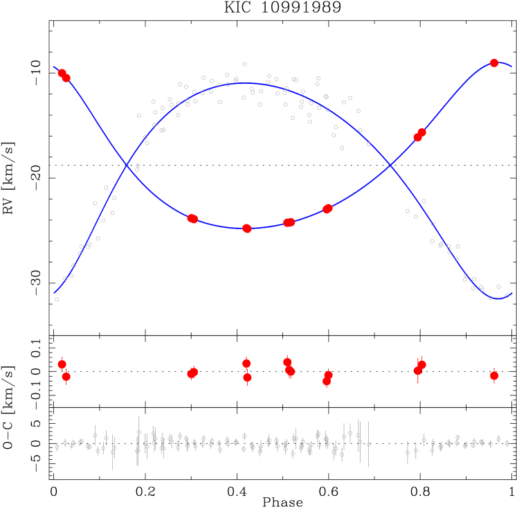
Figure 7: Same as Fig. 5, but for KIC 10991989. All directly measured RVs (red points) come from our HIDES spectra.

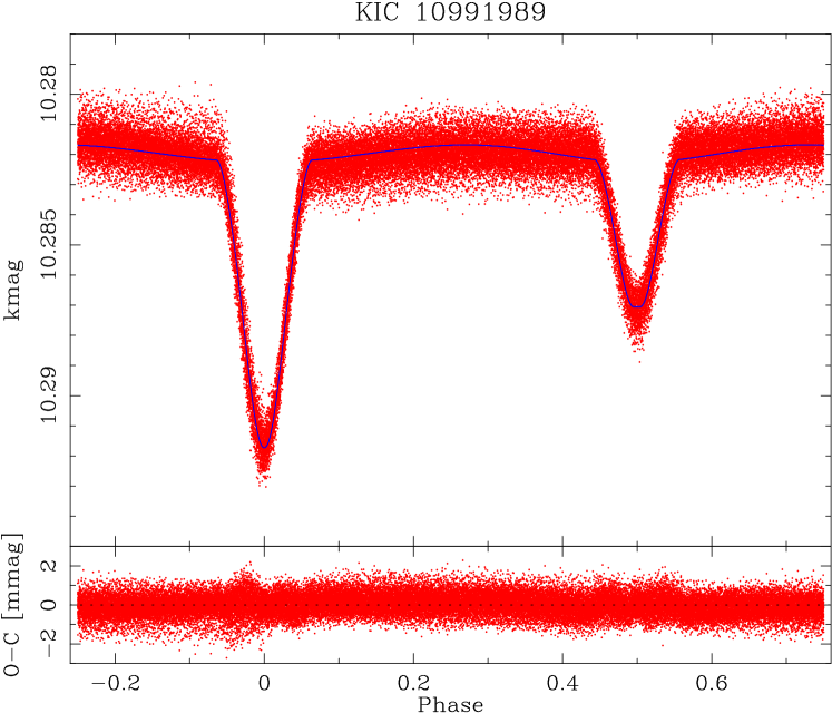
Figure 8: Same as Fig. 6, but for KIC 10991989.

We have observed this system fourteen times with HIDES, covering the period of the outer orbit almost completely, and the ETVs cover almost 2.5 cycles (Fig. 1). Our solution is depicted in Figure 7 with parameters summarized in Table 3. Our results for the outer orbit agree with those of Rappaport et al. (2013) in terms of orbital parameters, i.e. $e_{AB},\omega_{A},M_{A,B}\sin^{3}(i)$, and the mass ratio $M_{B}/(M_{A}+M_{B})$, however their uncertainties are quite large. A slight disagreement is seen in ephemeris – $P_{AB}$=547.81(56) vs. 554.2 d, and $T_{per}=2455490(2)$ vs. $2455525.7^{+21}_{-18}$ – although Rappaport et al. do not give the uncertainty of their outer period. The outer period in the solution of Borkovits et al. (2016) is in a much better agreement with ours – 548(1) d – but their $e$ and $\omega$ are not, being 0.35(2) and 29(4)^∘, respectively. We find another solution, by Conroy et al. (2014), less reliable, because it assumes a circular orbit, while our direct RVs show a substantial eccentricity.

We also used the component B (pulsating red giant) mass estimate from Gaulme et al. (2013), and calculated the total mass of the inner binary, and outer orbit’s inclination. By combining this with the results from jktebop run (Figure 8), we can estimate the inner orbit’s major semi-axis, and absolute radii of Aa and Ab. The results are also shown in Table 3. Additionally, we estimate (from the jktebop analysis) that the outer star contributes 97.6 per cent to the total flux. The inner binary is composed of two stars of significantly different radii (note that the secondary eclipse is total), and different spectral types (as can be deduced from unequal eclipses, for example). Considering the resulted radii $R_{Aa}$ and $R_{Ab}$, it’s possible that the inner pair is composed of $\sim$1.15+0.75 M_⊙ main sequence stars. At least one component shows a substantial level of activity – single-quarter Kepler light curves reveal out-of-eclipse modulation coming from cold spots that slowly evolve in time. The fact that the brightness of the system in both minima varies with the same scale, suggests similar influence of spots on the flux of both stars. This means that the secondary, which is likely much smaller and cooler than the primary, must have relatively larger area covered in spots.

5.4 RV motion coinciding with $P_{ecl}$

In this section we present results for five single-lined spectroscopic binaries (SB1), i.e. systems for which the period of the RVs is the same as of the eclipses. With the exception of KIC 10614012, these systems show both eclipses in the Kepler data. For those we performed a jktebop analysis to find the inclination, fractional radii, brightness ratio, as well as period, eccentricity and longitude of pericentre. Last three parameters were used in v2fit, with which we found the systemic velocity, velocity amplitude, moment of the periastron passage or quadrature (for $e=0$), and the major semi-axis of the primary’s orbit around the centre of mass. These results are summarised in Table 4.

Further comparison with isochrones was also made to estimate the absolute values of stellar parameters, age, and distance. These results are shown in Table 5.

Table 4: v2fit and jktebop solutions for KIC 03120320, 08430105, 10001167, and 10015516.

Parameter	03210320	08430105	10001167	10015516
$P$ (d)	10.2656136(4)	63.32717(5)	120.39110(26)	67.692165(15)
$T_{0}$ (BJD-2450000)a	4956.29(26)	4985.91(42)	5064.0(1.1)	5022.291(8)
$T_{ecl}$ (BJD-2450000)b	4959.22316(3)	4976.6345(7)	4957.6827(19)	5005.38019(18)
$e$	0.034(5)	0.256(72)	0.160(2)	0.0(fix)
$\omega$ (∘)	343(9)	350.5(1.6)	213(1)	—
$K_{1}$ (km s-1)	39.23(9)	27.66(13)	24.9(7)	32.162(54)
$\gamma$ (km s-1)	-41.10(26)	11.5(1.0)	-103.2(1.1)	-16.471(37)
$a_{1}\sin(i)$ (AU)	0.03700(24)	0.1556(8)	0.272(8)	0.20012(34)
$a_{1}\sin(i)$ (R⊙)	7.956(2)	33.47(16)	58.5(1.7)	43.03(7)
$f(M_{2})$ (M⊙)	0.06411(44)	0.1254(74)	0.185(16)	0.2333(12)
$r_{1}$	0.05898(44)	0.0893(21)	0.112(18)	0.0982(1)
$r_{2}$	0.02287(65)	0.00905(37)	0.0085(20)	0.01536(20)
$i$ (∘)	87.845(73)	88.53(53)	86.6(1.9)	86.85(10)
$L_{2}/L_{1}$	0.0127(7)	0.01729(46)	0.0189(9)	0.1046(20)
$rms_{RV}$ (m s-1)	153	71	137	34
$rms_{LC}$ (mmag)	0.92	0.66	1.3	0.69

^a Time of periastron passage ($e>0$) or quadrature ($e=0$).
^b Mid-time of primary (deeper) eclipse.

Table 5: Results of the isochrone mass/age search for KIC 03120320, 08430105, 10001167, and 10015516.

Parameter	03120320		0843105		10001167		10015516
	jktebop	Isochrones	jktebop	Isochrones	jktebop	Isochrones	jktebop	Isochrones
$r_{1}+r_{2}$	0.08186(66)	0.08178	0.0985(35)	0.01021	0.121(19)	0.122	0.1136(10)	0.1128
$r_{2}/r_{1}$	0.388(9)	0.4122	0.1006(25)	0.1016	0.0764(65)	0.0757	0.1563(22)	0.1564
$L_{2}/L_{1}$	0.0127(7)	0.0123	0.01729(46)	0.01716	0.0189(9)	0.0190	0.1046(20)	0.1038
Individual, absolute
	Primary	Secondary	Primary	Secondary	Primary	Secondary	Primary	Secondary
$M$ (M⊙)	1.019	0.550	1.042	0.790	1.135	0.993	2.024	1.480
$R$ (R⊙)	1.338	0.552	7.582	0.770	14.984	1.134	10.363	1.620
$\log(g)$	3.926	4.696	2.576	4.562	2.084	4.326	2.577	4.189
$T_{eff}$ (K)	5780	3945	4890	5790	4750	6430	4960	7610
$Kmag$ (mag)	3.430	8.204	0.905	5.319	-0.269	4.034	0.081	2.527
$K$ (km s-1)a	39.23	73.1	27.7	33.47	24.9	28.4	32.16	42.39
Whole system
$\left[M/H\right]^{b}$	-0.24		-0.60		-0.50		-0.22
$t$ (Gyr)	7.94		6.31		4.47		1.26
$d$ (kpc)c	0.31		0.81		1.17		1.40

^aDirectly from Tab. 4 for the primary. ^bFrom MAST. ^cAssuming no interstellar extinction.

5.4.1 KIC 03120320

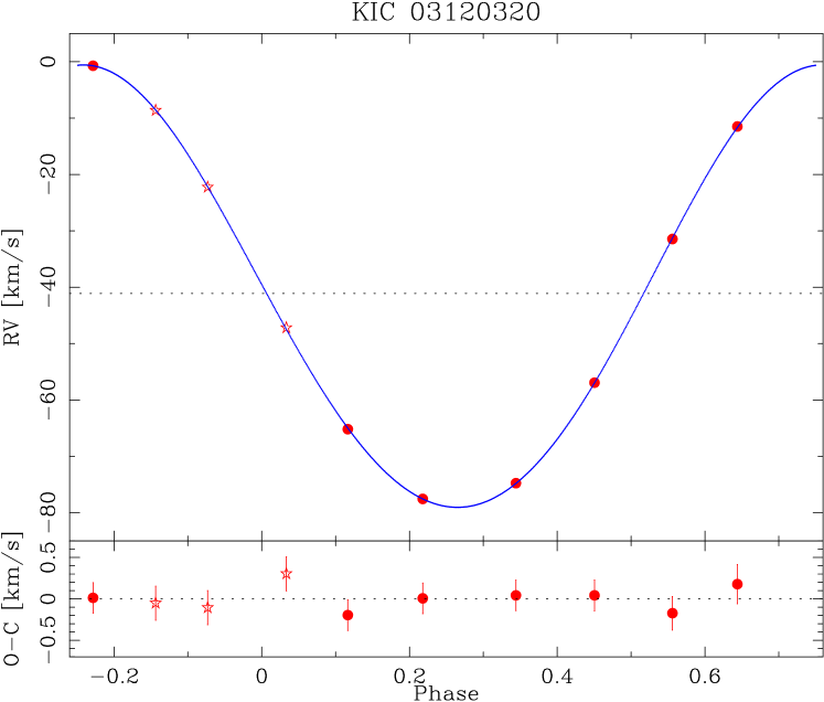
Figure 9: Left: Orbital fit (blue line) to our HIDES (filled circles) and APOGEE (open stars) RVs of KIC 03120320, phase-folded with the ephemeris from Table 4 ($P,T_{ecl}$). The decrease of the velocity during phase 0 (deeper eclipse) means that the RVs are measured for the hotter component. Right jktebop fit the the complete Q0-Q17 curve.

This target has been observed seven times with HIDES by us, and three more by the APOGEE survey. Among the four SB1s analysed with jktebop this is the only one where the primary eclipse is not total, and the component visible in the spectra is the hotter one. This can be deduced from the fact that its RV decreases during the primary eclipse. The secondary one is not at the phase 0.5, meaning that the orbit is slightly elliptical. Also, the fit to the RVs is slightly better for a non-circular orbit, than for $e=0$. Results of our fits are summarised in Table 4, and on Figure 9. We note an out-of-eclipse modulation, most likely coming from the presence of spots on the primary. Its influence on the RV measurements may explain the relatively large $rms$ of the orbital fit.

On the [$M/H$]=-0.24 dex PARSEC isochrone, we found a good match to jktebop values for a $1.019+0.550$ M_⊙ pair at the age of almost 8 Gyr ($\log(t)=9.90$). The primary is somewhat evolved, with the radius of $1.338$ R_⊙, and entered the sub-giant phase, while the secondary is on the main sequence ($R_{2}=0.552$ R_⊙). Its lines should be detectable on very high $S/N$ ratio spectra, especially in infra-red. The secondary should be highly active, and its emission lines may be seen. Unfortunately, HIDES does not reach to the calcium H and K lines, where such emission would be easiest to note. Assuming no interstellar extinction, we estimate the distance to this pair to 311 pc, thus it should be measurable by the Gaia satellite.

We would like to note that even better match was found for a $0.932+0.517$ M_⊙ pair at the age of 11.2 Gyr ($\log(t)=10.05$). However, we found this solution less reliable, as the predicted $g^{\prime}-r^{\prime}$ colour is 0.554 mag, which is significantly redder than the observed 0.453. The solution we adopted predicts $g^{\prime}-r^{\prime}=0.440$ mag, and the difference can be attributed to the reddening, or uncertainties of jktebop results or the metallicity. It is worse in terms of $\chi^{2}$ mainly due to the disagreement in ratio of the radii $k$. This is because, when both eclipses are partial, this parameter is not constrained very well by the light curve only. The usual way of solving this issue is by using spectroscopy-based flux ratios. This is, however, impossible when lines of the secondary are not visible in the spectra. We suspect that our uncertainties in $k$ (and $L_{2}/L_{1}$) for this system may be underestimated, but still the agreement with the isochrone values is better than 3$\sigma$.

5.4.2 KIC 08430105

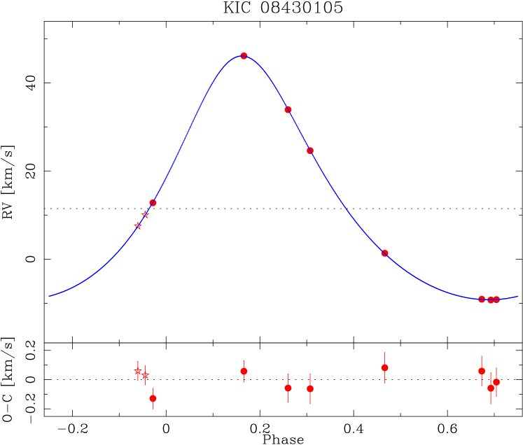
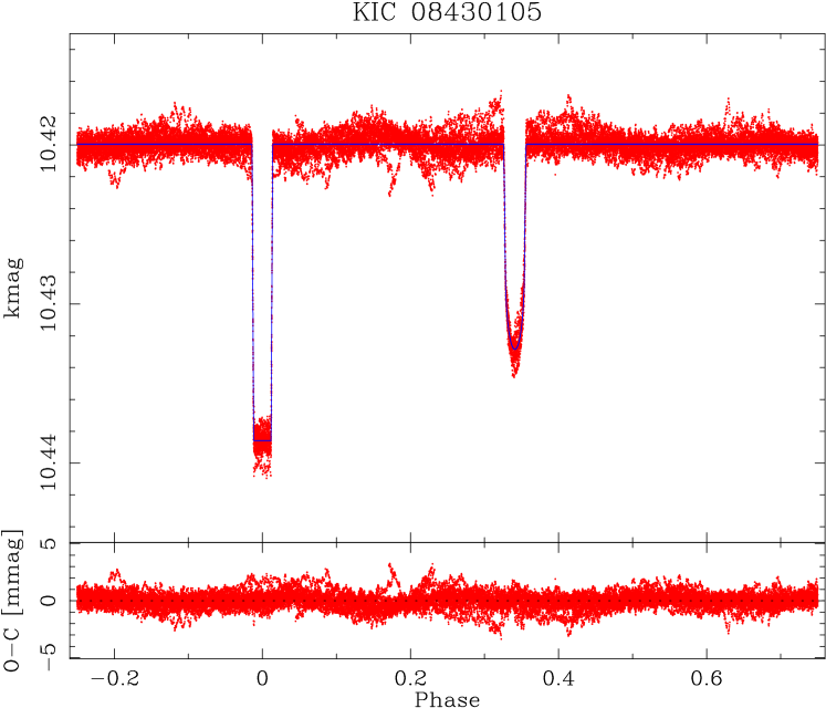
Figure 10: Same as Fig. 9 but for KIC 08430105. The increase of the velocity (left) during phase 0 (deeper eclipse) means that the RVs are measured for the cooler component.

It is the first of three SB1 systems in our sample that show a total primary eclipse, which helps a lot in the LC analysis. It is also the most metal-poor among them, with [$M/H$]=-0.596 dex (from MAST). We have acquired eight spectra with HIDES, and found two more observations in the APOGEE archive. The data points are spread more-less evenly throughout the orbital period, including phases around maximum and minimum of the RV curve therefore the RV-based parameters – $T_{per},K_{1}$, and $\gamma$ – are constrained quite well. The final $rms=71$ m s^-1  is comparable to those of the RV standards. Also, $e$ and $\omega$ can be estimated precisely from the light curve. Results of our fits are summarised in Table 4, and on Figure 10.

From the fact that the RV curve rises during the total primary eclipse, we can deduce that the primary is cooler and larger than the secondary. Indeed, comparison with the PARSEC isochrone for [$M/H$]=-0.596 shows that the best match is found for a $1.042+0.790$ M_⊙ pair at the age of 6.3 Gyr ($\log(t)=9.80$). The primary is a red giant ($R_{1}=7.582$ R_⊙), and its parameters, especially the mass, are in agreement with the results from asteroseismologic analysis of Gaulme et al. (2014): $M_{1}=1.04(12)$ M_⊙ and $R_{1}=7.14(28)$ R_⊙. The secondary is still a main-sequence ($R_{2}=0.770$ R_⊙), late G- or early K-type star. It’s lines should be detectable on very high $S/N$ spectra. With such a long period, this could be an interesting target for testing the influence of rotation and activity on observed radii and temperatures of lower-main-sequence stars. But a direct measurements of its RVs are required.

From the difference of observed and absolute magnitudes $kmag-Kmag$, under the assumption of negligible extinction, we estimate the distance to the pair to be 807 pc. In this case the the extinction is probably not negligible, so the true distance is larger.

5.4.3 KIC 10001167

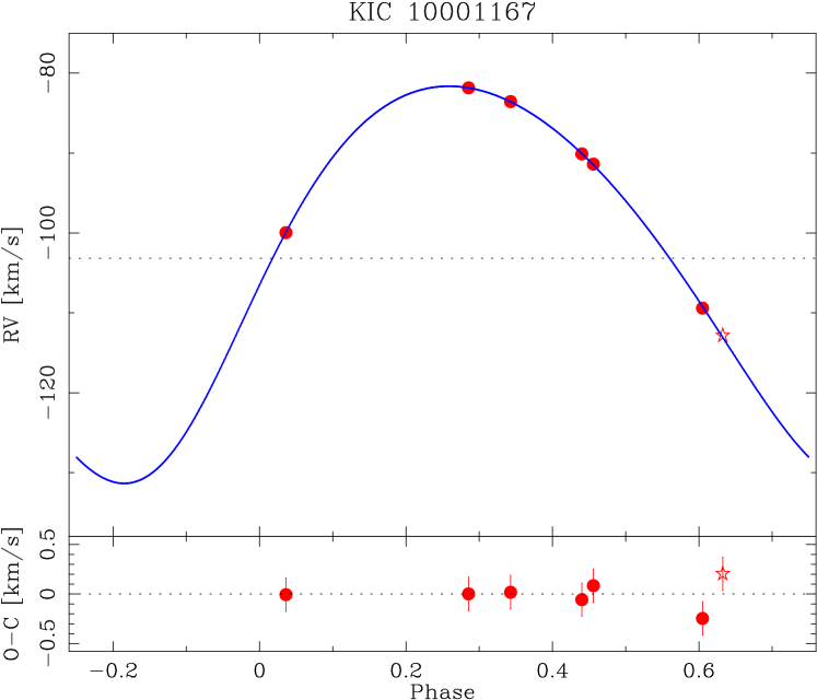
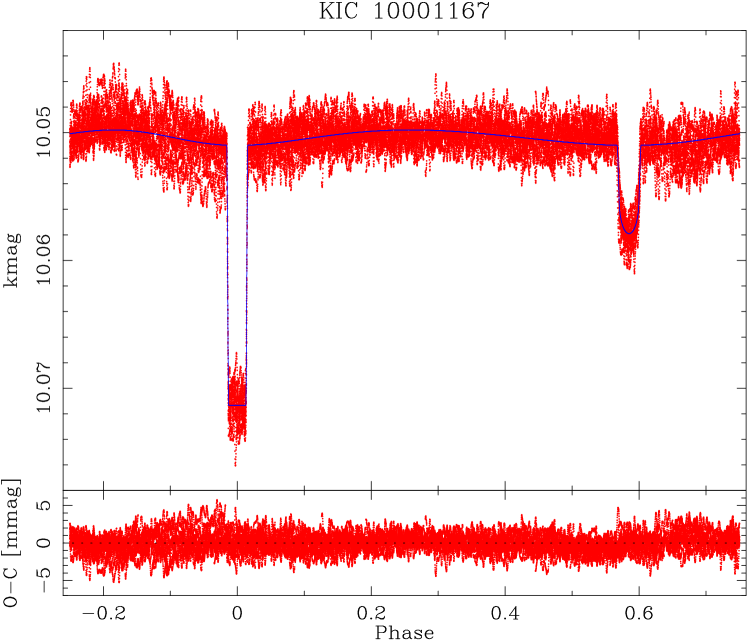
Figure 11: Same as Fig. 9 but for KIC 10001167. The increase of the velocity (left) during phase 0 (deeper eclipse) means that the RVs are measured for the cooler component.

This system has one APOGEE and six HIDES data points, which is the lowest number of data points on our sample. This, and the fact that the phases where velocity is the lowest, are not properly covered, are the main reasons of high uncertainties in the RV-based parameters. The target also shows additional variability of the largest-scale ($rms_{LC}=1.3$ mmag), therefore the LC-based parameters dependent on the depths of eclipses (like $i$ or $r_{1,2}$) are the least precise. As in the previous case, the behaviour of the RV curve around the primary eclipse suggests that the star visible in the spectra is the cooler and larger one. The results are shown in Table 4, and on Figure 11.

The comparison with PARSEC isochrone for [$M/H$]=$-0.504$ dex showed that this pair is likely composed of a 1.135 M_⊙ red giant ($R_{1}=14.984$ R_⊙), currently during an early phase of burning helium in its core, and a 0.993 M_⊙ main sequence star ($R_{2}=1.134$ R_⊙). The best-fitting age is 4.47 Gyr ($\log(t)=9.65$). Due to large errors in $rr,k$ and $F$, these results are however uncertain. The distance estimated from the difference of observed and absolute Kepler magnitudes, assuming no extinction, is 1.17 kpc. It does not agree with 705 pc estimated by Gontcharov (2008). He estimated the extinction to be 0.24 mag in $V$, which is similar to 0.29 mag, which can be derived from the MAST entry ($E(B-V)$=0.094; assuming $R=3.1$). Even taking 0.29 mag as the value of extinction in the Kepler bandpass, (which should be lower than in $V$ because of the longer wavelength) it is not enough to explain this discrepancy.

We found two other very good matches: for a $1.70+1.15$ M_⊙ pair at the age of 1.6 Gyr ($\log(t)=9.2$), and for a $4.80+2.69$ M_⊙ pair at the age of 0.1 Gyr ($\log(t)=8.0$). The latter solution predicted $g^{\prime}-r^{\prime}=0.142$ mag, which is much bluer than the observed 0.831, and would require very strong reddening. The $1.70+1.15$ M_⊙ scenario, and the one we adopted ($1.135+0.993$ M_⊙), predict $g^{\prime}-r^{\prime}=0.746$ and 0.752 mag, respectively. Our preferred solution is in much better agreement with the asteroseismic parameters of the giant from Gaulme et al. (2014), which are $M_{1}=1.13(7)$ M_⊙ and $R_{1}=13.85(32)$ R_⊙. Notably, as for KIC 0843105, the mass of the primary that we found from isochrones, matches the asteroseismologic results much better than the radius. For the record, the $1.70+1.15$ M_⊙ scenario gives radii of 15.93 and 1.20 R_⊙.

In any case, the primary of KIC 10001167 is the largest star in our sample. The fact that it is in the core helium burning phase is interesting by itself. KIC 10001167 seems to be a valuable target for further studies. Better understanding of this system would be possible if secondary’s velocities were directly measured, and multi-band photometry obtained, especially in the total primary eclipse. This would give direct measurement of both stars’ masses, radii and effective temperatures. Sufficient photometry is not that challenging, whereas the spectroscopy would require high $S/N$ observations in the blue ($<$5000 Å).

5.4.4 KIC 10015516

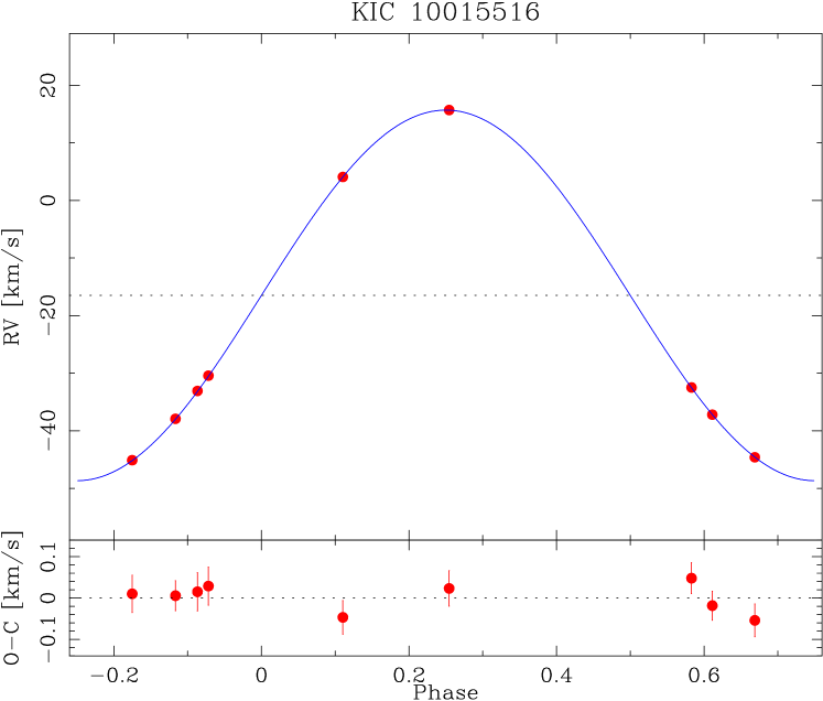
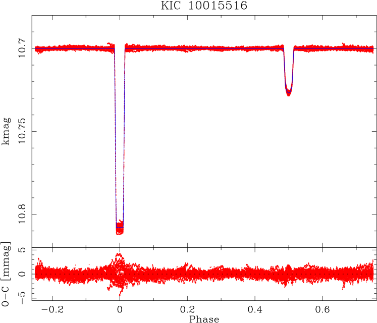
Figure 12: Same as Fig. 9 but for KIC 10015516 and our HIDES data only in the RV panel (left). The increase of the velocity during phase 0 (deeper eclipse) means that the RVs are measured for the cooler component.

We observed this system nine times with HIDES; no APOGEE or other publicly available spectra were found. Also in this case, the component visible in the spectra is the cooler one, and the primary eclipse is total. In the jktebop fit we found the orbit indifferent from circular, thus, to simplify our v2fit run and the RS stage of jktebop, we set $e$ to 0.0 and held fixed. Despite the largest number of degrees of freedom, we reached a very good $rms$ of the RVs of only 34 m s^-1. The results are presented in Table 4 and in Figure 12.

This system has the largest mass function $f$ among the four SB1s with jktebop models. It is also the only one with circular orbit, despite a relatively long period. We thus suspected that both stars are fairly massive, the colder one being much more evolved than in previous cases, and the hotter, probably of type A, still residing at the main sequence. The best fitting PARSEC isochrone of [$M/H$]=-0.22 dex was found for the age of 1.26 Gyr ($\log(t)=9.1$), and the preferred masses are 2.024 and 1.480 M_⊙ for the primary and secondary, respectively, which makes KIC 10015516 the most massive system in our sample. The estimated distance of 1.4 kpc is also the largest from all systems described in this section. The best-fitting isochrone predicts the secondary to be an A8, main sequence star ($R_{2}=1.620$ R_⊙). The primary is found to be a red giant ($R_{1}=10.363$ R_⊙) during a late stage of core helium burning, just before moving to the asymptotic giant branch. Such configuration is a relatively unusual one for a DEB, so KIC 10015516, together with the previous target, seems to be an valuable target for studies of very late stages of stellar evolution. Again, better understanding of this system would come with direct measurements of secondary’s RVs (presumably from observations in $\lambda<5000$ Å), and multi-band photometry.

5.4.5 KIC 10614012 – “heartbeat” SB1

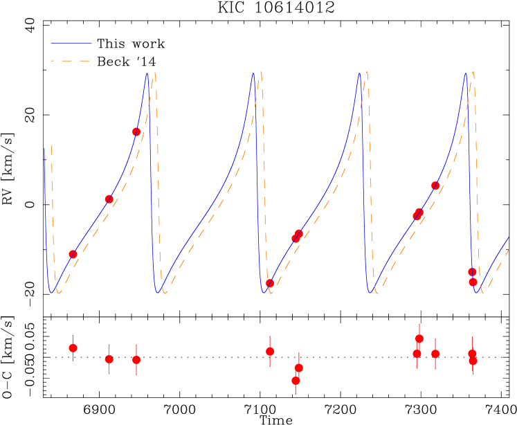
Figure 13: Our HIDES RV measurements (red points) of KIC 10614012 as a function of time, together with two different solutions: from this work (blue solid line) and the exact solution from Beck et al. (2014, orange dashed). The lower panel shows residuals of our solution.

Table 6: Our orbital solution of KIC 10614012 and comparison with the one by Beck et al. (2014).

Parameter	This work	Beck ’14
$P$ (d)	132.132(1)	132.13(1)
$T_{per}$ (BJD-2450000)	4981.38(6)	4990.48(1)
$e$	0.709(4)	0.71(1)
$\omega$ (∘)	71.5(4)	70.5(5)
$K_{1}$ (km s-1)	24.46(28)	24.68(3)
$\gamma$ (km s-1)	-0.67(5)	-0.92(2)
$a_{1}\sin(i)$ (AU)	0.209(3)	0.211(3)
$f(M_{2})$ (M⊙)	0.070(2)	0.072(3)
$rms$ (m s-1)	26	—
$M_{2}$ (M⊙)a	0.67(24)	0.68(24)
$K_{2}$ (km s-1)	51(34)	50(34)

^a Assuming $\sin^{3}(i)\simeq 1$ and $M_{1}=1.4(8)$ M_⊙.

This is an exception among our SB1s because we did not perform the jktebop analysis for this system. This is because jktebop is not able to model the brightness modulation around but outside the primary eclipse, and that there is no secondary eclipse in the light curve. With HIDES we have obtained eleven spectra of this SB1, and we are able to compare them with the orbital solution given by Beck et al. (2014) on the basis of their 22 Hermes spectra. We found immediately that their exact values of orbital parameters do not reproduce our measurements. We first examined the Kepler light curve and found that the periods given in KEBC (132.1673 d) and by Beck et al.. (132.13 d) are both not optimal, and we found a better one – 132.132(1) d – similar to the one from Beck et al., but more precise. We performed a new fit to our RVs, fitting all parameters but the period (i.e.: $T_{per},e,\omega,K_{1},\gamma$), and found a satisfactory solution with $rms$ of only 26 m s^-1. It is shown in Figure 13, with resulting parameters compared in Table 6.

Our new solution is quite similar to the one by Beck et al., but due to the lower number of our data, and poor coverage of the phases when the velocity is highest and around the pericentre passage, our estimate of the velocity amplitude is worse. The differences in systemic velocities and times of pericentre may be explained by different zero-points of HIDES (+ATLAS 9/12) and Hermes, and the slightly different values of orbital periods. The marginal agreement in $\omega$ may also suggest apsidal motion, which would also explain the difference in $T_{per}$. We can conclude that our measurements are in general agreement with Beck et al. (2014), but provide better constrains to the system’s ephemeris.

The object itself very interesting and unusual, as it is a member of a peculiar class of variables, called “heartbeat stars” (HBs), which are objects where pulsations were tidally induced by a companion, passing closely through the pericentre. Due to the eclipsing nature, KIC 10614012 is unusual even among the HBs. Using the obtained values of the mass function $f(m)$, the estimate of the mass of the (pulsating) primary from Beck et al. (2014) – 1.4(8) M_⊙ – and assuming $\sin^{3}(i)\simeq 1$ (from the existence of eclipses), we can estimate the mass of the secondary star $M_{2}=0.67(24)$ M_⊙, and the amplitude of its RV variation $K_{2}=51(34)$ km s^-1. These estimates are also given in Tab. 6 for each of the solutions. The depth of the eclipse itself is about 0.76 per cent in flux, which corresponds to the ratio of radii $k=\sqrt{0.0076}\simeq 0.087$, assuming negligible contribution of the secondary to the total flux. If the primary’s radius is 8.6(2) R_⊙ (Beck et al., 2014), then the secondary should have $\sim$0.75 R_⊙. It is in rough agreement with a 0.67 M_⊙ main sequence star if the large uncertainty is taken into account. Main sequence stars of this radius found in eclipsing binaries tend to have masses $>0.7$ M_⊙ (Southworth, 2015). KIC 10614012 is thus probably a pair composed of a red giant and a K dwarf.

5.5 RV signature of solar-like oscillations in giants

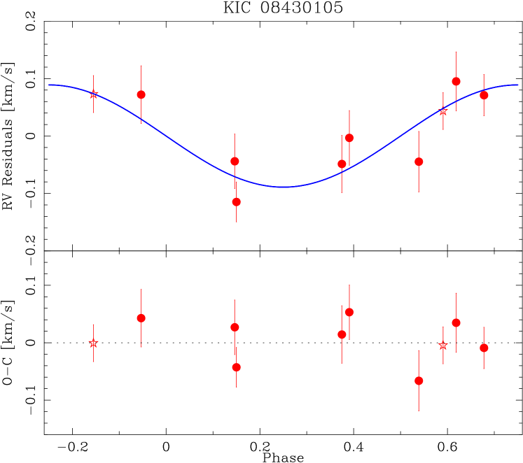
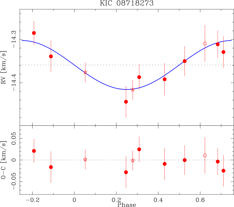
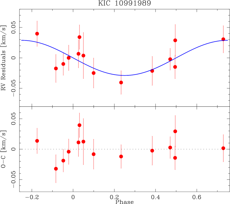
Figure 14: Our HIDES (circles) and APOGEE data (stars) for three of four oscillating red giants, phase folded with periods very close to the frequency of maximum amplitude. The blue lines represent sine functions fitted to the data, with parameters shown in Table 7. For KIC 08718273 (middle) we show direct RV measurements, and the open circle represents the measurement from the December 2014 run, shifted up by 100 m s^-1(see Sect. 5.1), matching the solution very well. For KIC 08430105 (top) and KIC 10991989 (bottom) we show residuals of the orbital fits, which were described earlier. The residuals of oscillation fits (lower panels) are shown in the same scale, for comparison.

Table 7: Results of the search for RV signals induced by oscillations.

	$\nu_{max}$	$P_{osc}$	$P^{\prime}_{osc}$	$K_{osc}$	$rms$	Det. level
KIC No.	($\mu$Hz)	(d)	(d)	(m s-1)	(m s-1)	($\sigma$)
08430105	66.80(1.64)	0.1733(43)	0.17310(2)	89(19)	71/38	4.60
08718273	28.30	0.409	0.40827(3)	57(8)	68/17	7.12
10991989	89.90	0.129	0.12875(5)	29(11)	25/19	2.64

Notes: The “$rms$” column shows the $rms$ before and after the fit to oscillations.
Uncertainty of $\nu_{max}$ was given in Gaulme et al. (2014), but not in Gaulme et al. (2013).

Four of the targets described in this work are known to show solar-like oscillations (Gaulme et al., 2013, 2014). Such oscillations not only contribute to the light curve of a system, but may also be affecting RVs, by introducing an additional scatter, and possibly mimic a presence of an additional body on a short-period orbit. We thus decided to look for their signature in our and APOGEE data.

For this we used the v2fit code, and assumed that the modulation is sinusoidal (i.e. mimicking a circular orbit). We took the frequencies of maximum amplitude ($\nu_{max}$), and translated into periods. We used these values as starting points for the period fit. In both cases we fitted for the amplitude $K_{osc}$, base velocity (which corresponds to the systemic velocity $\gamma$ in KIC 08718273, and in the other was indistinguishable from zero), and time of the zero phase (which has no significant physical meaning here).

The results are shown in Table 7 and Figure 14. In the Table we give values of $\nu_{max}$ and its corresponding period $P_{osc}$ (with errors, if available in the source), the period we found ($P^{\prime}_{osc}$), and the amplitude of the RV modulation ($K_{osc}$). We also compare the $rms$’s before and after the fit, and give the level of detection in $\sigma$ defined as $K_{osc}/\Delta K_{osc}$.

The signal is clearest in the case of KIC 0871273, reaching the level of over 7$\sigma$. The $rms$ of the 11 data points drops significantly after the fit, and the relative error of $K_{osc}$ is small. The second best case – KIC 08430105 – also showed a significant improvement after the fit, but the detection level is lower (4.60$\sigma$). The last case – KIC 10991989 – has he highest numbers of measurements, but the potential amplitude is the lowest. Detection at the level of 2.64$\sigma$ is only marginal. For the remaining system – KIC 10001167 – we can only say, that the behaviour of the residuals, and large $rms$ of the orbital fit may suggest the existence of an oscillation-induced RV signal, but we did not find any solution that could lower the $rms$ significantly. The number of data points is, however, still too small for a secure conclusion, therefore more observations are planned in the future.

We’d like to point out that the $rms$ before the fit for oscillations was already quite low in each case, and comparable to (for KIC 0840105 and 08718273) or better than (KIC 10991989) for the RV standards. The fit lowered the $rms$ below 40 m s^-1  (lowest $rms$ of a standard star) in each case, and it might be a coincidence that the periodicities we found in the data are very close to those expected from oscillations. Therefore we advise the readers to treat this result with caution.

6 Summary

We presented analysis of radial velocities, light curves, and eclipse timing variations of nine objects, found by the Kepler satellite to be eclipsing binaries. In all cases only one set of lines has been found in the spectra. In our sample we identified five single-lined binaries, two hierarchical triples, one possible quadruple with a circumbinary brown dwarf, and one blend. Using the theoretical stellar evolutionary models, we managed to estimate the absolute parameters of four SB1s. For the two hierarchical systems – KIC 04758368 and 10991989 – we translated the ETVs into RVs and derived parameters of the outer orbits, together with some of the physical properties of the inner binaries. These objects may prove to be valuable for models of multiple stellar systems formation.

The target selection criteria, mainly the limits for brightness and temperature, caused that many of our targets (6 out of 9) contain red giants, four of which were reported to be oscillating. In our spectroscopy we were able to detect RV signals with periods coinciding with the oscillation frequency $\nu_{max}$. For two of the giants – primary components of SB1s – the isochrone-based parameters are in a good agreement with asteroseismic results, which suggests the correctness of our approach. However, notably, the parameters derived from spectroscopy, and listed in the MAST archive, are not in agreement with ours. In particular, the MAST values of $\log(g)$ tend to be 0.25-0.50 dex higher than ours, found for four cases (see Table 5). Other quantities, such as [$M/H$], may, therefore, also be incorrect. We thus recommend to treat the MAST values with bigger caution.

From the point of view of stellar astrophysics, the objects we described show interesting properties. The components of each SB1 are clearly on very different evolutionary stages, sometimes very rarely observed in eclipsing binaries, like the core helium burning phase. Unfortunately, lines of the secondaries were not visible in our data. However, for some of them, i.e. those showing a total primary eclipse (KIC 0843105, 10001167 and 10015516), important information can be derived from observations in the totality (Hełminiak et al., 2015a). Further spectroscopic and photometric follow-up during the eclipse would be very useful.

Appendix A Radial velocities

In this Section we list the RV measurements used in our work. We group them in different tables, depending on their source and character. Longer tables are available in their full extent in the on-line version of the manuscript.

In Table 8 we show the RV measurements extracted from the APOGEE survey. This Table is complete. For the reference, each row contains the Plate ID, MJD, and fibre number – quantities useful to identify the observation in the survey’s website.

Our HIDES measurements of the nine systems described in this work are given in Table 9. This table includes exposure times, final errors, and approximate $S/N$ at 6000Å. Only a portion is shown here.

The Table 10 shows the post-ETV radial velocities, calculated for KIC 04758368 and 10991989. Again, only a portion is shown here, and the complete Table is available on-line.

Table 8: A complete set of APOGEE radial velocities used in this study. The last column is the identifier that can be used to find single visit spectra in the archive.

BJD	$v$	$\epsilon$	KIC	Plate ID-MJD-Fiber
-2450000	(km s-1)	(km s-1)
5811.612390	-47.200	0.177	03120320	5213-55811-254
5840.592682	-8.638	0.166	03120320	5213-55840-176
5851.579964	-22.274	0.144	03120320	5213-55851-152
5813.699707	-14.087	0.023	04758368	5214-55813-190
5823.726497	-14.439	0.023	04758368	5215-55823-196
5840.661140	-15.046	0.023	04758368	5215-55840-196
5849.578359	-15.419	0.023	04758368	5214-55849-196
5851.648750	-15.584	0.023	04758368	5215-55851-291
5866.569442	-15.902	0.022	04758368	5214-55866-159
6366.011412	7.517	0.038	08430105	6090-56365-034
6367.005991	10.042	0.036	08430105	6090-56366-034
6465.952143	-14.376	0.022	08718237	7018-56465-166
6470.943842	-14.416	0.022	08718237	7018-56470-154
5876.564815	-112.834	0.202	10001157	5552-55876-232

Table 9: HIDES radial velocities. Complete Table is available in the on-line version of the manuscript.

BJD	$v$	$\epsilon$	KIC	$t_{exp}$	$S/N$
-2450000	(km s-1)	(km s-1)		(s)
7300.979626	-65.177	0.186	03120320	1200	53
7302.021194	-77.543	0.185	03120320	1500	57
7317.970408	-0.718	0.185	03120320	1500	42
7490.272271	-31.445	0.203	03120320	1200	25
7491.174252	-11.494	0.237	03120320	1200	18
…
6866.045030	-27.260	0.039	04758368	1800	25
6912.149187	-27.616	0.036	04758368	1500	61
6914.194285	-27.683	0.035	04758368	1500	41
…

Table 10: Post-ETV radial velocities of centre of mass for two hierarchical triples. Complete Table is available in the on-line version of the manuscript.

BJD	$v$	$\epsilon$	KIC
-2450000	(km s-1)	(km s-1)
4963.618272	8.51	2.97	04758368
4973.452402	5.92	3.67	04758368
4982.969772	7.77	3.34	04758368
4991.623760	10.96	5.54	04758368
5001.473103	5.26	2.04	04758368
…
4963.617665	-10.33	0.66	10991989
4973.451707	-8.22	0.77	10991989
4982.969009	-7.56	0.84	10991989
4991.622949	-3.42	2.44	10991989
5001.472255	-5.06	1.47	10991989
…

Appendix B Eclipse timing variations

In the Table 11 we show our own measurements of eclipse timing variations for three system, as derived with the method described in Section 4.3.

Table 11: The eclipse timing variations used in this work ($\tau$) and their uncertainties $\epsilon$, calculated with the method of Kozłowski et al. (2011). Only a portion of the table is shown here, and the complete one is available on-line.

BJD	$\tau$	$\epsilon$	KIC
-2450000	(s)	(s)
4958.402347	-606	68	04758368
4968.834197	-494	61	04758368
4978.070606	-532	65	04758368
4987.868936	-476	64	04758368
…
4955.950945	-0.15	5.88	05598637
4960.742821	9.53	5.82	05598637
4965.534690	11.16	7.38	05598637
4970.326551	5.31	5.30	05598637
…
4958.401792	-141	31	10991989
4968.833539	-118	23	10991989
4978.069874	-147	20	10991989
4987.868143	-126	24	10991989
…

References

- Allende Prieto et al. (2008) Allende Prieto C. et al., 2008, Astr. Nachr., 329, 1018
- Beck et al. (2014) Beck P. G. et al., 2014, A&A, 564, A36
- Borkovits et al. (2015) Borkovits T., Rappaport S., Hajdu T., Sztakovics J., 2015, MNRAS, 448, 946
- Borkovits et al. (2016) Borkovits T., Hajdu T., Sztakovics J., Rappaport S., Levine A., Bíro I. B., 2016, MNRAS, 455, 4136
- Bressan et al. (2012) Bressan A., Marigo P., Girardi L., Salasnich B., Dal Cero C., Rubele S., Nanni A., 2012, MNRAS, 427, 127
- Christiansen et al. (2012) Christiansen J. L. et al. 2012, PASP, 124, 1279
- Conroy et al. (2014) Conroy K. E., Prša A., Stassun K. G., Orosz J. A. Fabrycky D. C., Welsh W. F., 2014, AJ, 147, 45
- Coughlin et al. (2011) Coughlin J. L., Lopez-Morales M., Harrison T. E., Ule N., Hoffman D. I., 2011, AJ, 141, 78
- Gies et al. (2012) Gies D. R., Williams S. J., Matson R. A., Guo Z., Thomas S. M., Orosz J. A., Peters G. J., 2012, AJ, 143, 137
- Gies et al. (2015) Gies D. R., Matson R. A., Guo Z., Lester K. V., Orosz J. A., Peters G. J., 2015, AJ, 150, 178
- Gaulme et al. (2013) Gaulme P., McKeever J., Rawls M. L., Jackiewicz J., Mosser B., Guzik J. A., 2013, ApJ, 767, 82
- Gaulme et al. (2014) Gaulme P., Jackiewicz J., Apporchaux T., Mosser B., 2014, ApJ, 785, 5
- Gontcharov (2008) Gontcharov, G. A. 2008, Astronomy Letters, 34, 785
- Heintz (1980) Heintz, W. D. 1980, ApJS, 44, 111
- Hełminiak et al. (2012) Hełminiak K. G. et al., 2012, MNRAS, 425, 1245
- Hełminiak et al. (2015a) Hełminiak K. G. et al., 2015a, MNRAS, 448, 1945
- Hełminiak et al. (2015b) Hełminiak K. G., Ukita N., Kambe E., Konacki M., 2015b, ApJL, 813, 25
- Huber et al. (2014) Huber D. et al., 2014, ApJS, 211, 2
- Izumiura (1999) Izumiura H., 1999, in: Proc. 4th East Asian Meeting on Astronomy, ed. P. S. Chen, Kunming, Yunnan Observatory, p. 77
- Kambe et al. (2013) Kambe E., et al., 2013, PASJ, 65, 15
- Kirk et al. (2016) Kirk B. et al., 2016, AJ, 151, 68
- Konacki et al. (2010) Konacki M., Muterspaugh M. W., Kulkarni S. R., Hełminiak, K. G., 2010, ApJ, 719, 1293
- Kozłowski et al. (2011) Kozłowski S. K., Konacki M., Sybilski P., 2011, MNRAS, 416, 2020
- Kurucz (1992) Kurucz R. L., 1992, in Barbury B., Renzini A., eds, Proc. IAU Symp. 149, The Stellar Population of Galaxies, Kluwer Academic Publishers, Dordrecht, p. 225
- Majewski et al. (2015) Majewski S. R. et al., 2015, preprint (arXiv:1509.05420)
- Mason et al. (2001) Mason B. D., Wycoff G. L., Hartkopf W. I., Douglass G. G., Worley, C. E., 2001, AJ, 122, 3466
- Matijevič et al. (2012) Matijevič G., Prša A., Orosz J. A., Welsh W. F., Bloemen S., Barclay T., 2012, AJ, 143, 123
- Popper & Etzel (1981) Popper D. M., Etzel P. B., 1981, AJ, 86, 102
- Prša et al. (2011) Prša A. et al., 2011, AJ, 141, 83
- Rappaport et al. (2013) Rappaport S., Deck K., Levine A., Borkovits T., Carter J., El Mellach I., Sanchis-Ojeda R., Kalomeni B., 2014, ApJ, 768, 33
- Santerne et al. (2016) Santerne A., 2016, A&A, 587, A64
- Sato et al. (2013a) Sato B. et al., 2013a, ApJ, 762, 9
- Sato et al. (2013b) Sato B. et al., 2013a, PASJ, 65, 85
- Slawson et al. (2011) Slawson R. W. et al., 2011, AJ, 142, 160
- Southworth (2015) Southworth J., 2015, ASPC, 496, 164
- Southworth et al. (2004a) Southworth J., Maxted P. F. L., Smalley B., 2004a, MNRAS, 351, 1277
- Southworth et al. (2004b) Southworth J., Zucker S., Maxted P. F. L., Smalley B., 2004b, MNRAS, 355, 986
- Southworth et al. (2011) Southworth J., Pavlovski K., Tamajo E., Smalley B., West R. G., Anderson D. R., 2011, MNRAS, 414, 3740
- Tenenbaum et al. (2012) Tenenbaum P. et al., 2012, ApJS, 199, 24