Three-Dimensional Orientation of Compact High Velocity Clouds

Abstract

We present a proof-of-concept study of a method to estimate the inclination angle of compact high velocity clouds (CHVCs), i.e. the angle between a CHVC’s trajectory and the line-of-sight. The inclination angle is derived from the CHVC’s morphology and kinematics. We calibrate the method with numerical simulations, and we apply it to a sample of CHVCs drawn from HIPASS. Implications for CHVC distances are discussed.

1 Motivation

The Galactic halo hosts a population of neutral hydrogen clouds whose line-of-sight velocities are inconsistent with Galactic rotation (Wakker & van Woerden, 1997). These High Velocity Clouds (HVCs) range from large “complexes” of many degrees to structures at the resolution limit. Their diversity suggests different origins (Wakker & van Woerden, 1997; Putman et al., 2012). Distances to HVCs are key to the origin question. The most accurate constraints stem from absorption line studies (Wakker, 2001; Wakker et al., 2007; Thom et al., 2006; Thom et al., 2008; Richter et al., 2015), yet these are only available for structures of large angular extent, and therefore are biased to near objects. Indirect distances via H$\alpha$ emission use the UV flux escaping from the disk and ionizing the HVCs (Putman et al., 2003). Uncertainties arise from determining the escape fraction of ionizing UV photons, though the patchiness of the disk interstellar gas ceases to be of concern for $|z|>10$ kpc (Bland-Hawthorn & Putman, 2001; Peek et al., 2007). Olano (2008) uses a putative origin to constrain distances of CHVCs spatially associated with the Magellanic complexes (also Peek et al., 2008; Saul et al., 2012). Distance constraints based on cloud kinematics assume a terminal velocity for HVCs (Benjamin & Danly, 1997) or rely on differential drag due to the interaction with the background medium (Peek et al., 2007). Both of these methods require the inclination angle between the cloud’s trajectory and the line-of-sight. Full trajectory information has been inferred in only a few cases (Smith Cloud: Lockman et al., 2008; Fox et al., 2016; Complex GCN: Jin, 2010).

We will focus our attention on compact high velocity clouds (CHVCs), many of whom show a head-tail structure, consisting of a cold, dense core, and a more diffuse, warmer tail (Brüns et al., 2000; Brüns et al., 2001). This morphology suggests that CHVCs interact with the ambient medium during their passage through the Galactic halo (Brüns et al., 2000; Stanimirović et al., 2006; Peek et al., 2007; Putman et al., 2011). Because of their small angular extent, distance estimates to CHVCs stem mostly from assumed association with larger complexes (Peek et al., 2008; Putman et al., 2011). Yet, an independent method is desirable. Because of their interaction with the ambient gas, CHVCs could in principle be used to gain information about the elusive gaseous component of the Galactic halo (Peek et al., 2007).

Instead of aiming directly at getting distances to CHVCs, we propose a method to determine the three-dimensional orientation of CHVCs and thus their full, three-dimensional velocity $\mathbf{v}_{tot}$. Consequences for distance constraints are discussed in Sec. 4.1.

2 The Method

The coordinate system is set by the local $(GL,GB)$ patch describing the plane-of-sky, and by the (unknown) cloud distance $D$ along the line-of-sight (Fig. 1). The three-dimensional orientation of a CHVC requires two angles: The inclination angle $0\leq\alpha_{i}\leq\pi$ describes the angle between the cloud tail and the line-of-sight, with the tail pointing away from the observer for $\alpha_{i}=0$. The position angle $0\leq\alpha_{p}<2\pi$ is counted counter-clockwise starting with $\alpha_{p}=0$ for the cloud’s tail pointing toward Galactic North. The local coordinate patch is assumed to be rectangular – hence the limitation to CHVCs.

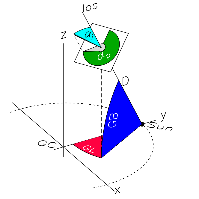
Figure 1: Definition of the coordinate system for CHVC orientation. The position angle $\alpha_{p}$ (green) and the inclination angle $\alpha_{i}$ (cyan) are defined in the local (GL,GB) patch, at an (unknown) distance $D$ from the Sun. A cartoon CHVC mapped within the local (GL,GB) patch is outlined in grey.

The goal is to relate the cloud shape in position-velocity space to the inclination angle. We demonstrate the process with the help of a simulation (Fig. 2) of a CHVC traveling at $\alpha_{i}=45^{\circ}$ toward the observer. The simulation (model Wb1a15b of Heitsch & Putman (2009), see their table 1 and fig. 2) is a wind-tunnel experiment, in which an initially spherical cloud of (in this case) radius $50$ pc and density $0.1$ cm^-3 is exposed to a wind of $150$ km s^-1 and a density of $10^{-5}$ cm^-3. The simulation generated $\sim 30$ 3D data sets consisting of gas density, velocity and temperature. These are converted into position-position-velocity cubes by selecting for gas with a temperature of $T<10^{4}$ K (assumed to be neutral hydrogen), rotating by the desired inclination angle $\alpha_{i0}$, and then calculating channel maps with $\Delta v=1$ km s^-1 assuming optically thin HI-21 cm emission. Peak column densities reach $\sim 3\times 10^{19}$ cm^-2. These channel maps are then used for further analysis.

The position angle $\alpha_{p}$ is determined by fitting ellipses to the integrated intensity maps. Since the orientation of the ellipse is degenerate with $\pi$, we identify the tail of the cloud as the direction in which the cloud extends farthest from the column density peak (i.e. the location of the head). This assumes that the clouds have a head-tail structure. To estimate the inclination angle, we define the cloud’s ”backbone” (i.e. the line through the cloud’s center-of-mass at the determined $\alpha_{p}$), along which spectra are taken to construct a position-velocity map (Fig. 2e-g). For a CHVC moving toward the observer, the (dense) core will appear at more negative velocities and the tail at more positive ones, hence the CHVC will be asymmetric along the velocity axis. Yet, along the position axis, the CHVC will appear more or less symmetric (Fig. 2d). If the CHVC moves perpendicularly to the line-of-sight, head and tail can be clearly identified, resulting in an asymmetry in position. Yet, the CHVC will appear symmetric in velocity space, since the gradient along the cloud backbone due to the differential drag will not be discernible, and only thermal and turbulent motions within the CHVC will contribute to the velocity signature (Fig. 2f). A CHVC traveling at e.g. $45^{\circ}$ to the observer will appear asymmetric both in position and velocity (Fig. 2e).

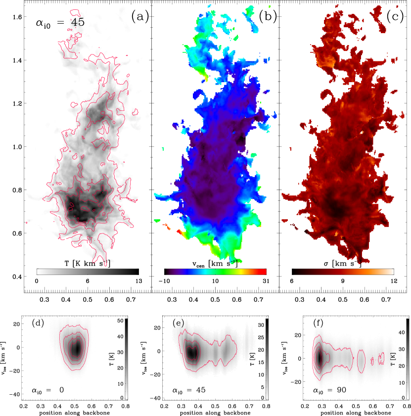
Figure 2: (a) Integrated intensity, (b) centroid velocity, and (c) velocity dispersion of a model CHVC (model Wb1a15b of Heitsch & Putman (2009)), traveling at $45^{\circ}$ to the observer. Contours are given at $[1,5,9,13]$ K km s^-1. (d,e,f) Position-velocity plots for inclination angles $\alpha_{i0}=0,45,90^{\circ}$. Contours correspond to $[5,15,25,35]$ K.

We calculate the observable asymmetry of the CHVC’s gas distribution with respect to its center-of-mass. The asymmetry in position is given by

$$a_{p}\equiv\frac{\Delta_{2p}-\Delta_{1p}}{\Delta_{1p}+\Delta_{2p}},$$ (1)

with $-1\leq a_{p}\leq 1$. The one-sided dispersions $\Delta_{1p,2p}$ refer to the CHVC extent to lower/higher values in position with respect to the center-of-mass, e.g.

$$\Delta_{1p}=\left(\sum_{p<p_{c},v}(p-p_{c})^{2}\,T(p,v)\bigg{/}\sum_{p<p_{c},v}T(p,v)\right)^{1/2},$$ (2)

where $T(p,v)$ is the position-velocity map, $p_{c}$ is the center-of-mass position, and the summation extends over all $p<p_{c}$ (along the horizontal axis in Fig. 2d-f), and over the whole velocity range. For $\Delta_{2p}$, the summation extends over $p>p_{c}$. The velocity extents $\Delta_{1v,2v}$ are constructed similarly, along the vertical (velocity) axis of the position-velocity plot. Other measures of cloud extent, such as $50$% contours, give similar results. Since the accuracy of $\Delta_{1,2}$ depends on the map resolution, spatial and velocity resolution of the telescope will affect the result. A CHVC with the tail pointing toward positive $p$ has $a_{p}>0$, and a CHVC moving toward the observer (tail toward positive $v$) has $a_{v}>0$. Since the asymmetries are normalized, and if we assume (to first order) a linear relationship between the velocity and the position along the cloud’s tail (see e.g. Brüns et al., 2001), we can calculate the inclination angle as

$$\alpha_{i}=\arctan\left(\frac{a_{p}}{a_{v}}\right).$$ (3)

To test the method, position-position-velocity cubes are generated for the CHVC model of Fig. 2, for a series of rotation angles $\alpha_{i0}$. ”Spectra” (position-velocity plots) are taken along the long axis of the cloud (Fig. 2d-f), from which we derive the inclination angle estimate $\alpha_{i}$. Fig. 3 summarizes the reliability of the inclination angle estimates. Panels (a) and (b) show $\alpha_{i}$ as derived from equation 3, and its residuals $\alpha_{i}-\alpha_{i0}$. Apart from occasional large deviations due to substantial fractions of gas being stripped off the CHVC, the residuals depend systematically on the model rotation angle $\alpha_{i0}$ (Fig. 3f). Therefore, we attempt to improve on equation 3 by fitting a heuristic function to the residuals; we average over the cloud evolution time (Fig. 3g, the error bars are errors on the mean). The resulting corrected values are shown in red in Fig. 3e through 3g, and Fig. 3b,d. The fitting function is given by

$$f(\alpha_{i0})=p_{0}\,\tanh\frac{\alpha_{i0}-p_{2}}{p_{3}}\,\exp\frac{\alpha_{i0}-p_{2}}{p_{4}}+p_{1}.$$ (4)

Parameter distributions and values derived from the Metropolis-Hastings algorithm used to fit equation 4 are given in the right column of Fig. 3.

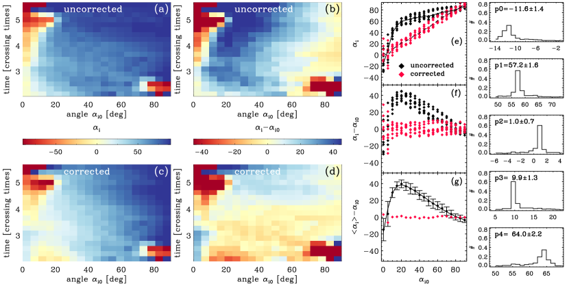
Figure 3: (a) Colour map of the uncorrected inclination angle estimate (equation 3) depending on the rotation angle $\alpha_{i0}$, and on the model CHVC evolution time. Large “secular” differences occur when substantial fragments are stripped off the CHVC. (b) Uncorrected inclination angle residuals scaled between $\pm 45^{\circ}$. (c) Corrected inclination angle estimates, and (d) corrected residuals. (e) Uncorrected (black) and corrected (red) inclination angles, and (f) their residuals. (g) Residuals calculated from averaged uncorrected inclination angle (black), empirical fit (line, see equation 4), and resulting corrected residuals (red). The right column gives the fit parameter distributions and values.

3 Application to CHVCs

We apply the inclination angle estimate to selected CHVCs drawn from HIPASS (Putman et al., 2002). We select with a slight preference for head-tail clouds, yet we note that the head-tail structure would not show when the CHVC is traveling along the line-of-sight. The top two rows of Fig. 4 show the integrated intensity and centroid velocity. HIPASS catalogue numbers are given in each panel. We apply a selection ellipse around the CHVC structure of interest, removing unassociated emission, both in $(GL,GB)$-space and in $v_{lsr}$-space.

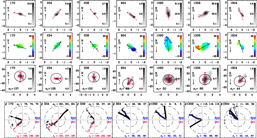
Figure 4: Top to bottom: Integrated intensity for CHVCs selected from HIPASS (Putman et al., 2002), velocity centroid maps, position-velocity plots, and derived position and inclination angles. Red arrows denote the direction of the cloud tail. Positions in $(GL,GB)$ are relative to the cloud’s catalogued coordinates. Letters $N$ and $S$ indicate Northern or Southern Galactic hemisphere. Black vertical arrows indicate whether the cloud is moving toward lower (downward) or higher $|z|$ (upward). Clouds approaching the observer ($\alpha_{i}<90^{\circ}$) are denoted by a dotted circle, otherwise by a “x”. The position axis in the pv-plots is counted from head to tail. Bottom row: Position angle $\alpha_{p}$ (black symbols, lines) and inclination angle $\alpha_{i}$ (blue or red symbols, lines). Both angles $\alpha_{p}$ and $\alpha_{i}$ are counted counter-clockwise from the top, with $0\leq\alpha_{p}\leq 360$ and $0\leq\alpha_{i}\leq 180$. Long dashed circles indicate $S/N$ values of $20$ and $40$. Solid lines refer to the median value, short dashed lines to the lower and upper quartile. These values are given also at the top and bottom of each panel (lower quartile, median, upper quartile). The horizontal dashed line separates inclination angles for approaching (blue) and receding (red) CHVCs.

We determine the angles $\alpha_{p}$ and $\alpha_{i}$ for a sequence of increasing signal-to-noise values ($S/N=[5,40]$ in steps of $1$). For $S/N<5$, angle estimates were generally unreliable in our sample. The bottom row of Fig. 4 summarises the derived angles for the selected CHVCs. Shown are the median values (solid lines) including lower and upper quartiles (dashed lines), to highlight the uncertainties in the angle estimates. The position angle $\alpha_{p}$ can be determined within $<\pm 3^{\circ}$ (exception: cloud 1804, whose position angle “drifts” with $S/N$). For well-defined clouds, the inclination angles show similar ranges. To further assess the reliability of the angle estimates, we calculate $\alpha_{i}$ for all $0\leq\alpha_{p}\leq 360$ and for all $S/N$. In the resulting map of $\alpha_{i}(\alpha_{p},S/N)$ we search for “consistent” $\alpha_{i}$ values, i.e. for regions in $(\alpha_{p},S/N)$ space across which $\alpha_{i}$ does not change by more than $2^{\circ}$. These regions are usually extended over a large range in $S/N$, while for inconsistent solutions, $\alpha_{i}$ varies strongly with $\alpha_{p}$. The largest of these regions is taken as the solution. The resulting angle estimates are consistent with the direct fits described above.

4 Discussion

4.1 A Method to Constrain CHVC Distances

We explore whether the full cloud orientation can be used to derive distance constraints of CHVCs via the velocity of a CHVC relative to its background medium, $v_{rel}$. This requires several assumptions. It is not our intent that these be necessarily correct, but that they are sufficiently plausible to outline the method. The goal is to calculate $v_{rel}=|\mathbf{v}_{tot}-\mathbf{\Theta}|$ along the line-of-sight at a given $(GL,GB)$ for a range of distances $D$. Here, $\mathbf{v}_{tot}$ is the three-dimensional velocity of the CHVC in Galactic cartesian coordinates, and $\mathbf{\Theta}$ is the three-dimensional (halo) rotation velocity of the background medium. All velocities are relative to the Galactic Standard of Rest (GSR). Since $\mathbf{v}_{tot}$ is constant along the line-of-sight, but $\mathbf{\Theta}$ will change with $D$, $v_{rel}=v_{rel}(D)$. If we have additional information on $v_{rel}$, such as a terminal velocity $v_{max}$ at which CHVCs can move with respect to the background medium, distances $D$ can be identified for which $v_{rel}\leq v_{max}$.

Setting $\mathbf{\Theta}$ requires a Galactic halo rotation model. For demonstration, we combine the rotation curve model of Fich et al. (1989) with an exponential drop-off in $z$, reproducing the linear gradient of $-22$ km s^-1 derived by Levine et al. (2008). Our halo rotation model then reads as

$$|\mathbf{\Theta}|\equiv v_{R}(R_{xy},z)=(109+108R_{xy}^{0.0042})\,e^{-|z|/10},$$ (5)

with $R_{xy}$ and $z$ in kpc. The radius $R_{xy}$ gives the Galactocentric distance in the plane, with the full Galactocentric radius being $R=(R^{2}_{xy}+z^{2})^{1/2}$.

There are several options to constrain $v_{rel}$, such as setting $v_{max}$ to the terminal velocity due to hydrodynamical drag (Benjamin & Danly, 1997), estimating $v_{rel}$ based on differential drag analysis of the CHVC (Peek et al., 2007), or limiting $v_{max}$ to the sound speed of the background medium for sufficiently diffuse CHVCs. Based on our models (Heitsch & Putman, 2009), we choose the latter and set $v_{max}=c_{s}=100$ km s^-1. Other options will be explored in a future contribution.

Table 1 summarises the estimated parameters for the seven CHVCs shown in Fig. 4 together with a few other CHVCs selected from HIPASS. Roughly $50$% of the sample CHVCs have near distance constraints (at $c_{s}=100$ km s^-1). Most remaining CHVCs show relative velocities $v_{rel}>200$ km s^-1, and thus do not lead to a distance constraint. The value of $|\mathbf{v}_{tot}|$ depends strongly on $\alpha_{i}$: At $\alpha_{i}=90,270^{\circ}$, $|\mathbf{v}_{tot}|$ cannot be reconstructed.

Though none of the observed CHVCs have (previous) direct distance constraints, many of them are potentially related to larger HVC complexes with constraints from their position-velocity proximity (Peek et al., 2008; Putman et al., 2011). In the Southern sky, the majority of the HVCs (and the CHVCs in Table 1) can be associated with the Magellanic System and though the distance to the Magellanic complexes are unknown, the Magellanic Clouds themselves are at $50$-$60$ kpc and the associated clouds are expected to be further away than the lower distance limits $D_{lo}$ in Table 1. One strong comparison point in our sample is cloud 238, which is in the position-velocity vicinity of the tail of Complex C. Complex C has a direct distance constraint of $10$ kpc (Thom et al., 2008), and we find this cloud has a lower distance estimate of $10$ kpc. Within the uncertainties, the results of the method are thus far consistent with existing distance constraints.

Table 1: Selected HIPASS CHVC parameters. [1] HIPASS number. [2] Galactic longitude GL. [3] Galactic latitude GB. [4] Position angle $\alpha_{p}$. [5] Inclination angle $\alpha_{i}$. [6] Lower distance limit $D_{lo}$. [7] Total velocity $|\mathbf{v}_{tot}|$. [8] Cloud approaching ($\odot$) or receding ($\otimes$), and moving toward ($\downarrow$) or away from ($\uparrow$) disk. [9] Possible association with known HVC complexes. Complexes in square brackets do not have distance constraints. For identification of the HVC complexes, see Kalberla & Haud (2006); Putman et al. (2012).

[1]	[2]	[3]	[4]	[5]	[6]	[7]	[8]	[9]
170	$16.8$	$-25.0$	$73$	$138$	$-$	$240$	$\otimes\uparrow$	GCN
234	$24.5$	$-1.8$	$321$	$127$	$-$	$324$	$\otimes\uparrow$	GCN
238	$24.8$	$8.8$	$37$	$152$	$10.0$	$24$	$\otimes\downarrow$	C
924	$258.5$	$-39.1$	$56$	$39$	$21.7$	$85$	$\odot\uparrow$	LA
1093	$271.0$	$10.8$	$8$	$50$	$20.9$	$72$	$\odot\downarrow$	LA
1308	$285.0$	$-16.1$	$118$	$68$	$22.4$	$2$	$\odot\downarrow$	LA
1804	$334.8$	$30.7$	$20$	$44$	$-$	$234$	$\odot\downarrow$	L
48	$3.9$	$-63.7$	$70$	$124$	$-$	$270$	$\otimes\uparrow$	MS?
200	$21.2$	$-61.2$	$236$	$24$	$12.3$	$59$	$\odot\downarrow$	MS?
632	$224.1$	$-17.0$	$8$	$139$	$24.0$	$81$	$\otimes\uparrow$	MS?
648	$226.6$	$-33.4$	$90$	$25$	$7.7$	$27$	$\odot\uparrow$	MS?
1221	$279.1$	$-16.7$	$211$	$49$	$8.4$	$97$	$\odot\downarrow$	LA
1616	$316.9$	$-76.8$	$94$	$67$	$-$	$166$	$\odot\downarrow$	MS
1806	$335.0$	$16.1$	$191$	$50$	$29.4$	$41$	$\odot\uparrow$	[WD]

The weakest link in these distance constraints is the choice of a halo rotation model. Increasing the characteristic scale from $10$ to $20$ kpc in equation 5 (and thus flattening the drop-off of $\mathbf{\Theta}$ with $z$) increases all the distance constraints by a factor of $\sim 2$. Halo rotation models without $z$-dependence (Hodges-Kluck et al., 2016) do not yield results if we assume $v_{rel}\lesssim 100$ km s^-1. We interpret this as a limitation of our assumptions regarding $v_{rel}$ rather than a limitation of the method itself.

4.2 Caveats

Residual Fitting Correcting the inclination angle estimate (equation 3) by fitting the residuals raises the question about the physical motivation for equation 4. Equation 3 assumes that the velocity gradient along the tail, caused by deceleration of the cloud gas, is linear. This is not necessarily correct (Brüns et al., 2001; Peek et al., 2007, see also Fig. 2); material directly behind the cloud is expected to travel nearly at the same velocity as the cloud. Velocities close to the cloud speed reduce the velocity asymmetry $a_{v}$, thus overestimating $\alpha_{i}$. The fit parameters might also depend on environmental factors, such as the ambient density, and the absolute cloud velocity. These dependencies and their quantification can only be explored with a larger model grid, which is beyond the scope of this paper.

Effect of Background Flow on $\alpha_{i}$ Since the CHVCs in our sample are identified via HI emission, their $\alpha_{i}$ estimates rest on the assumption that the neutral gas interacts directly with the background halo. Yet, there is evidence for substantial ionized envelopes co-moving with HVCs (Hill et al., 2009; Lehner et al., 2009, 2012). For a CHVC moving at a velocity $|\mathbf{v}_{tot}|=v_{rel}+v_{env}$ with respect to an ionized envelope traveling in the same direction at $v_{env}$, the reduced drag results in a smaller spread along the velocity axis in the position-velocity plot, and therefore in a pitch angle biased toward $90^{\circ}$. This in turn increases the inferred total velocity $\mathbf{v}_{tot}$. On the other hand, the observed radial velocity combines the line-of-sight component of the HI CHVC and the ionized envelope. Therefore, our method tends to overestimate $|\mathbf{v}_{tot}|$ if the CHVC is moving within a larger ionized envelope. Yet, if the line-of-sight component of the envelope’s velocity – and therefore the line-of-sight component of $v_{rel}$ – is known, the velocity spread in the position-velocity plot correctly refers to $v_{rel}$, and thus $\alpha_{i}$ is not affected by the ionized envelope.

Effects of Cloud Evolution on $\alpha_{i}$ The interaction of the CHVC with the ambient gas leads to turbulent structures, and occasionally to large “chunks” of the cloud being ripped off. Such “secular” events can affect the estimates for $\alpha_{i}$ and $\alpha_{p}$. The strong time variations in the residuals of $\alpha_{i}$ (Fig. 3b,d) are caused by this effect.

The $\alpha_{i}$ estimate relies on the translation of the effect of the hydrodynamic drag on the CHVC’s tail into centroid velocity profiles. The method assumes a monotonic centroid velocity profile, i.e. for a cloud moving at an angle toward the observer, the head would have the most negative velocities, and the tail the most positive ones. Yet, the centroid velocity map of Fig. 2 demonstrates that this need not be the case (also Brüns et al., 2001). The swath of “green” (less negative) velocities at the head of the cloud is caused by material flowing around the cloud away from the observer.

5 Summary

We present a method to determine the three-dimensional orientation of CHVCs. The inclination angle is derived from asymmetries in the intensity distribution of a CHVC’s position-velocity plot (Figs. 2 and 4). We test the method with the help of numerical simulations of CHVCs and identify possible systematic effects on the inclination angle estimate. When applied to CHVCs drawn from HIPASS, the method is returning results that are stable with increasing signal-to-noise. The method can be improved by a more detailed analysis of the position-velocity plots, and by a more rigorous statistical treatment. Applications to clouds being ablated in other astrophysical environments seem obvious.

We discuss the possibility to constrain distances by assuming a limiting CHVC velocity with respect to the background medium. Such a limit constrains the possible locations of a CHVC along its line-of-sight, given a Galactic halo rotation model. We find lower distance limits for $\sim 50$% of the selected HIPASS CHVC sample. The estimates are consistent with previous distance constraints.

References

- Benjamin & Danly (1997) Benjamin R. A., Danly L., 1997, ApJ, 481, 764
- Bland-Hawthorn & Putman (2001) Bland-Hawthorn J., Putman M. E., 2001, in Hibbard J. E., Rupen M., van Gorkom J. H., eds, Astronomical Society of the Pacific Conference Series Vol. 240, Gas and Galaxy Evolution. p. 369 (arXiv:astro-ph/0110043)
- Brüns et al. (2000) Brüns C., Kerp J., Kalberla P. M. W., Mebold U., 2000, A&A, 357, 120
- Brüns et al. (2001) Brüns C., Kerp J., Pagels A., 2001, A&A, 370, L26
- Fich et al. (1989) Fich M., Blitz L., Stark A. A., 1989, ApJ, 342, 272
- Fox et al. (2016) Fox A. J., et al., 2016, ApJ, 816, L11
- Heitsch & Putman (2009) Heitsch F., Putman M. E., 2009, ApJ, 698, 1485
- Hill et al. (2009) Hill A. S., Haffner L. M., Reynolds R. J., 2009, ApJ, 703, 1832
- Hodges-Kluck et al. (2016) Hodges-Kluck E. J., Miller M. J., Bregman J. N., 2016, ApJ, 822, 21
- Jin (2010) Jin S., 2010, MNRAS, 408, L85
- Kalberla & Haud (2006) Kalberla P. M. W., Haud U., 2006, A&A, 455, 481
- Lehner et al. (2009) Lehner N., Staveley-Smith L., Howk J. C., 2009, ApJ, 702, 940
- Lehner et al. (2012) Lehner N., Howk J. C., Thom C., Fox A. J., Tumlinson J., Tripp T. M., Meiring J. D., 2012, MNRAS, 424, 2896
- Levine et al. (2008) Levine E. S., Heiles C., Blitz L., 2008, ApJ, 679, 1288
- Lockman et al. (2008) Lockman F. J., Benjamin R. A., Heroux A. J., Langston G. I., 2008, ApJ, 679, L21
- Olano (2008) Olano C. A., 2008, A&A, 485, 457
- Peek et al. (2007) Peek J. E. G., Putman M. E., McKee C. F., Heiles C., Stanimirović S., 2007, ApJ, 656, 907
- Peek et al. (2008) Peek J. E. G., Putman M. E., Sommer-Larsen J., 2008, ApJ, 674, 227
- Putman et al. (2002) Putman M. E., et al., 2002, AJ, 123, 873
- Putman et al. (2003) Putman M. E., Bland-Hawthorn J., Veilleux S., Gibson B. K., Freeman K. C., Maloney P. R., 2003, ApJ, 597, 948
- Putman et al. (2011) Putman M. E., Saul D. R., Mets E., 2011, MNRAS, 418, 1575
- Putman et al. (2012) Putman M. E., Peek J. E. G., Joung M. R., 2012, ARA&A, 50, 491
- Richter et al. (2015) Richter P., de Boer K. S., Werner K., Rauch T., 2015, A&A, 584, L6
- Saul et al. (2012) Saul D. R., et al., 2012, ApJ, 758, 44
- Stanimirović et al. (2006) Stanimirović S., et al., 2006, ApJ, 653, 1210
- Thom et al. (2006) Thom C., Putman M. E., Gibson B. K., Christlieb N., Flynn C., Beers T. C., Wilhelm R., Lee Y. S., 2006, ApJ, 638, L97
- Thom et al. (2008) Thom C., Peek J. E. G., Putman M. E., Heiles C., Peek K. M. G., Wilhelm R., 2008, ApJ, 684, 364
- Wakker (2001) Wakker B. P., 2001, ApJS, 136, 463
- Wakker & van Woerden (1997) Wakker B. P., van Woerden H., 1997, ARA&A, 35, 217
- Wakker et al. (2007) Wakker B. P., et al., 2007, ApJ, 670, L113