Characterizing HR 3549 B using SPHERE

Abstract

Aims. In this work, we characterize the low mass companion of the A0 field star HR 3549.

Methods. We observed HR 3549AB in imaging mode with the the NIR branch (IFS and IRDIS) of SPHERE@VLT, with IFS in $YJ$ mode and IRDIS in the H band. We also acquired a medium resolution spectrum with the IRDIS long slit spectroscopy mode. The data were reduced using the dedicated SPHERE GTO pipeline, purposely designed for this instrument. We employed algorithms such as PCA and TLOCI to reduce the speckle noise.

Results. The companion was clearly visible both with IRDIS and IFS. We obtained photometry in four different bands as well as the astrometric position for the companion. Based on our astrometry, we confirm that it is a bound object and put constraints on its orbit. Although several uncertainties are still present, we estimate an age of $\sim$100-150 Myr for this system, yielding a most probable mass for the companion of 40-50M_Jup and $T_{eff}\sim 2300-2400$ K. Comparing with template spectra points to a spectral type between M9 and L0 for the companion, commensurate with its position on the color-magnitude diagram.

1 Introduction

In recent years, a handful of giant planets and brown dwarfs have been discovered around young stars (with ages less than few hundreds of Myr) through the direct imaging technique (see e.g. Chauvin et al. 2005b, Chauvin et al. 2005a, Marois et al. 2008, Marois et al. 2010, Lagrange et al. 2010, Biller et al. 2010, Carson et al. 2013, Rameau et al. 2013, Bailey et al. 2014). However, it is difficult to characterize these objects, as they generally lack precision multiwavelength photometry and spectrometry. Thus, fundamental properties such as e.g. mass, radius, $T_{eff}$, $\log{g}$ and spectral type are often poorly constrained for these objects.

The low-mass companion to the main sequence A0 star HR 3549 (HIP 43620; HD 76346) is such an object. Discovered by Mawet et al. (2015a) in $L^{\prime}$-band observations with NACO at VLT, the detected companion was at a separation of $\sim$0.9 arcsec and at a position angle of $\sim$$157^{\circ}$ in the discovery epoch. HR 3549 has a parallax of 10.82$\pm$0.27 mas (van Leeuwen 2007) implying a distance of $\sim$92.5 pc. However, while the distance of the system is well-constrained, the host star has an estimated age between 50 and 400 Myr, leading to a wide range both for the mass estimation (between 15 and 90 M_Jup) and for the effective temperature of the companion (between 1900 and 2700 K). Thus, it was not possible to precisely infer the fundamental properties of the companion and it was generically identified as an L-type object. The parent star hosts a dust disk as well, based on a measured WISE infrared excess at 22 $\mu$m (W1-W4=0.56$\pm$0.06 mag) (Cutri et al. 2012; Mawet et al. 2015a). No excess was found at 12 $\mu$m, implying a temperature for the dust disk of 153 K and an outer disk radius of $\sim$17 AU from the host star, well inside the companion position.

In the last few years, a new generation of direct-imaging instruments have come online. These instruments provide both precise multiband photometry and low and medium resolution spectroscopic capabilities, enabling a better characterization of low-mass companions to young stars close to the Sun. SPHERE at the VLT is a member of this cohort of instruments (Beuzit et al. 2008) and started operations at the beginning of 2015. It is composed of three scientific modules operating both in the NIR with IRDIS (Dohlen et al. 2008) and IFS (Claudi et al. 2008), and in the visible with ZIMPOL (Thalmann et al. 2008). It is equipped with the SAXO extreme adaptive optics system (Fusco et al. 2006; Petit et al. 2014; Sauvage et al. 2014), with a 41$\times$41 actuators wavefront control, pupil stabilization, differential tip tilt control and employs stress polished toric mirrors for beam transportation (Hugot et al. 2012). In the main IRDIFS imaging mode, low resolution (R=50) spectra are obtained with the IFS between 0.95 and 1.35 $\mu$m while IRDIS is simultaneously used in dual-band imaging mode (DBI; Vigan et al. 2010) with the H23 filter pair (wavelength $H2$=1.587 $\mu$m; $H3$=1.667 $\mu$m). A lower resolution (R=30) spectrum but with a wider spectral coverage can be obtained when SPHERE is operating in the IRDIFS_EXT mode. In this mode, R=30 spectra are obtained with the IFS in the YH band between 0.95 and 1.65 $\mu$m while IRDIS is simultaneously used in dual-band imaging mode with the K12 filter pair (wavelength $K1$=2.110 $\mu$m; $K2$=2.251 $\mu$m). A more complete characterization of the companions can be carried out with IRDIS in the long slit spectroscopy (LSS) mode that supplies a medium resolution spectrum (MRS - R=350). In the past year, SPHERE has demonstrated its capability to characterize substellar companions in e.g. Maire et al. (2016), Vigan et al. (2016), Bonnefoy et al. (2016), Zurlo et al. (2016) and Bonnefoy (2015).

We observed HR 3549 with the NIR branch instruments of SPHERE in December 2015. In this paper we report our results on these observations. In Section 2 we describe observations and data reduction, in Section 3 we illustrate the results that are then discussed in Section 4. Finally, in Section 5 we provide our conclusions.

2 Observations and data reduction

HR 3549 was observed on December 19th 2015 with SPHERE operating in the IRDIFS mode. For both IRDIS and IFS the dataset was composed of 16 datacubes, each of them with 4 individual frames of 64 s exposure time. The IRDIS observations used a 4x4 pixels dithering pattern while no dithering was used for the IFS observation. To enable angular differential imaging (ADI; Marois et al. 2006a) technique, the field of view (FOV) was allowed to rotate during the observations. To maximize the rotation, we observed over the meridian passage of the star, for a total FOV rotation of $\sim$$32.5^{\circ}$. For both instruments, frames with the point spread function (PSF) off-centered with respect to the coronagraph and frames with four satellite spots symmetric with respect to the central star were also taken before and after the coronagraphic observations to allow proper flux calibration and centering of the frames with respect to the star. The use of satellite spots to define the center of an image was first proposed by Sivaramakrishnan & Oppenheimer (2006) and Marois et al. (2006b) and its use in SPHERE is explained in Langlois et al. (2013) and in Mesa et al. (2015). To avoid saturation, the off-centered frames were observed using a neutral density filter.

The same target was observed again in the night of December 27th 2015 with IRDIS operating in long slit spectroscopy (Vigan et al. 2008) mode. In this case the dataset was composed of 23 datacubes, each of them composed of 5 frames with an exposure time of 32 s. The sequence also included the acquisition of an off-axis reference PSF by moving the star off of the coronagraph. To avoid saturation, this off-axis PSF was acquired using a neutral density filter (see e.g. Vigan et al. 2015). We used IRDIS-LSS in MRS corresponding to R=350.

2.1 IRDIFS data reduction

Data reduction for the IFS data was performed following the procedure described in Mesa et al. (2015) and in Zurlo et al. (2014). We applied the appropriate calibrations (dark, flat, spectral positions, wavelength calibration and instrument flat) to create a calibrated datacube composed of 39 images of different wavelengths for each frame obtained during the observations. The calibrated datacubes were then registered and combined using the principal components analysis (PCA; e.g. Soummer et al. 2012) algorithm to implement both ADI and spectral differential imaging (SDI, Racine et al. 1999) to remove the speckle noise. For IRDIS, after the application of the appropriate calibrations (dark, flat and centering), the speckle subtraction was performed using both the PCA and the TLOCI (Marois et al. 2014) algorithms. For both IFS and IRDIS the data reduction was partly performed using the pipeline of the SPHERE data center hosted at OSUG/IPAG in Grenoble.

Given the contrast of the order of $10^{-4}$ and the separation larger than 0.8 arcsec, the companion is visible even in a simple de-rotated and stacked image. As will be discussed in the next Sections, this helps calibrate and account for companion self-subtraction produced by the PCA and TLOCI algorithms.

2.2 IRDIS/LSS data reduction

The LSS data was analyzed using the SILSS pipeline (Vigan 2016), which has been developed specifically to analyse IRDIS LSS data. The pipeline combines the standard ESO pipeline with custom IDL routines to process the raw data into a final extracted spectrum for the companion. After creating the static calibrations (background, flat field, wavelength calibration), the pipeline calibrates the science data and corrects for the bad pixels. It also corrects for a known issue of the MRS data, which produces a variation of the PSF position with wavelength because of a slight tilt ($\sim$1 degree) of the grism in its mount. To correct for this effect, the pipeline measures the position of the off-axis PSF in the science data as a function of wavelength, and shifts the data in each spectral channel by the amount necessary to compensate for the chromatic shift. All individual frames are calibrated independently for the two IRDIS fields.

After this calibration and correction step, the speckles are subtracted in the data following an approach based on the spectral differential imaging technique described in Vigan et al. (2008) and Vigan et al. (2012). The method has now been optimized to provide a better subtraction of the speckles: instead of constructing a simple reference of the stellar signal as the mean (or median) of all the spatial channels where the signal of the planet is not present, we use all spatial channels where there is no signal from the companion as reference, and subtract a linear combination of these references to each of the channels where the companion is present. To best reproduce and subtract the speckles, the coefficients for the linear combination are optimized on the areas where the signal of the companion is absent. In practice, this approach is similar to the locally-optimized combination of images (LOCI; Lafrenière et al. 2007) applied to LSS. This analysis is performed on all frames independently, and then the speckle-subtracted frames are median-combined. Since the wavelength calibration is slightly different for both IRDIS fields, we obtain a final frame for each of the two fields.

The extraction of the spectrum of the companion in both IRDIS fields is performed using a 1 $\lambda/D$-wide aperture in each spectral channel. The exact separation of the companion within the slit is known, but we optimized the position of the aperture so as to maximize the final integrated signal. The noise is measured by integrating the residual signal at a symmetric position with respect to the star, i.e. at a location where the speckles have been subtracted but where there is no companion signal. The spectrum of the off-axis reference PSF is extracted using an aperture of the same width. For the reference PSF, the effect of the neutral density filter is compensated in each spectral channel using a dedicated tool. The spectrum of the companion calibrated in contrast is then obtained by dividing its extracted spectrum by that of the off-axis reference PSF. Finally, the spectra obtained for each of the two IRDIS fields are interpolated on the same wavelength grid and averaged to increase the signal-to-noise ratio of the final spectrum.

2.3 Non SPHERE observations

We obtained photometric observations of HR 3549 over six nights between 3-26 March 2016 in order to measure its rotation period. We observed for four nights at the YSVP Observatory (Vale Park, South Australia, $-$34^∘53^′04^′′; 138^∘37^′51^′′E; 44 m a.s.l.) using a 23-cm Schmidt-Cassegrain telescope. We collected 1600 frames in the Johnson R-band filter, in defocused mode and with a per-frame exposure time of 1.3 s exposure. On each night, observations were collected for up to 8 consecutive hours, achieving an average photometric precision of $\sigma_{R}$ = 0.005 mag. We observed for two nights at the York Creek Observatory (YKO, Launceston, Tasmania, Australia, $-$41^∘06^′06^′′; 146^∘50^′33^′′E; 28 m a.s.l) using a 25-cm Takahashi Mewlon reflector. We collected 32 frames in the Johnson R-band filter, using 1 s exposures. Observations were collected for up to 5 consecutive hours, achieving an average photometric precision of $\sigma_{R}$ = 0.005 mag.

Bias subtraction, flat field correction, and aperture magnitude extraction were done using IRAF routines. We built an ensemble comparison star using four nearby stars that were found to have constant flux; Differential R-band magnitudes of HR 3549 were then obtained relative to this comparison star.

3 Results

3.1 IRDIFS

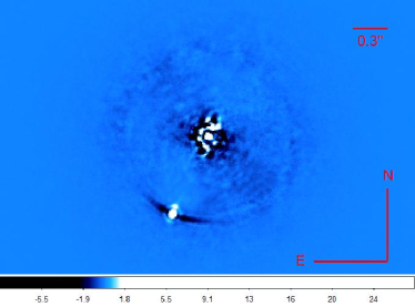
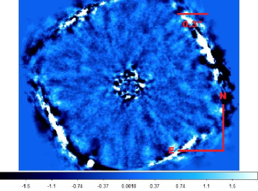
Figure 1: Left: Final image obtained with IRDIS.Right: Final image obtained with IFS.

In Figure 1 we display the final image obtained with IRDIS (left) and with IFS (right). While in both cases the companion is clearly visible, in the IFS case it is just at the edge of the instrument field of view (FOV), which introduces some difficulties in extracting photometry for this object. The companion position was measured by inserting negative scaled PSF images into the final image and shifting the simulated companion position until the standard deviation was minimized in a small region around the companion. This procedure was repeated in the final images obtained with differing numbers of principal components in the PCA analysis (as described in Section 2.1) and the error adopted on position was calculated as the standard deviation on these measures. The dominant error source is different for separation vs. position angle; the most important contribution to the the error on the separation is the uncertainty on the centering of the host star (assumed to be half of the pixel scale). On the other hand, the main contribution to the error on the position angle is the uncertainty on the position of the true north (TN), calculated by observing an astrometric calibration field. Astrometric measurements performed with IRDIS and IFS are listed in Table 1.

Table 1: Astrometric position for HR 3549 B.

Instrument	$\Delta$$\alpha$ (arcsec)	$\Delta$dec (arcsec)	Separation (arcsec)	Position angle
IFS	0.348$\pm$0.004	-0.776$\pm$0.004	0.850$\pm$0.006	155.8$\pm$0.5
IRDIS	0.344$\pm$0.007	-0.775$\pm$0.007	0.848$\pm$0.009	156.1$\pm$0.7

Exploiting our astrometric results we were able to extend the common proper motion analysis from Mawet et al. (2015a), further confirming that HR 3549 B is a bound object. The result of this analysis is shown in Figure 2. We interpret the small changes in projected separation and position angle with respect to Mawet et al. (2015a) as likely due to to orbital motion. The possible orbital solutions compatible with the data are discussed in Section 4.4.

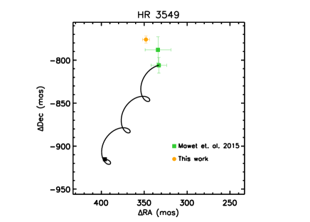
Figure 2: Common proper motion analysis for HR 3549 B. The black solid line displays the motion of the companion if it was a background object while the black square at the end of the line indicates the position that it would have at the observation date. The green points are taken from Mawet et al. (2015a), the orange one is from our astrometric measurements. We only plot astrometric values from the IFS observation, as our IFS observations provided a higher astrometric precision than our IRDIS observations.

In Table 2 we report the photometry obtained in four different bands using both IFS data for Y and J band and IRDIS data for H2 and H3 band taken as described in Section 2. IFS photometry was obtained by median combining all spectral channels between 0.95 and 1.15 $\mu$m for the Y band and between 1.15 and 1.35 $\mu$m for the J band. The error bars were calculated in a similar way, but do not incorporate the errors given by the uncertainty on the parallax given in Section 1. For this reason, an error of the order of 0.055 mag was to be added to the error bars listed in Table 2.

Table 2: Absolute magnitudes for HR 3548 B in four different spectral band from the IRDIFS data.

Y	J	H2	H3
$11.98\pm 0.16$	$11.06\pm 0.06$	$10.24\pm 0.07$	$10.14\pm 0.02$

The 5-$\sigma$ contrast curve derived from both IRDIS and IFS final images is shown in Figure 3 where the green line is the contrast obtained using IRDIS while the dashed orange line is the one obtained from IFS. At a separation of 0.5”, we obtained a contrast of the order of $\sim 1.6\times 10^{-6}$ ($\Delta$J$\sim$14.4) with the IFS and a contrast $\sim 3.2\times 10^{-6}$ ($\Delta$H$\sim$13.7) with IRDIS. At separations $>$1.3”, IRDIS achieves contrasts better than $10^{-6}$.

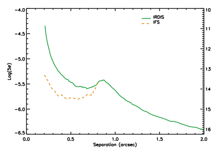
Figure 3: Contrast plot for our HR 3549 observations. IRDIS contrast is plotted with a green solid line while IFS contrast is plotted with an orange dashed line. The contrast for both instruments was obtained using the PCA algorithm.

As previously noted, the large separation and the relatively small contrast between the companion and the host star allowed us to see the companion in the calibrated datacube after only de-rotation and median-stacking. The PCA algorithm used to remove speckle noise does so at expense of removing some of the light from the companion (aka self-subtraction). Since the companion is easily retrieved without PCA in this case, we can use the simple de-rotated and median-stacked reduction to mitigate the effect of self-subtraction from the PCA algorithm.

Both LOCI and PCA algorithms build ideal PSFs and then subtract them from the data image. If these PSFs still contain light from the companion, then some of the flux of the companion will be removed in this subtraction. We thus build our PSFs in a way that avoids including light from the companion. For the region less than 1.5$\lambda$/D from the companion position, we replace the pixels in this region with the median value obtained for all the pixels outside this region but at the same separation from the central star (henceforth, the masked cube). We then create PSFs to be subtracted from this masked cube by applying the PCA algorithm. These PSFs are then subtracted from the original cube, thus preventing self-subtraction of the companion. The values obtained with this procedure and the value obtained from the unsubtracted datacube agree well. We evaluated the photometric error by applying the same procedure in ten different points at the same separation from the central star and calculating the standard deviation on these results. The same procedure was applied to the IRDIS data to obtain two more spectral points.

We converted our spectrum from contrast into flux by multiplying it by a flux calibrated BT-NEXTGEN (Allard et al. 2012) synthetic spectrum for the host star, adopting $T_{eff}$ = 10200 K $\log{g}$=4.0 and [M/H]=0.0. We justify this choice of $T_{eff}$ and metallicity in Section 4.1. Finally, we smooth this spectrum to R=50 to match the resolution of the IFS spectrum. Given that the resulting spectrum has poorer S/N and resolution than the LSS IRDIS spectrum presented in Section 3.2, we do not perform fits to it with template spectra or synthetic spectra. However, this spectrum matches the LSS spectrum quite well as it it showed in Figure 4.

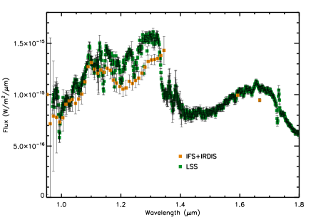
Figure 4: Comparison between the spectrum of HR3549 B obtained using IFS+IRDIS (orange squares) and the one obtained using LSS (green squares).

3.2 LSS

We applied the same procedure described for the IFS+IRDIS spectrum in the previous section to the IRDIS LSS spectrum (resolution of R=350). The spectrum was very noisy both at the short and long wavelength extremes, thus we used only only the range between 0.97 and 1.8$\mu$m, for 729 measurements at distinct wavelengths as opposed to the 780 original spectral points. We fit our final spectrum with spectra from both the Montreal Brown Dwarf and Exoplanet Library and the library from Allers & Liu (2013). We convolved each library spectrum to match that of our observed spectrum and interpolated to obtain flux values at the same wavelengths as are covered by our LSS spectrum. The spectral region between 1.35 and 1.45 $\mu$m is contaminated by a strong telluric absorption band; this spectral region was hence left out of our fit.

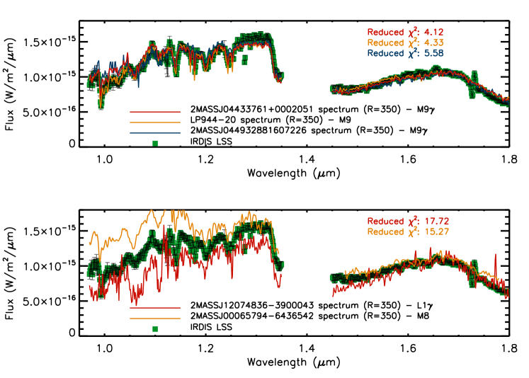
Figure 5: The LSS medium resolution (R=350) spectrum is displayed with green squares, with error bars shown for each spectrum value. The three best-fit spectra from the spectral libraries described in the text are also plotted. Lower panel: Similar to the upper panel, but with M8 and L1 spectra superimposed to illustrate the imperfect fit obtained in these cases.

In Figure 5 we display the medium (R=350) resolution spectrum obtained from the IRDIS LSS data. In the upper panel we display the three best-fit spectra. The best fit is obtained for a M9$\gamma$ (2MASSJ02103857-3015313 Gagné et al. 2015) and comparably good fits are obtained for two other M9 objects, specifically LP 944-20 (Allers & Liu 2013) and 2MASSJ044932881607226 (Gagné et al. 2015). In the lower panel of Figure 5 we display the fit of our spectrum alongside two spectra of different spectral type. In this case we used the L1 type object 2MASSJ12074836-3900043 (Gagné et al. 2015) and the M8 type object 2MASSJ00065794-6436542 (Gagné et al. 2015).

4 Discussion

4.1 Characteristics of HR 3549

According to the tables in Pecaut & Mamajek (2013), the colors of the host star agree well with its classification as an AO star. More precisely, if E(B-V)=0.00 is adopted, a spectral type of between a B9.5 and a A0 star is derived, but if E(B-V)=0.01 is adopted instead, the colors are closer to those of a B9.5 spectral type. This suggests that the reddening for this star is small, which is further confirmed by the polarization measures of $0.030\%\pm 0.030\%$ (Heiles 2000) and of $0.044\%\pm 0.022\%$ (Santos et al. 2011) for this star. While a unique relationship between polarization and reddening does not exist, we adopt a most probable relationship of $E(B-V)\sim$$P_{int}/5$ from Serkowski et al. (1975). This leads to $E(B-V)=0.006\pm 0.006$ from Heiles (2000) and $E(B-V)=0.009\pm 0.005$ from Santos et al. (2011). We thus adopt a best value for the reddening between 0.005 and 0.010 with an upper limit of 0.02. The impact of reddening on the spectral fit obtained in the previous Section is thus negligible.

4.1.1 Age of the HR 3549

A reliable determination of the age of the system is crucial for a proper characterization of the low mass component. However, as pointed out by Mawet et al. (2015a), the star is not associated with any known young moving group. Moreover, given its early spectral type, methods based on the activity, rotation and lithium abundance cannot be used to derive the age. We searched several catalogs (Tycho2, UCAC4, PPMXL, SPM4.0) for wide common proper motion companions within 30 arcmin from the star but did not identify any convincing candidates. Our kinematic analysis confirms the results by Mawet et al. (2015a); we also obtained space velocities U, V and W respectively of -16.7, -25.5 and -0.6 km/s. Therefore the space velocities of HR 3549 are well within the kinematic regions populated by young stars defined by Montes et al. (2001) and very close to the kinematic boundaries of the Nearby Young Population defined by Zuckerman & Song (2004). However, this result is not conclusive as several old stars also share these kinematic properties.

Therefore, we relied on isochrones fitting to derive the stellar age. We used the PARSEC models by Bressan et al. (2012) and the PARAM interface (version 1.3) (da Silva et al. 2006). This code uses as input the observational parameters (effective temperature, trigonometric parallax, apparent magnitude in V band, and metallicity along with their errors) to perform a Bayesian determination of the most likely stellar intrinsic properties, appropriately weighting all the isochrone sections which are compatible with the measured parameters. A flat distribution of ages was adopted as a prior for this analysis. The main stellar parameters obtained from our fits are listed in Table 3. The age reported in Table 3 obviously depends on the adopted metallicity. We assume [M/H]=0.00$\pm$0.10 as a reasonable estimate, since several studies have shown that the metallicity of young stars in the solar neighborhood is consistent with the solar value (see e.g. James et al. 2006; Santos et al. 2008; D’Orazi & Randich 2009; D’Orazi et al. 2011; Biazzo et al. 2011, 2012).

Our fit yields a most probable age of about 100-150 Myr, well within the range estimated by Mawet et al. (2015a). However, the oldest possible values from Mawet et al. (2015a) (300-400 Myr) are rejected by our fit.

4.1.2 Rotation of HR 3549

The non-SPHERE observations described in Section 2.3 were then used to define the rotation of HR 3549 using the following procedure. The time series of differential magnitudes was analyzed using the Lomb-Scargle (LS; Scargle 1982) and the CLEAN (Roberts et al. 1987) periodograms to search for possible periodicities. We found the same most significant power peak (significance level $>$99.9%) at P = 0.458$\pm$0.005 d in both LS and CLEAN periodograms, with a light curve amplitude of $\Delta$R = 0.008 mag. We consider this period as the stellar rotation period and attribute the slight rotational modulation to the presence of surface temperature inhomogeneities whose visibility is modulated by the stellar rotation. These results are displayed in Figure 6. These results are unsurprising, as there is significant evidence of the existence of a large fraction ($\sim$40%) of rotational variables among A type stars with light curve amplitudes up to a few hundredths of a magnitude (Balona 2016). When the stellar rotation period measured above is combined with the stellar radius R = 1.88 R_⊙ and the projected rotational velocity $v\sin{i}$ = 236$\pm$12 km s^-1 (Royer et al. 2002), we infer $\sin{i}$ = 1.13$\pm$0.1. Considering that HR 3549 is expected to host some level of surface magnetic activity, and the $v\sin{i}$ measurement is not corrected for the additional broadening effects of macro- and micro-turbulence, the estimated projected rotational velocity is likely an upper limit. Therefore, we can assume that HR 3549 is seen almost edge-on (i.e., $i$ $\sim$ 90^∘).

4.1.3 Separation of the disk

The data from the IR excess allow determination of an approximate lower limit on the separation of the disk from the star Indeed, having an excess at 22 $\mu$m and no excess at 12 $\mu$m we can consider the peak of the emission from the disk around 22 $\mu$m. Assuming a conservative error of 5 $\mu$m on the position of the peak we can obtain, using the Wien law, an approximate value for equilibrium temperature of the disk of $T_{eq}=131.7K$. From this value and assuming $T_{*}=10200$K and $R_{*}=1.88$R_⊙ we can calculate an approximate radius of the disk of $R_{disk}=22.3$. We can then assume a value around 20 AU for the lower limit of the disk radius.

Table 3: Stellar parameters obtained for HR 3549 from the isochrones fitting assuming two different values for E(B-V).

E(B-V)	$T_{\rm eff}$	Age (Gyr)	M/$M_{\odot}$	$\log{g}$	R/$R_{\odot}$
0.00	$10079\pm 200$	$0.152\pm 0.092$	$2.326\pm 0.071$	$4.228\pm 0.032$	$1.881\pm 0.064$
0.01	$10314\pm 200$	$0.121\pm 0.079$	$2.375\pm 0.070$	$4.243\pm 0.031$	$1.868\pm 0.062$

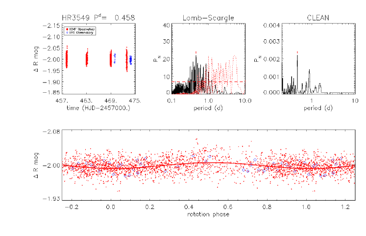
Figure 6: Top left panel: differential R-band magnitude time series of HR 3549. Top middle panel: LS periodogram. The dotted line represents the spectral window function. The horizontal dashed line is the power level corresponding to a 99.9% confidence level. Top right panel: CLEAN periodogram. Bottom panel: light curve phased with the P = 0.458d rotation period. The solid line is a sinusoidal fit with amplitude $\Delta$R = 0.008 mag.

4.2 Characterization of HR 3549 B

Using the photometry defined in Table 2 and exploiting the age range for the host star defined in Table 3, we were able to estimate the companion mass using the BT-Settl evolutionary model (Allard 2014). For our analysis we adopted five different ages, specifically 50, 100, 150, 200 and 300 Myr. While our age analysis finds a most probable age range of 100-150 Myr, younger and older ages cannot be completely excluded. Thus, we estimate mass for a broader range of ages here. The age of 300 Myr is marginal but has been included in this analysis for completeness. We estimate mass separately for all 4 spectral channels covered (Y and J band from IFS and H2 and H3 band from IRDIS, mass estimates presented given in Table 4). The mass determinations in different spectral channels agree well with each other. The companion mass ranges between $\sim$30 M_Jup in the case of a system age of 50 Myr and $\sim$70 M_Jup in the case of a system age of 300 Myr. However, as discussed above, we adopt a most probable age for the system of 100-150 Myr and thus a most probable mass for the companion of 40-50 M_Jup.

Table 4: Mass determinations for HR 3549 B. All masses are expressed in M_Jup.

Age (Myr)	Y	J	H2	H3
50	29	29	32	28
100	41	42	45	41
150	49	50	55	50
200	56	58	62	58
300	72	72	74	72

We estimate $T_{\rm eff}$ in a similar manner, with results presented in Table 5. Adopting the same range of ages as before, $T_{\rm eff}$ varies between $\sim$2180 K to $\sim$2500 K. The values obtained for different spectral bands are again in good agreement each other. For our most probable system age of 100-150 Myr, $T_{\rm eff}$ is between $\sim$2300 K and $\sim$2400 K.

Table 5: $T_{\rm eff}$ determinations for HR 3549 B. All temperatures are in K.

Age (Myr)	Y	J	H2	H3
50	2184	2181	2250	2134
100	2247	2263	2351	2249
150	2285	2310	2405	2307
200	2338	2365	2457	2364
300	2475	2485	2519	2488

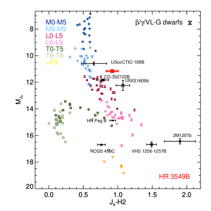
Figure 7: Color-magnitude diagram showing the position HR 3549 B relative to that of M, L and T field dwarfs and of young known companions. HR 3549 B is indicated by the red point.

In Figure 7 we compare the position of HR 3549 B on a color-magnitude diagram with the positions of M, L and T field dwarfs and young companions. The color-magnitude diagrams was generated using the synthetic SPHERE photometry of low gravity ($\beta$/$\gamma$/VL-G) dwarfs and old field MLTY dwarfs. This photometry was generated from the flux-calibrated near-infrared spectra of the sources gathered from the SpeXPrism library (Burgasser 2014), and additional studies (Patience et al. 2010; Allers & Liu 2013; Bonnefoy et al. 2014; Burgasser et al. 2010; Wahhaj et al. 2011; Gauza et al. 2015; Schneider et al. 2015, 2014; Gizis et al. 2015; Mace et al. 2013; Liu et al. 2013; Lafrenière et al. 2010; Delorme et al. 2008).

The position of HR 3549 B is indicated by a red point and lies at the transition between M and L dwarfs, thus confirming the spectral classification M9-L0 obtained in Section 3. However, the color of our object is redder than the field objects. This is in agreement with our estimation of an young age for this system (Kirkpatrick et al. 2008; Cruz et al. 2009; Schmidt et al. 2010).

4.3 Fitting with synthetic spectra

To further constrain the BD physical characteristics we fit its LSS spectrum with BT-Settl synthetic spectra models (Allard 2014). As with the template spectra, we choose to fit only the LSS medium resolution spectrum as it has significantly better S/N and resolution than the IFS+IRDIS spectrum. We again stress that the results obtained with the two different spectra are in excellent agreement. We have excluded the region between 1.35 and 1.45 $\mu$m from the fit due to the strong telluric water absorption feature at these wavelengths. In the upper panel of Figure 8 we display the three best fit synthetic spectra. The best fit in this case is obtained with a model with $T_{\rm eff}$=2300 K and $\log{g}$=5.0. Models with $T_{\rm eff}$=2400 K and $\log{g}$=5.5 and $T_{\rm eff}$=2300 K and $\log{g}$=4.5 produce comparably good fits to the spectrum. Thus, we adopt $T_{\rm eff}$=2350$\pm$100 K and $\log{g}$=5.0$\pm$0.5 for the companion. We integrated this model over all the wavelengths to calculate the total flux of our object, in order to obtain an estimate of the radius of the companion from Stefan-Boltzmann law. In this manner, we obtained a radius value of 1.13$\pm$0.17 R_Jup where the uncertainty is driven primarily by uncertainty on the $T_{\rm eff}$, while the error on the parallax is less important. The gravity and radius implied by our synthetic model fits exclude the youngest part of the 50-300 Myr age range considered above given that they mean that the companion is quite evolved. The value of $\log{g}$ in fact agrees well with what we would expect for an age of 100-150 Myr. In this age range, we estimate a mass range of 40-50 M_Jup (see Table 4), corresponding to $\log{g}$=4.89 and $\log{g}$=4.99 respectively. The temperature range of 2300-2400 K obtained from the model fit is also in good agreement with what we obtained for a 100-150 Myr object, as one can see from Table 5.

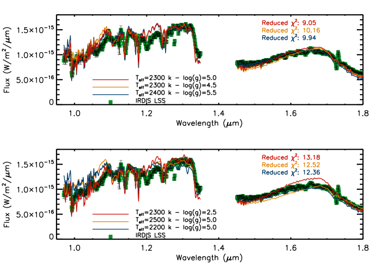
Figure 8: Three best fitting synthetic spectra superimposed with the HR 3549 B LSS medium resolution spectrum. Lower panel Same as the upper panel but including synthetic spectra with worse fits.

4.4 Orbit determination for HR 3549 B

We used the Least-Squares Monte-Carlo (LSMC) approach described in Ginski et al. (2013) to determine if we could constrain the orbit of the brown dwarf companion with the existing astrometry. To reduce the wide parameter space, we set the system mass to a fixed value of 2.35 M_⊙. This includes 2.3 M_⊙ for the primary star (Mawet et al. 2015b) and an average value of 0.05 M_⊙ for the companion. Note that the resulting orbital distributions are not highly sensitive to small changes in the companion mass. We further limited the semi-major axis to values smaller than 25.4 arcsec (2350 AU, 74.2 kyr period), following the criterion given in Close et al. (2003) for stability of the system against disruption in the galactic disk.

We then created 5$\times$10⁶ random sets of orbital elements. Samples were drawn from uniform distributions of each orbital parameter. Each of these sets of orbital elements was then used as starting point of a Least-Squares minimization routine using the Levenberg-Marquardt algorithm. We show the results of these 5$\times$10⁶ fitting runs in the lower left of Fig. 9. We include all solutions with a reduced $\chi^{2}$ smaller than 2. This rather large range was choosen to allow for potential systematic offsets between the astrometric measurements (i.e. due to different calibrators). This criterion is fulfilled by 433198 individual solutions. The three best fitting orbit solutions that we recovered are shown in Fig. 10, and their orbital parameters are listed in Tab. 6.

We find a large number of possible bound orbits that are compatible with the astrometric measurements. Specifically we find circular as well as eccentric orbits with eccentricities up to 0.993. It should be noted that it is of course quite common to find a large number of eccentric long period orbits that fit short orbital arcs without significant curvature.

In addition to the astrometric measurements, we consider the presence of an infrared excess of the host star to constrain the orbit of the companion. As seen in Section 4.1.3, the infrared excess of the star is best fit by the presence of a circumstellar debris disk with a lower limit for the radius up to $\sim$20 AU. We use the formulas given by Holman & Wiegert (1999) to compute the critical semi-major axis for dynamical stability of additional objects in the system given the eccentricity of an orbit solution below which the companion would disrupt the disk. We have to stress that the mass ratio of HR 3549 is slightly outside the range over which the Holman & Wiegert (1999) relationship were defined. However, detailed investigation of the dynamical stability of additional bodies for the three best fit orbits listed in Table 6 was performed using the frequency map analysis (FMA) technique as in Marzari et al. (2005), resulting in stability limits about 30% larger than the Holman & Wiegert (1999) equation. We then exclude all the orbits that do not fulfill this conditions. The result is shown in the upper right of Fig. 9. Our best fitting orbit is indeed not compatible with the presence of this inferred disk as is indicated in Fig. 10. Since we only infer the presence of the circumstellar disk and its outer radius from unresolved photometry, we first discuss the orbital parameter distribution of the companion without the constraints introduced by the disk.

4.4.1 Orbit without disk constraints

If the companion has formed in-situ, either via gravitational instability in the protoplanetary disk or star-like via collapse in the protostellar cloud, we would in principle expect a low orbital eccentricity. We indeed recover a large number of circular orbits. The inclination of circular orbits can already be constrained between 101.4 deg and 137.5 deg and orbital periods between 509 yr and 2579 yr. In addition, the longitude of the ascending node $\Omega$ can be constrained to two peak values close to 0 or 180 deg for the circular case.

On the other hand eccentric orbits might be a sign that the companion formed in a different part of the system and later experienced dynamic interaction with either an additional companion or a close encounter with another stellar object. Of course high eccentricities could also be explained in other ways, e.g. the companion could have formed outside of the system and was later captured. We find a large number of such eccentric orbits. In fact all our best fitting orbits shown in Fig. 10 are highly eccentric. In general eccentric solutions fit the current astrometric data set better than circular orbits. If we limit the sample of relevant orbits to fits with a reduced $\chi^{2}$ smaller than 1, then we find a minimum eccentricity of $\sim$0.3.

With increasing eccentricity the semi-major axis typically increases as well to fit the astrometric data points, up to our upper limit for the semi-major axisof 25.4 arcsec. However, there is also a large number of highly eccentric orbit solutions with short orbital periods that we can not yet exclude. We observe a peak of the eccentricity at a value of $\sim$0.65. Indeed the majority of orbit solutions at this eccentricity peak have small semi-major axes of $\sim$0.9 arcsec (83.2 AU, 495 yr period), but orbits with semi-major axes up to 13 arcsec, can not be excluded. The range of possible inclinations for orbits at this eccentricity peak goes from 96.7 deg to 180 deg, i.e. is significantly wider than for circular orbits. The longitude of the ascending node becomes essentially unconstrained at this point as well.

To distinguish between potential formation scenarios for the brown dwarf companion, it is important to check if the inclinations of its potential orbits are compatible with the inclination of the stellar spin axis. One would expect that an object that formed in-situ in the protoplanetary disk would show a similar inclination of its orbit as the stellar spin axis, while this is not necessarily true for an object that formed in a star-like fashion. Considering our conclusions about the value of $\sin{i}$ in Section 4.1, we would expect highly inclined orbits for the companion if its orbit is indeed aligned with the stellar spin. As discussed earlier and also as noted in Fig. 9, we indeed recover a range of such highly inclined orbits (circular and eccentric). We can thus conclude that the current astrometry is consistent with in-situ formation scenarios of the companion in the protoplanetary disk. However, we also find a variety of orbit solutions that are also consistent with other formation scenarios.

Continued astrometric monitoring of this object over the next decade might shed some light on its formation history, especially if significant orbit curvature is detected. However, it will be very difficult if impossible to disentangle different potential orbits via observation in the next few years. For example, our current estimates suggest that we would have to wait until 2060 to fully distinguish between the three best fit orbits listed in Table 6. On the other hand, new observations could help in narrowing down the parameter space for the companion.

4.4.2 Orbit with disk constraints

If we consider the presence of the circumstellar debris disk (outer radius of $\sim$20 AU), we can further constrain the orbital parameters of the companion. In the presence of the disk, highly eccentric orbits can not have arbitrarily small semi-major axes, since the companion would then disrupt the disk at periastron passage. One immediate consequence is that the peak that we find at an eccentricity of $\sim$0.65 vanishes completely. This is not surprising given that most of the orbital solutions in this eccentricity range had small semi-major axes of only $\sim$0.9 arcsec (83.2 AU, 495 yr period). The maximum eccentricity that we recover is 0.925 compared to 0.993 for the unconstrained case. As is seen in Fig. 9 we lose the ”steeper” branch of the semi-major axis - eccentricity distribution beyond an eccentricity of $\sim$0.5.

The inclination can be constrained as well with 99.5% of all solutions now located between 96.4 deg and 140 deg. This is highly consistent with the range of possible inclinations that we find considering the possible inclinations of the stellar spin axis, and might be an indication that the inclination of the companion orbit and the stellar spin axis are indeed aligned. Finally we can also constrain the longitude of the ascending node to values of 192.2$\pm$7.2 deg ($\pm$180 deg depending on the radial velocity of the companion).

Further astrometric monitoring of the system over the next decade will significantly improve our understanding of the orbit of this companion and will thus enable us to understand formation scenarios for this interesting system.

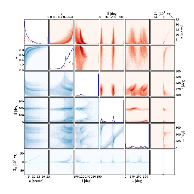
Figure 9: Result of our LSMC orbit evaluation. On the diagonal the distribution for each individual orbit parameter is shown, while the other tiles show correlations between two orbit parameters. On the lower left in a blue hue we show all orbit solutions with a reduced $chi^{2}$ smaller than 2, out of 5$\times$10⁶ orbit fits. On the upper right in a red hue we show all the solutions that are compatible with the presumed stable circumstellar disk.

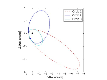
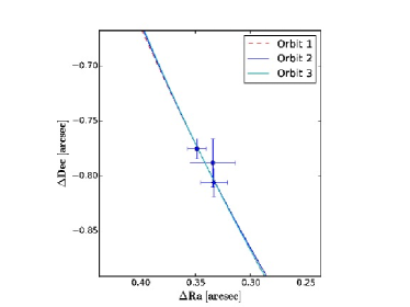
Figure 10: Left: Top 3 best-fitting orbits out of 5$\times$10⁶ runs of our LSMC fit for a mass of 1.22 M_⊙. Solid lines represent the apparent orbits. Here the red dashed lines represents best fitting orbits that are not compatible with the presence of the disk while the blue lines represents orbit compatible with the disk. Right: Same image zoomed in on the data points. The corresponding orbit elements are listed in Table 6.

Table 6: Orbit elements and $\chi^{2}_{red}$ of the best-fitting orbits shown in Fig. 10.

Nr.	1	2	3
a [arcsec]	4.77	3.24	1.44
a [AU]	441.2	299.7	133.2
e	0.88	0.69	0.56
P [yr]	6034.6	3383.8	1002.3
i [deg]	134.3	123.1	135.0
$\Omega$ [deg]	53.9	182.9	26.1
$\omega$ [deg]	0	63.9	336.8
T0 [yr]	2103.7	2042.5	2111.3
$\chi^{2}_{red}$	0.294	0.294	0.294

4.5 Mass limits for other objects in the system

Using our derived contrast curve (Figure 3), adopting our optimal age range of 100-150 Myr (see Section 4.3), and converting from contrast to mass using the Cond-Ames models, we set upper limits on the possible masses of other components of the system. The final result of this analysis is displayed in Figure 11 where we show the mass limit obtained both for IRDIS and IFS at three different possible system ages: 100, 150 and 200 Myr. While our previous analysis favours an age of 100-150 Myr, we included the 200 Myr age here as a conservative case. For all the considered ages, both IFS and IRDIS exclude the existence of any other sub-stellar objects with a mass larger than $\sim$13M_Jup at separation less than 0.8 arcsec. For an age of 100 Myr, we can exclude the presence of $>$9M_Jup objects at 0.5 arcsec from our IFS observations. From our IRDIS observations, we can exclude the presence of objects with mass larger than 10M_Jup at separation greater than 1 arcsec.

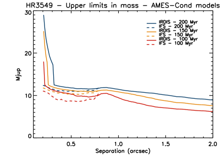
Figure 11: Upper limits for possible additional components of the system versus separation from the central star. Different ages are assumed: 200 Myr (blue line), 150 Myr (orange line) and 100 Myr (red line). We display both upper limit obtained with IRDIS (solid lines) and IFS (dashed lines).

5 Conclusions

We present here SPHERE observations of the star HR 3549, recovering the low mass companion discovered by Mawet et al. (2015a) both with IFS and IRDIS. We obtained precise astrometry and photometry in 4 bands for the companion. Our astrometry further confirms that the companion is bound to its host star. Significant uncertainty is still present in the age of this system. Assuming a conservative age range of 50-300 Myr combined with our multiband photometry, we estimate a mass range for this companion of $\sim$30-70 M_Jup and a $T_{\rm eff}$ range between $\sim$2200 and $\sim$2500 K. However, the position of this companion in the color-magnitude diagram as well as isochrone fitting strongly suggests that this system is young (100-150 Myr), thus, the most probable mass of the companion is between 40-50 M_Jup while its $T_{\rm eff}$ is probably between 2300-2400 K. This latter values are further confirmed by fits with BT-Settl synthetic spectra. Our best fit BT-Settl model has $T_{\rm eff}$=2300 K and $\log{g}$=5.0 but a comparably good fit is obtained with $T_{\rm eff}$=2400 K and $\log{g}$=5.0. The BT-Settl fits agree well with the $T_{\rm eff}$ and mass determination obtained from the object photometry.

Fitting both the IFS+IRDIS and medium resolution IRDIS LSS spectra for this object yielded a spectral type of M9-L0, right at the transition between M and L dwarf. The M/L transition spectral type is further confirmed by the position of the companion on the color-magnitude diagram.

The astrometric position obtained from our analysis together with the two earlier positions from Mawet et al. (2015a) allowed us to simulate a suite of potential orbits and thus constrain the companion’s orbital parameters. While the time span from these three astrometric points is too small to definitively measure any orbital parameters, we were however able to exclude families of orbits. The current astrometry is consistent with in-situ formation scenarios for the companion within the protoplanetary disk. However, we also find a variety of orbit solutions that are more consistent with other formation scenarios. Continued astrometric monitoring of this object over the next decade might shed some light on its formation history, especially if significant orbit curvature is detected. SPHERE will be a very valuable instrument for this continued astrometric monitoring.

Moreover, new data (for instance, the GAIA first data release) will better define the age of the system, thus allowing us to place tighter constraints on the physical charateristics of HR 3549 B.

This research has benefited from the Montreal Brown Dwarf and Exoplanet Spectral Library, maintained by Jonathan Gagné.

SPHERE is an instrument designed and built by a consortium consisting of IPAG (Grenoble, France), MPIA (Heidelberg, Germany), LAM (Marseille, France), LESIA (Paris, France), Laboratoire Lagrange (Nice, France), INAF– Osservatorio di Padova (Italy), Observatoire de Genève (Switzerland), ETH Zurich (Switzerland), NOVA (Netherlands), ONERA (France) and ASTRON (Netherlands), in collaboration with ESO. SPHERE was funded by ESO, with additional contributions from CNRS (France), MPIA (Germany), INAF (Italy), FINES (Switzerland) and NOVA (Netherlands). SPHERE also received funding from the European Commission Sixth and Seventh Framework Programmes as part of the Optical Infrared Coordination Network for Astronomy (OPTICON) under grant number RII3-Ct-2004-001566 for FP6 (2004-2008), grant number 226604 for FP7 (2009-2012) and grant number 312430 for FP7 (2013-2016).

References

- Allard (2014) Allard, F. 2014, in IAU Symposium, Vol. 299, Exploring the Formation and Evolution of Planetary Systems, ed. M. Booth, B. C. Matthews, & J. R. Graham, 271–272
- Allard et al. (2012) Allard, F., Homeier, D., & Freytag, B. 2012, Philosophical Transactions of the Royal Society of London Series A, 370, 2765
- Allers & Liu (2013) Allers, K. N. & Liu, M. C. 2013, ApJ, 772, 79
- Bailey et al. (2014) Bailey, V., Meshkat, T., Reiter, M., et al. 2014, ApJ, 780, L4
- Balona (2016) Balona, L. A. 2016, MNRAS, 457, 3724
- Beuzit et al. (2008) Beuzit, J.-L., Feldt, M., Dohlen, K., et al. 2008, in Society of Photo-Optical Instrumentation Engineers (SPIE) Conference Series, Vol. 7014, Society of Photo-Optical Instrumentation Engineers (SPIE) Conference Series, 18
- Biazzo et al. (2012) Biazzo, K., D’Orazi, V., Desidera, S., et al. 2012, MNRAS, 427, 2905
- Biazzo et al. (2011) Biazzo, K., Randich, S., Palla, F., & Briceño, C. 2011, A&A, 530, A19
- Biller et al. (2010) Biller, B. A., Liu, M. C., Wahhaj, Z., et al. 2010, ApJ, 720, L82
- Bonnefoy (2015) Bonnefoy, M. 2015, in AAS/Division for Extreme Solar Systems Abstracts, Vol. 3, AAS/Division for Extreme Solar Systems Abstracts, 203.05
- Bonnefoy et al. (2014) Bonnefoy, M., Chauvin, G., Lagrange, A.-M., et al. 2014, A&A, 562, A127
- Bonnefoy et al. (2016) Bonnefoy, M., Zurlo, A., Baudino, J. L., et al. 2016, A&A, 587, A58
- Bressan et al. (2012) Bressan, A., Marigo, P., Girardi, L., et al. 2012, MNRAS, 427, 127
- Burgasser (2014) Burgasser, A. J. 2014, in Astronomical Society of India Conference Series, Vol. 11, Astronomical Society of India Conference Series
- Burgasser et al. (2010) Burgasser, A. J., Simcoe, R. A., Bochanski, J. J., et al. 2010, ApJ, 725, 1405
- Carson et al. (2013) Carson, J., Thalmann, C., Janson, M., et al. 2013, ApJ, 763, L32
- Chauvin et al. (2005a) Chauvin, G., Lagrange, A.-M., Dumas, C., et al. 2005a, A&A, 438, L25
- Chauvin et al. (2005b) Chauvin, G., Lagrange, A.-M., Zuckerman, B., et al. 2005b, A&A, 438, L29
- Claudi et al. (2008) Claudi, R. U., Turatto, M., Gratton, R. G., et al. 2008, in Society of Photo-Optical Instrumentation Engineers (SPIE) Conference Series, Vol. 7014, Society of Photo-Optical Instrumentation Engineers (SPIE) Conference Series
- Close et al. (2003) Close, L. M., Siegler, N., Freed, M., & Biller, B. 2003, ApJ, 587, 407
- Cruz et al. (2009) Cruz, K. L., Kirkpatrick, J. D., & Burgasser, A. J. 2009, AJ, 137, 3345
- Cutri et al. (2012) Cutri, R. M., Skrutskie, M. F., van Dyk, S., et al. 2012, VizieR Online Data Catalog, 2281
- da Silva et al. (2006) da Silva, L., Girardi, L., Pasquini, L., et al. 2006, A&A, 458, 609
- Delorme et al. (2008) Delorme, P., Delfosse, X., Albert, L., et al. 2008, A&A, 482, 961
- Dohlen et al. (2008) Dohlen, K., Langlois, M., Saisse, M., et al. 2008, in Society of Photo-Optical Instrumentation Engineers (SPIE) Conference Series, Vol. 7014, Society of Photo-Optical Instrumentation Engineers (SPIE) Conference Series
- D’Orazi et al. (2011) D’Orazi, V., Biazzo, K., & Randich, S. 2011, A&A, 526, A103
- D’Orazi & Randich (2009) D’Orazi, V. & Randich, S. 2009, A&A, 501, 553
- Fusco et al. (2006) Fusco, T., Rousset, G., Sauvage, J.-F., et al. 2006, Opt. Express, 14, 7515
- Gagné et al. (2015) Gagné, J., Faherty, J. K., Cruz, K. L., et al. 2015, ApJS, 219, 33
- Gauza et al. (2015) Gauza, B., Béjar, V. J. S., Pérez-Garrido, A., et al. 2015, ApJ, 804, 96
- Ginski et al. (2013) Ginski, C., Neuhäuser, R., Mugrauer, M., Schmidt, T. O. B., & Adam, C. 2013, MNRAS, 434, 671
- Gizis et al. (2015) Gizis, J. E., Allers, K. N., Liu, M. C., et al. 2015, ApJ, 799, 203
- Heiles (2000) Heiles, C. 2000, AJ, 119, 923
- Holman & Wiegert (1999) Holman, M. J. & Wiegert, P. A. 1999, AJ, 117, 621
- Hugot et al. (2012) Hugot, E., Ferrari, M., El Hadi, K., et al. 2012, A&A, 538, A139
- James et al. (2006) James, D. J., Melo, C., Santos, N. C., & Bouvier, J. 2006, A&A, 446, 971
- Kirkpatrick et al. (2008) Kirkpatrick, J. D., Cruz, K. L., Barman, T. S., et al. 2008, ApJ, 689, 1295
- Lafrenière et al. (2010) Lafrenière, D., Jayawardhana, R., & van Kerkwijk, M. H. 2010, ApJ, 719, 497
- Lafrenière et al. (2007) Lafrenière, D., Marois, C., Doyon, R., Nadeau, D., & Artigau, É. 2007, ApJ, 660, 770
- Lagrange et al. (2010) Lagrange, A.-M., Bonnefoy, M., Chauvin, G., et al. 2010, Science, 329, 57
- Langlois et al. (2013) Langlois, M., Vigan, A., Moutou, C., et al. 2013, in Proceedings of the Third AO4ELT Conference, ed. S. Esposito & L. Fini, 63
- Liu et al. (2013) Liu, M. C., Magnier, E. A., Deacon, N. R., et al. 2013, ApJ, 777, L20
- Mace et al. (2013) Mace, G. N., Kirkpatrick, J. D., Cushing, M. C., et al. 2013, ApJS, 205, 6
- Maire et al. (2016) Maire, A.-L., Bonnefoy, M., Ginski, C., et al. 2016, A&A, 587, A56
- Marois et al. (2014) Marois, C., Correia, C., Galicher, R., et al. 2014, in Proc. SPIE, Vol. 9148, Adaptive Optics Systems IV, 91480U
- Marois et al. (2006a) Marois, C., Lafrenière, D., Doyon, R., Macintosh, B., & Nadeau, D. 2006a, ApJ, 641, 556
- Marois et al. (2006b) Marois, C., Lafrenière, D., Macintosh, B., & Doyon, R. 2006b, ApJ, 647, 612
- Marois et al. (2008) Marois, C., Macintosh, B., Barman, T., et al. 2008, Science, 322, 1348
- Marois et al. (2010) Marois, C., Zuckerman, B., Konopacky, Q. M., Macintosh, B., & Barman, T. 2010, Nature, 468, 1080
- Marzari et al. (2005) Marzari, F., Scholl, H., & Tricarico, P. 2005, in Lunar and Planetary Science Conference, Vol. 36, 36th Annual Lunar and Planetary Science Conference, ed. S. Mackwell & E. Stansbery
- Mawet et al. (2015a) Mawet, D., David, T., Bottom, M., et al. 2015a, ApJ, 811, 103
- Mawet et al. (2015b) Mawet, D., David, T., Bottom, M., et al. 2015b, ApJ, 811, 103
- Mesa et al. (2015) Mesa, D., Gratton, R., Zurlo, A., et al. 2015, A&A, 576, A121
- Montes et al. (2001) Montes, D., López-Santiago, J., Gálvez, M. C., et al. 2001, MNRAS, 328, 45
- Patience et al. (2010) Patience, J., King, R. R., de Rosa, R. J., & Marois, C. 2010, A&A, 517, A76
- Pecaut & Mamajek (2013) Pecaut, M. J. & Mamajek, E. E. 2013, ApJS, 208, 9
- Petit et al. (2014) Petit, C., Sauvage, J.-F., Fusco, T., et al. 2014, in Society of Photo-Optical Instrumentation Engineers (SPIE) Conference Series, Vol. 9148, Society of Photo-Optical Instrumentation Engineers (SPIE) Conference Series, 0
- Racine et al. (1999) Racine, R., Walker, G. A. H., Nadeau, D., Doyon, R., & Marois, C. 1999, PASP, 111, 587
- Rameau et al. (2013) Rameau, J., Chauvin, G., Lagrange, A.-M., et al. 2013, ApJ, 772, L15
- Roberts et al. (1987) Roberts, D. H., Lehar, J., & Dreher, J. W. 1987, AJ, 93, 968
- Royer et al. (2002) Royer, F., Grenier, S., Baylac, M.-O., Gómez, A. E., & Zorec, J. 2002, A&A, 393, 897
- Santos et al. (2011) Santos, F. P., Corradi, W., & Reis, W. 2011, ApJ, 728, 104
- Santos et al. (2008) Santos, N. C., Melo, C., James, D. J., et al. 2008, A&A, 480, 889
- Sauvage et al. (2014) Sauvage, J.-F., Fusco, T., Petit, C., et al. 2014, Wave-front sensor strategies for SPHERE: first on-sky results and future improvements
- Scargle (1982) Scargle, J. D. 1982, ApJ, 263, 835
- Schmidt et al. (2010) Schmidt, S. J., West, A. A., Hawley, S. L., & Pineda, J. S. 2010, AJ, 139, 1808
- Schneider et al. (2015) Schneider, A. C., Cushing, M. C., Kirkpatrick, J. D., et al. 2015, ApJ, 804, 92
- Schneider et al. (2014) Schneider, A. C., Cushing, M. C., Kirkpatrick, J. D., et al. 2014, AJ, 147, 34
- Serkowski et al. (1975) Serkowski, K., Mathewson, D. S., & Ford, V. L. 1975, ApJ, 196, 261
- Sivaramakrishnan & Oppenheimer (2006) Sivaramakrishnan, A. & Oppenheimer, B. R. 2006, ApJ, 647, 620
- Soummer et al. (2012) Soummer, R., Pueyo, L., & Larkin, J. 2012, ApJ, 755, L28
- Thalmann et al. (2008) Thalmann, C., Schmid, H. M., Boccaletti, A., et al. 2008, in Society of Photo-Optical Instrumentation Engineers (SPIE) Conference Series, Vol. 7014, Society of Photo-Optical Instrumentation Engineers (SPIE) Conference Series
- van Leeuwen (2007) van Leeuwen, F. 2007, A&A, 474, 653
- Vigan (2016) Vigan, A. 2016, SILSS: SPHERE/IRDIS Long-Slit Spectroscopy pipeline, Astrophysics Source Code Library
- Vigan et al. (2012) Vigan, A., Bonnefoy, M., Chauvin, G., Moutou, C., & Montagnier, G. 2012, A&A, 540, A131
- Vigan et al. (2016) Vigan, A., Bonnefoy, M., Ginski, C., et al. 2016, A&A, 587, A55
- Vigan et al. (2015) Vigan, A., Gry, C., Salter, G., et al. 2015, MNRAS, 454, 129
- Vigan et al. (2008) Vigan, A., Langlois, M., Moutou, C., & Dohlen, K. 2008, A&A, 489, 1345
- Vigan et al. (2010) Vigan, A., Moutou, C., Langlois, M., et al. 2010, MNRAS, 407, 71
- Wahhaj et al. (2011) Wahhaj, Z., Liu, M. C., Biller, B. A., et al. 2011, ApJ, 729, 139
- Zuckerman & Song (2004) Zuckerman, B. & Song, I. 2004, ARA&A, 42, 685
- Zurlo et al. (2016) Zurlo, A., Vigan, A., Galicher, R., et al. 2016, A&A, 587, A57
- Zurlo et al. (2014) Zurlo, A., Vigan, A., Mesa, D., et al. 2014, A&A, 572, A85