STEIN’S METHOD, MANY INTERACTING WORLDS AND QUANTUM MECHANICS

Abstract

Hall et al. (2014) recently proposed that quantum theory can be understood as the continuum limit of a deterministic theory in which there is a large, but finite, number of classical “worlds.” A resulting Gaussian limit theorem for particle positions in the ground state, agreeing with quantum theory, was conjectured in Hall et al. (2014) and proven by McKeague and Levin (2016) using Stein’s method. In this article we propose new connections between Stein’s method and Many Interacting Worlds (MIW) theory. In particular, we show that quantum position probability densities for higher energy levels beyond the ground state may arise as distributional fixed points in a new generalization of Stein’s method. These are then used to obtain a rate of distributional convergence for conjectured particle positions in the first energy level above the ground state to the (two-sided) Maxwell distribution; new techniques must be developed for this setting where the usual “density approach” Stein solution (see Chatterjee and Shao (2011)) has a singularity.

Keywords: Interacting particle system, Higher energy levels, Maxwell distribution, Stein’s method

1 Introduction

Hall et al. (2014) proposed a many interacting worlds (MIW) theory for interpreting quantum mechanics in terms of a large but finite number of classical “worlds.” In the case of the MIW harmonic oscillator, an energy minimization argument was used to derive a recursion giving the location of the oscillating particle as viewed in each of the worlds. Hall et al. conjectured that the empirical distribution of these locations converges to Gaussian as the total number of worlds $N$ increases. McKeague and Levin (2016) recently proved such a result and provided a rate of convergence. More specifically, McKeague and Levin showed that if $x_{1},\ldots x_{N}$ is a decreasing, zero-mean sequence of real numbers satisfying the recursion relation

$$x_{n+1}=x_{n}-\frac{1}{x_{1}+\cdots+x_{n}},$$ (1.1)

then the empirical distribution of the $x_{n}$ tends to standard Gaussian when $N\to\infty$. Here $x_{n}$ represents the location of the oscillating particle in the $n$th world, and the Gaussian limit distribution agrees with quantum theory for a particle in the lowest energy (ground) state.

The hypothesized correspondence with quantum theory suggests that stable configurations should also exist at higher energies in the MIW theory. Moreover, the empirical distributions of these configurations should converge to distributions with densities of the form

$$p_{k}(x)=\frac{({\rm He}_{k}(x))^{2}}{k!}\varphi(x),\ \ x\in\mathbb{R},$$ (1.2)

where $\varphi(x)$ is the standard normal density,

$$\text{He}_{k}(x)=(-1)^{k}e^{x^{2}/2}\frac{d^{k}}{dx^{k}}e^{-x^{2}/2}$$

is the (probabilist’s) $k$th Hermite polynomial, and $k$ is a non-negative integer. The ground state discussed above corresponds to $k=0$ and has the standard Gaussian limit. However, the question of how to characterize higher energy MIW states corresponding to $k\geq 1$ is still unresolved as far as we know.

The energy minimization approach of Hall et al. (2014) starts with an analysis of the Hamiltonian for the MIW harmonic oscillator:

$$H_{0}({\bf x},{\bf p})=E({\bf p})+V({\bf x})+U_{0}({\bf x}),$$

where the locations of particles (having unit mass) in the $N$ worlds are specified by ${\bf x}=(x_{1},\ldots,x_{N})$ with $x_{1}>x_{2}>\ldots>x_{N}$, and their momenta by ${\bf p}=(p_{1},\ldots,p_{N})$. Here $E({\bf p})=\sum_{n=1}^{N}p_{n}^{2}/2$ is the kinetic energy, $V({\bf x})=\sum_{n=1}^{N}x_{n}^{2}$ is the potential energy (for the parabolic trap), and

$$U_{0}({\bf x})=\sum_{n=1}^{N}\left({1\over x_{n+1}-x_{n}}-{1\over x_{n}-x_{n-1}}\right)^{2}$$

is called the “interworld” potential, where $x_{0}=\infty$ and $x_{N+1}=-\infty$. In the ground state, there is no movement because all the momenta $p_{n}$ have to vanish for the total energy to be minimized. In this case, as mentioned above, Hall et al. (2014) showed that the particle locations $x_{n}$ satisfy (1.1) and McKeague and Levin (2016) showed that the empirical distribution tends to a standard Gaussian distribution.

Our contribution in the present article is to derive an interworld potential for the second energy state ($k=1$) and show that the empirical distribution of the configuration that minimizes the corresponding Hamiltonian has a limit distribution that again agrees with quantum theory. The interworld potential in this case is shown to be

$$U_{1}({\bf x})=9\sum_{n=1}^{N}\left({1\over x_{n+1}^{3}-x_{n}^{3}}-{1\over x_{n}^{3}-x_{n-1}^{3}}\right)^{2}x_{n}^{4}$$ (1.3)

and the minimizer of the corresponding Hamiltonian ${H_{1}}({\bf x},{\bf p})=E({\bf p})+V({\bf x})+U_{1}({\bf x})$ is shown to satisfy the recursion

$$x_{n+1}^{3}={x_{n}^{3}}-3\left(\sum_{i=1}^{n}\frac{1}{x_{i}}\right)^{-1}.$$ (1.4)

Further, we show that if $x_{1},\ldots,x_{N}$ is a decreasing, zero-mean solution, then the empirical distribution of the $x_{n}$ converges to the (two-sided) Maxwell distribution having density $p_{1}(x)=x^{2}e^{-x^{2}/2}/\sqrt{2\pi}$. The entire sequence $x_{1},\ldots x_{N}$ should be viewed as indexed by $N$, though we suppress notation for this dependence and write $x_{1},\ldots x_{N}$ instead of $x_{1,N},\ldots,x_{N,N}$. We also give a rate of convergence using a new extension of Stein’s method. Our approach is generalizable to recursions that converge to the distributions of other higher energy states of the quantum harmonic oscillator, although we do not pursue such extensions here.

We initially thought that the MIW interpretation could be based on a “universal” interworld potential function $U_{0}$ that applies to all energy levels, with the densities $p_{k}(x)$ then arising as limits of local minima of $H_{0}$. However, this idea turned out to be analytically unworkable. Here we propose an alternative approach in terms of adapting the interworld potential to each higher energy level. Minimizing the resulting Hamiltonian is then tractable and the solution can be shown to converge to $p_{k}(x)$, at least in the case $k=1$. Hall et al. (2014) derived their interworld potential $U_{0}$ as a discretization of Bohm’s quantum potential summed over the particle ensemble, see Bohm (1952). The challenge in general is to extend this derivation to higher-energy wave functions in a way that leads to an explicit recursion minimizing the resulting Hamiltonian, and to show that it agrees with $p_{k}(x)$ in the limit. A major contribution here, in addition to providing a rate of convergence, is a general method for finding such interworld potential functions and their associated particle recursions.

Stein’s method (see Stein (1986), Chen et al. (2010) and Ross (2011)) is a well established technique for obtaining explicit error bounds for distributional limit theorems. The usual “density approach” (see Chatterjee and Shao (2011)) for applying Stein’s method to arbitrary random variables does not seem to apply in cases where the density function vanishes at a point that is not at the endpoints of the range of the random variable (here we have $p_{1}(0)=0$ and the random variable can take both negative and positive values); in this case the solution to the Stein equation will have a singularity and also unbounded derivatives, and this therefore requires the new technique we give here to handle such distributions. It is interesting to note that, while there are plenty of examples of Stein’s method applied to distributions with a density having a zero at the endpoints of the range of the random variable (the gamma and beta distributions, for example), there have been no examples that we know of where there are zeros inside the range; the higher energy distributions $p_{k}(x)$, for $k>0$, appear to be the first such distributions considered. The price one has to pay with our approach for handling these zeros is that more complicated estimates must be made from the couplings. In this case we have an explicit representation of the recursion, and therefore the coupling, and this leads to the possibility of making these estimates.

In Section 2 we generalize the argument of Hall et al. (2014) to derive the interworld potential, and show how it leads to the solution (1.4). In Section 3 we introduce the notion of a generalized zero-bias transformation, and show that the distributional properties of eigenstates of the quantum harmonic oscillator can be characterized in terms of fixed points of this transformation. Also, we derive the generalized zero-bias distribution for the empirical distribution of general configurations. Section 4 develops our results based on the new extension of Stein’s method to show convergence of the configuration that minimizes the Hamiltonian of the second energy state.

2 Interworld potentials for higher energy states

Hall et al. (2014) introduced their MIW theory from the perspective of the de Broglie–Bohm interpretation of quantum mechanics, which is mathematically equivalent to standard quantum theory. They used this approach to construct an ansatz for the conjectured interworld potential $U_{0}$ governing the ground state wave function of the quantum harmonic oscillator. In this section we introduce an extended version of this ansatz aimed at providing a MIW characterization of the higher energy eigenstates.

Our argument follows along the lines of Section IIIA of Hall et al. (2014) with the major difference being that we now need to introduce a more general way of approximating the density of particle location for a stationary wave function $\psi(x)$, namely for a density of the form $p(x)=|\psi(x)|^{2}=b(x)\varphi(x)$, where $b(x)$ is a non-negative, even, smooth function having finitely many zeros. Here $b$ represents a “baseline” that varies more rapidly than $\varphi(x)$. Let $x_{1}>x_{2}>\ldots>x_{N}$. Bohm’s quantum potential summed over the ensemble $\{x_{n}\}$ is defined by

$$U_{\psi}({\bf x})=\sum_{n=1}^{N}\left[{p^{\prime}(x_{n})/p(x_{n})}\right]^{2}$$ (2.1)

where we are using dimensionless units. An approximation to $p(x_{n})$ based on ignoring $\varphi(x)$ is given (up to a normalizing constant) by

$$\tilde{p}(x_{n})={b(x_{n})\over B(x_{n})-B(x_{n+1})},$$

where $B(x)=\int_{0}^{x}b(t)\,dt$ is the cumulative baseline function. This suggests

$${p^{\prime}(x_{n})\over p(x_{n})} \thickapprox {\tilde{p}(x_{n})-\tilde{p}(x_{n-1})\over(x_{n}-x_{n-1})\tilde{p}(x_{n})}\thickapprox\left[{1\over B(x_{n})-B(x_{n+1})}-{1\over B(x_{n-1})-B(x_{n})}\right]b(x_{n}),$$

where we set $B(x_{0})=\infty$ and $B(x_{N+1})=-\infty$. Our proposed ansatz for the interworld potential is then based on inserting the above expression into (2.1) to obtain

$$U_{b}({\bf x})=\sum_{n=1}^{N}\left[{1\over B(x_{n+1})-B(x_{n})}-{1\over B(x_{n})-B(x_{n-1})}\right]^{2}b(x_{n})^{2}.$$ (2.2)

Note that our earlier assumptions about $b$ imply that $B$ is strictly increasing, so $U_{b}$ is well-defined. In the simplest cases $b(x)=1$ and $b(x)=x^{2}$ the above expression for $U_{b}$ agrees with the interworld potentials $U_{0}$ and $U_{1}$ defined in the Introduction.

Specializing to the case $b(x)=x^{2}$, the following argument characterizes the minimizer of the Hamiltonian $H_{1}$ (i.e., the ground state when the interworld potential is $U_{1}$) in terms of a solution to the recursion (1.4). In any ground state the particles do not move, so the kinetic energy $E$ vanishes. Then, adapting the argument of Hall et al. (2014) to apply to $H_{1}$, we have

$$9(N-1)^{2} = 9\left[\sum_{n=1}^{N-1}{x_{n+1}^{3}-x_{n}^{3}\over x_{n+1}^{3}-x_{n}^{3}}\right]^{2}$$

$$= 9\left[\sum_{n=1}^{N}\left({1\over x_{n+1}^{3}-x_{n}^{3}}-{1\over x_{n}^{3}-x_{n-1}^{3}}\right)x_{n}^{2}(x_{n}-\overline{x^{3}_{N}}/x_{n}^{2})\right]^{2}$$

$$\leq 9\left[\sum_{n=1}^{N}\left({1\over x_{n+1}^{3}-x_{n}^{3}}-{1\over x_{n}^{3}-x_{n-1}^{3}}\right)^{2}x_{n}^{4}\right]\left[\sum_{n=1}^{N}(x_{n}-\overline{x^{3}_{N}}/x_{n}^{2})^{2}\right]$$

$$\leq U_{1}({\bf x})\,V({\bf x}),$$

where the first inequality is Cauchy–Schwarz. So $U_{1}\geq 9(N-1)^{2}/V$, leading to

$$H_{1}=U_{1}+V\geq 9(N-1)^{2}/V+V\geq 6(N-1)$$

with the last inequality being equality for $V=3(N-1)$. It follows that $H_{1}$ is minimized when $V=3(N-1)$, the mean $\overline{x^{3}_{N}}$ of $\{x_{n}^{3},n=1,\ldots,N\}$ vanishes, and

$${1\over x_{n}}=\alpha\left[{1\over x_{n+1}^{3}-x_{n}^{3}}-{1\over x_{n}^{3}-x_{n-1}^{3}}\right]$$

for some constant $\alpha$. The sum of the right of the above display telescopes, leading to the recursion (1.4) by rearranging and noting that $\alpha=-V/(N-1)=-3$.

Figure 1: Example with $b(x)=x^{2}$, $N=22$, showing the piecewise constant density having mass $1/(N-1)$ uniformly distributed over the intervals between successive $x_{n}$ compared with the Maxwell density, where the breaks in the histogram are the successive $x_{n}$ satisfying the recursion (1.4).

The following lemma provides the basic properties we need to ensure the existence of a solution of the Maxwell recursion (1.4) that minimizes the Hamiltonian $H_{1}$, as well as ensuring that the solution is unique. This result is analogous to Lemma 1 of McKeague and Levin (2016) concerning solutions of (1.1), but the difference here is that the variance is 3, agreeing with the Maxwell distribution (rather than close to standard normal in the case of (1.1)).

Lemma 2.1.

Suppose $N$ is even. Every zero-median solution $x_{1},\ldots,x_{N}$ of (1.4) satisfies:

• • Zero-mean: $x_{1}+\ldots+x_{N}=0$.

  • Maxwell variance: $x_{1}^{2}+\ldots+x_{N}^{2}=3(N-1)$.

  • Symmetry: $x_{n}=-x_{N+1-n}$ for $n=1,\ldots,N$.

Further, there exists a unique solution $x_{1},\ldots,x_{N}$ such that (P1) and

• • Strictly decreasing: $x_{1}>\ldots>x_{N}$

hold. This solution has the zero-median property, and thus also satisfies (P2) and (P3).

Proof.

The proof follows identical steps to the proof of Lemma 1 of McKeague and Levin (2016), apart from the variance property (P2), which is proved using (P1) and (P3) as follows. Denote $S_{n}=\sum_{i=1}^{n}x_{i}^{-1}$ for $n=1,\ldots,N$, and set $S_{0}=0$. Using (1.4) we can write

$$3(N-1) = 3\overset{N-1}{\underset{n=1}{\sum}}S_{n}S_{n}^{-1}=\overset{N-1}{\underset{n=1}{\sum}}S_{n}(x_{n}^{3}-x_{n+1}^{3})=\overset{N-1}{\underset{n=1}{\sum}}[(S_{n-1}+x_{n}^{-1})x_{n}^{3}-S_{n}x_{n+1}^{3}]$$

$$= \overset{N-1}{\underset{n=1}{\sum}}[S_{n-1}x_{n}^{3}-S_{n}x_{n+1}^{3}+x_{n}^{2}]$$

$$= x_{1}^{2}+\ldots+x_{N-1}^{2}-S_{N-1}x_{N}^{3},$$

where we used the recursion in the second equality, and the last equality is from a telescoping sum. (P3) implies $S_{N}=0$, so $-S_{N-1}=1/x_{N}$, and (P2) follows. ∎

Although in the sequel we concentrate on the case $k=1$ (see Figure 1), to conclude this section we briefly discuss general densities of the form $p_{k}$ given in (1.2). The above argument for $b(x)=x^{2}$ can be extended to general $U_{b}$ under the condition that $B(x)$ is proportional to $xb(x)$, which is the case when $b(x)$ is proportional to $x^{r}$ for some even non-negative integer $r$ (but not for the square of the $k$th Hermite polynomial unless $k=0$ or 1). Under this condition, it can be shown that the minimizer of the Hamiltonian based on $U_{b}$ is a symmetric solution of the recursion

$$B(x_{n+1})=B(x_{n})-\left(\sum_{i=1}^{n}\frac{x_{i}}{b(x_{i})}\right)^{-1}.$$ (2.3)

We have not been able to show that this recursion minimizes the Hamiltonian for general $b$, but our numerical results suggest that it is very close if not identical to a minimizer. With $k=2$ we have $b(x)=(x^{2}-1)^{2}/2$, $B(x)=x^{5}/10-x^{3}/3+x/2$, and the symmetric solution of the resulting recursion produces a remarkably good agreement with $p_{k}$, see Figure 2.

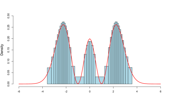
Figure 2: Example with $b(x)={\rm He}_{k}(x)^{2}/k!$ for $k=2$, $N=41$, where the breaks in the histogram are the successive $x_{n}$ satisfying the recursion (2.3) and the red curve is $p_{k}(x)$.

3 Generalized zero-bias transformations

Let $W$ be a symmetric random variable and $b\colon\mathbb{R}\to\mathbb{R}$ a non-negative function such that $\sigma^{2}=\mathbbm{E}[W^{2}/b(W)]<\infty$. Goldstein and Reinert (1997) gives a distributional fixed point characterization of the Gaussian distribution, which we generalize in the definition below.

Definition 3.1.

If there is a random variable $W^{\star}$ such that

$$\sigma^{2}\mathbbm{E}\left[\frac{f^{\prime}(W^{\star})}{b(W^{\star})}\right]=\mathbbm{E}\left[\frac{Wf(W)}{b(W)}\right]$$

for all absolutely continuous functions $f\colon\mathbb{R}\to\mathbb{R}$ such that $\mathbbm{E}|Wf(W)/b(W)|<\infty$, we say that $W^{\star}$ has the $b$-generalized-zero-bias distribution of $W$.

Remark 3.2.

Goldstein and Reinert (1997) study the case $b(x)=1$ and show that $W^{\star}$ has the same distribution as $W$ if and only if $W$ has a Gaussian distribution. Distributional fixed point characterizations for exponential, gamma and other nonnegative distributions and the connection with Stein’s method have been studied in Peköz and Röllin (2011), Peköz et al. (2013), and Peköz et al. (2016).

Remark 3.3.

By a routine extension of the proof of Proposition 2.1 of Chen et al. (2010), it can be shown that there exists a unique distribution for $W^{\star}$, and it is absolutely continuous with density

$$p^{\star}(x)\propto{b(x)}\mathbbm{E}\left[\frac{W}{b(W)}1_{W\geqslant x}\right].$$

We note in passing that the $\sigma^{2}$ is misplaced in the first display of Chen et al.’s proposition, which corresponds to $b(x)=1$, the usual zero-bias distribution of $W$. The composition of the $b$-generalized-zero-bias transformation with the $(1/b)$-generalized-zero-bias transformation is the usual zero-bias transformation.

Remark 3.4.

With $\varphi$ the standard normal density and $b$ a $\varphi$-integrable function, if $W$ has density

$$p(x)=b(x)\varphi(x),$$ (3.1)

then its distribution is a fixed point for the $b$-generalized-zero-bias transformation since

$$p^{\star}(x)=b(x)\int_{x}^{\infty}\frac{t}{b(t)}p(t)\,dt=b(x)\int_{x}^{\infty}t\varphi(t)\,dt=p(x).$$

The following result gives the $b$-generalized-zero-bias distribution of the uniform distribution on $N$ points.

Proposition 3.5.

Given an integer $N>1$, let $x_{1}>x_{2}>\ldots>x_{N}$ be such that $b(x_{n})>0$ for all $n$. Let $\mathbb{P}_{N}$ be the empirical distribution of the $x_{n}$:

$$\mathbb{P}_{N}(A)={\#\{n\colon x_{n}\in A\}\over N}$$

for any Borel set $A\subset\mathbb{R}$. Under the symmetry condition $x_{n}=x_{N-n+1}$ for $n=1,\ldots,N$, the $b$-generalized-zero-bias distribution ${\mathbb{P}}^{\star}_{N}$ of $\mathbb{P}_{N}$ is defined, and has density

$$p^{\star}(x)\propto b(x)\left[\sum_{i=1}^{n}\frac{x_{i}}{b(x_{i})}\right]$$

for $x_{n+1}<x\leq x_{n}$ ($n=1,\ldots,N-1$), and $p^{\star}(x)=0$ if $x>x_{1}$ or $x\leq x_{N}$.

Proof.

Immediate from Remark 3.3. ∎

Recall the following distances between distribution functions $F$ and $G$. The Kolmogorov distance is

$$\mathop{d_{\mathrm{K}}}(F,G)=\sup_{x\in\mathbbm{R}}|F(x)-G(x)|,$$

and the Wasserstein distance is

$$\mathop{d_{\mathrm{W}}}(F,G)=\sup_{h\in\mathcal{H}}\left|\int_{\mathbbm{R}}h\,dF-\int_{\mathbbm{R}}h\,dG\right|$$

where

$$\mathcal{H}=\{h\colon\mathbbm{R}\rightarrow\mathbbm{R}\mbox{ Lipschitz with }\|h^{\prime}\|\leqslant 1\}$$

and $\|\cdot\|$ is the supremum norm. Using Proposition 1.2 in Ross (2011), these two metrics are seen to be related by

$$\mathop{d_{\mathrm{K}}}(F,G)\leqslant\sqrt{2C\mathop{d_{\mathrm{W}}}(F,G)}$$

if $G$ has density bounded by $C$.

Restricting attention to the special case $b(x)=x^{2}$, we can now state our main result, along with an important corollary.

Theorem 3.6.

Suppose $W^{\star}$ is constructed on the same probability space as the zero-mean random variable $W$ and is distributed according to the $x^{2}$-generalized-zero-bias distribution of $W$. Let $M$ have the two-sided Maxwell density $x^{2}e^{-x^{2}/2}/\sqrt{2\pi}$. Then there exist positive finite constants $\lambda_{1},\lambda_{2},\lambda_{3}$ and $\lambda_{4}$ such that

$$\mathop{d_{\mathrm{W}}}(\mathscr{L}(W),\mathscr{L}(M)) \leq\lambda_{1}\mathbb{E}\left|W-W^{\star}\right|+\lambda_{2}\mathbb{E}\left[|W|\left|W-W^{\star}\right|\right]$$

$$\qquad\quad+\lambda_{3}\mathbb{E}\left|\frac{1}{W}-\frac{1}{W^{\star}}\right|+\lambda_{4}\mathbb{E}\left|1-\frac{W^{\star}}{W}\right|.$$ (3.2)

Proof.

The inequality follows immediately from Theorem 4.4. Finiteness of the constants (along with explicit upper bounds) is detailed in Proposition 4.5. ∎

The following corollary gives a rate of convergence of the solution to (1.4) to the two-sided Maxwell distribution in terms of the Wasserstein distance; we postpone the proof until Section 4.3.

Corollary 3.7.

Suppose $x_{1},\ldots x_{N}$ is a monotonic, zero-mean, finite sequence of real numbers satisfying (1.4), let $\mathbb{P}_{N}$ be the empirical distribution of these values, and let $M$ be as in Theorem 3.6. Then there is a constant $c>0$ such that

$$\mathop{d_{\mathrm{W}}}(\mathbb{P}_{N},\mathscr{L}(M))\leq c\sqrt{\frac{\log N}{N}}.$$

4 The Stein equation and its solutions

4.1 General considerations

Let $X$ have a density $p$ defined as in (3.1). The first step is to identify an appropriate “Stein equation” and bound its solutions. Let $\tilde{h}$ be such that $\mathbbm{E}[\tilde{h}(X)]=0$. There are many possible starting points. The well known “density approach” (see Chatterjee and Shao (2011)) starts with the Stein equation

$$f^{\prime}(x)+\frac{p^{\prime}(x)}{p(x)}f(x)=\tilde{h}(x)$$

which is easily solved to yield

$$f(x)=\frac{1}{b(x)\varphi(x)}\int_{x}^{\infty}\tilde{h}(u)b(u)\varphi(u)\,du.$$

If $b$ vanishes at a point, as it does in the two-sided Maxwell case where $b(0)=0$, then this solution $f$ will have a singularity and we cannot carry on with the usual program for applying Stein’s method. For these types of distributions we propose a new approach; the price we pay here is the necessity to bound several additional quantities concerning the couplings we obtain. The explicit nature of the recursion here allows us to compute these quantities.

In view of Definition 3.1 it is natural to consider the Stein equation

$$\frac{f^{\prime}(w)}{b(w)}-w\frac{f(w)}{b(w)}=\tilde{h}(w)$$ (4.1)

which can be solved using the usual normal approximation solution, but the resulting estimates will again rest on properties of $f/b$ which is unbounded in the cases we are interested in. Because of this, we introduce an original route which leads to the correct order bounds we are seeking.

First, following Ley, Reinert and Swan (2016) we introduce an integral operator associated with the Gaussian density:

$$\tilde{h}\mapsto\mathcal{T}_{\varphi}^{-1}\tilde{h}(w):=\frac{1}{\varphi(w)}\int_{w}^{\infty}\tilde{h}(u)\varphi(u)\,du$$ (4.2)

(called the “inverse Stein operator”) mapping functions with Gaussian-mean zero and sufficiently well-behaved tails into bounded functions. Next define the “Stein kernel” of $X$ (or, equivalently, of $p$) by

$$\tau_{X}(x)=\frac{1}{p(x)}\int_{x}^{\infty}up(u)\,du.$$

The Stein kernel satisfies the integration by parts formula

$$\mathbbm{E}\left[\tau_{X}(X)f^{\prime}(X)\right]=\mathbbm{E}\left[Xf(X)\right]$$ (4.3)

for all sufficiently regular functions $f$. Stein kernels were introduced in Stein (1986), Cacoullos and Papathanasiou (1989), and have proven to be of great use in Gaussian analysis, see, e.g., Nourdin and Peccati (2009) and Chatterjee (2009).

Remark 4.1.

As discussed in the Introduction, our concern in this paper is with symmetric densities of the form $p_{k}(x)$ given in (1.2). The Stein kernel of $p_{k}$ is

$$\tau_{k}(x)=\int_{x}^{\infty}u{\rm He}_{k}(u)^{2}\varphi(u)\,du/(\varphi(x){\rm He}_{k}(x)^{2})$$

and direct integration leads to

$$\tau_{1}(x)=\frac{x^{2}+2}{x^{2}},\ \tau_{2}(x)=\frac{x^{4}+2x^{2}+5}{(x^{2}-1)^{2}},\ \tau_{3}(x)=\frac{x^{6}+9x^{2}+18}{(x^{3}-3x)^{2}}.$$ (4.4)

The next result applies to general densities, but in the following sections we focus on further results for the special case $\tau_{1}(x).$

We aim to assess the proximity between the law of $X$ and some $W$ by estimating the Wasserstein distance between their distributions. Suppose that there exists a $W^{\star}$ following the $b$-generalized-zero-bias distribution of $W$ and defined on the same probability space as $W$. To each integrable test function $h$ we associate the function $f:=f_{h}$, the solution to (4.1) with $\tilde{h}=h-\mathbbm{E}h(X)$. This association is unique in the sense that there exists only one absolutely continuous version of $f$ satisfying (4.1) at all points $x$, see e.g. Chen et al. (2010). We then write (supposing here and in the sequel that $\sigma^{2}=1$)

$$\mathbbm{E}\left[h(W)\right]-\mathbbm{E}\left[h(X)\right]=\mathbbm{E}\left[\frac{f^{\prime}(W)}{b(W)}-W\frac{f(W)}{b(W)}\right]$$

$$=\mathbbm{E}\left[\frac{f^{\prime}(W)}{b(W)}-\frac{f^{\prime}(W^{\star})}{b(W^{\star})}\right].$$ (4.5)

One of the major differences between the present setting and the usual applications of Stein’s method is that here we cannot bound the right hand side of (4.5) directly because solutions $f$ of (4.1) have a singularity at 0. In order to bypass this difficulty it was therefore necessary to introduce some further tweaking of the method which we now detail. Such results should also have an intrinsic interest for users of Stein’s method as it bears natural generalizations for density functions of the form $p(x)=b(x)p_{0}(x)$ with $p_{0}$ and $b$ well chosen.

Proposition 4.2.

Let $x\mapsto b(x)$ be a nonnegative even function with support in $(-\infty,\infty)$ such that $\lim_{x\to\pm\infty}b(x)\varphi(x)=0$. Suppose furthermore that $b$ is absolutely continuous and integrable w.r.t. $\varphi$ with integral $\int_{-\infty}^{\infty}b(x)\varphi(x)\,dx=1$. Let $X$ be a random variable with density $x\mapsto b(x)\varphi(x)$. Then

$$\tau_{X}(x)=1+\frac{\mathcal{T}_{\varphi}^{-1}b^{\prime}(x)}{b(x)}$$ (4.6)

under the convention that the ratio is set to zero at all points $x$ such that $b(x)=0$ and $\mathcal{T}_{\varphi}^{-1}b^{\prime}(x)\neq 0$. Further, with $\tilde{h}$ defined by (4.1),

$$g_{h}(x)=\frac{{\int_{x}^{\infty}b(u)\tilde{h}(u)\varphi(u)\,du}}{{b(x)\varphi(x)+\int_{x}^{\infty}b^{\prime}(u)\varphi(u)\,du}}$$ (4.7)

is the unique bounded solution of the ODE

$$\tau_{X}(x)g^{\prime}(x)-xg(x)=\tilde{h}.$$ (4.8)

Proof.

Integrating by parts in the definition of the Stein kernel for $p=b\varphi$ we get (assuming that $\lim_{x\to\pm\infty}b(x)\varphi(x)=0$)

$$\int_{x}^{+\infty}yp(y)\,dy =\int_{x}^{\infty}b(y)(-\varphi^{\prime}(y))\,dy$$

$$=b(x)\varphi(x)+\int_{x}^{\infty}b^{\prime}(y)\varphi(y)dy$$

so that (4.6) follows by definition (4.2) of the inverse Stein operator. For the second claim note how

$$\tau_{X}(x)g^{\prime}(x)-xg(x)=\frac{\left(\tau_{X}(x)g(x)p(x)\right)^{\prime}}{p(x)}$$

so that the conclusion (along with unicity) follows from the same argument as in (Nourdin and Peccati, 2012, Proposition 3.2.2) ∎

Intuition (supported e.g. by (Stein, 1986, Lesson VI) or the more recent work Döbler (2015)) encourages us to claim that functions (4.7) will have satisfactory behavior. It is thus natural to seek a connection between equations of the form (4.1) and (4.8). This we summarize in the next lemma.

Lemma 4.3.

Let all notations be as above and introduce the function $g=g_{f}$ defined at all $x$ through

$$\frac{f^{\prime}(x)-xf(x)}{b(x)}=\tau_{X}(x)g^{\prime}(x)-xg(x).$$

Then

$$\mathbbm{E}\left[\frac{f^{\prime}(W)}{b(W)}-\frac{f^{\prime}(W^{\star})}{b(W^{\star})}\right] =\mathbbm{E}\left[W(\tau_{X}(W)-1)g(W)-W^{\star}(\tau_{X}(W^{\star})-1)g(W^{\star})\right]$$

$$\quad\quad+\mathbbm{E}\left[\tau_{X}(W)g^{\prime}(W)-\tau_{X}(W^{\star})g^{\prime}(W^{\star})\right].$$ (4.9)

Proof.

Since

$$\frac{f^{\prime}(x)-xf(x)}{b(x)}=\frac{(f(x)\varphi(x))^{\prime}}{b(x)\varphi(x)}$$

and

$$\tau_{X}(x)g^{\prime}(x)-xg(x)=\frac{(b(x)\tau_{X}(x)g(x)\varphi(x))^{\prime}}{b(x)\varphi(x)}$$

at all $x$ for which $b(x)\neq 0$, we deduce that $f$ and $g$ are mutually defined by $f=(b\tau_{X})g$. This in turn gives

$$\frac{f^{\prime}(x)}{b(x)}=\left(\frac{b^{\prime}(x)}{b(x)}\tau_{X}(x)+\tau_{X}^{\prime}(x)\right)g(x)+\tau_{X}(x)g^{\prime}(x)=:\psi(x)g(x)+\tau_{X}(x)g^{\prime}(x)$$

which, combined with $\psi(x)=x(\tau_{X}(x)-1)$ (that is easily derived using the various definitions involved), leads to the useful identity

$$\frac{f^{\prime}(x)}{b(x)}=x(\tau_{X}(x)-1)g(x)+\tau_{X}(x)g^{\prime}(x)$$ (4.10)

from which (4.9) is directly derived. ∎

In view of Lemma 4.3 and identity (4.5) it remains to find bounds on the two terms on the right hand side of (4.9).

4.2 Approximating the two-sided Maxwell distribution

Theorem 4.4.

Let $p(x)=x^{2}\varphi(x)$, and take $f$ a solution to the Stein equation

$$f^{\prime}(w)/w^{2}-wf(w)/w^{2}=\tilde{h}(w),$$ (4.11)

where $\tilde{h}$ is a function having bounded first derivative and zero-mean under $p$. Set $c=\|\tilde{h}^{\prime}\|$. Then for any coupling of $W$ and $W^{*}$ on a joint probability space such that $W^{*}$ has the $x^{2}$-generalized zero biased distribution for $W$,

$$\left|\mathbb{E}\left[\frac{f^{\prime}(W)}{(W)^{2}}-\frac{f^{\prime}(W^{\star})}{(W^{\star})^{2}}\right]\right| \leq\lambda_{1}\mathbb{E}\left|W-W^{\star}\right|+\lambda_{2}\mathbb{E}\left[|W|\left|W-W^{\star}\right|\right]$$

$$\qquad\quad+\lambda_{3}\mathbb{E}\left|\frac{1}{W}-\frac{1}{W^{\star}}\right|+\lambda_{4}\mathbb{E}\left|1-\frac{W^{\star}}{W}\right|$$ (4.12)

with

$$\lambda_{1}\leq 6c,\,\lambda_{2}\leq 7c,\,\lambda_{3}\leq 18c\mbox{ and }\lambda_{4}\leq 22c.$$ (4.13)

Proof.

With $b(x)=x^{2}$ we have $\tau_{X}(x)=1+2/x^{2}$ and $\psi(x)=2/x$, so that (4.9) becomes

$$=\mathbb{E}\left[\frac{2}{W^{\star}}g(W^{\star})-\frac{2}{W}g(W)\right]+\mathbb{E}\left[\left(1+\frac{2}{(W^{\star})^{2}}\right)g^{\prime}(W^{\star})-{\left(1+\frac{2}{(W)^{2}}\right)}g^{\prime}(W)\right]$$

$$=2\mathbb{E}\left[\left(\frac{1}{W^{\star}}-\frac{1}{W}\right)g(W^{\star})\right]+2\mathbb{E}\left[\frac{1}{W}\left(g(W^{\star})-g(W)\right)\right]$$

$$\quad+\mathbb{E}\left[g^{\prime}(W^{\star})-g^{\prime}(W)\right]+2\mathbb{E}\left[\frac{1}{(W^{\star})^{2}}g^{\prime}(W^{\star})-\frac{1}{(W)^{2}}g^{\prime}(W)\right].$$

The first two terms are dealt with easily to get

$$2\left|\mathbb{E}\left[\left(\frac{1}{W^{\star}}-\frac{1}{W}\right)g(W^{\star})\right]+2\mathbb{E}\left[\frac{1}{W}\left(g(W^{\star})-g(W)\right)\right]\right|$$

$$\leq 2\|g\|\mathbb{E}\left[\left|\frac{1}{W^{\star}}-\frac{1}{W}\right|\right]+2\|g^{\prime}\|\mathbb{E}\left[\frac{1}{|W|}\left|W^{\star}-W\right|\right].$$

For the last two terms we introduce the function

$$\chi(x)=g^{\prime}(x)/x$$

to get on the one hand

$$\mathbb{E}\left[g^{\prime}(W^{\star})-g^{\prime}(W)\right] =\mathbb{E}\left[W^{\star}\frac{g^{\prime}(W^{\star})}{W^{\star}}-W\frac{g^{\prime}(W)}{W}\right]$$

$$=\mathbb{E}\left[(W^{\star}-W)\chi(W^{\star})\right]+\mathbb{E}\left[W\left(\chi(W^{\star})-\chi(W)\right)\right]$$

so that

$$\left|\mathbb{E}\left[g^{\prime}(W^{\star})-g^{\prime}(W)\right]\right|\leq\|\chi\|E\left[\left|W^{\star}-W\right|\right]+\|\chi^{\prime}\|E\left[\left|W(W^{\star}-W)\right|\right]$$

and, on the other hand

$$\mathbb{E}\left[\frac{1}{(W^{\star})^{2}}g^{\prime}(W^{\star})-\frac{1}{(W)^{2}}g^{\prime}(W)\right] =\mathbb{E}\left[\frac{1}{W^{\star}}\chi(W^{\star})-\frac{1}{W}\chi(W)\right]$$

$$=\mathbb{E}\left[\left(\frac{1}{W^{\star}}-\frac{1}{W}\right)\chi(W^{\star})\right]+\mathbb{E}\left[\frac{1}{W}\left(\chi(W^{\star})-\chi(W)\right)\right]$$

so that

$$2\left|\mathbb{E}\left[\frac{1}{(W^{\star})^{2}}g^{\prime}(W^{\star})-\frac{1}{(W)^{2}}g^{\prime}(W)\right]\right|\leq 2\|\chi\|\mathbb{E}\left[\left|\frac{1}{W^{\star}}-\frac{1}{W}\right|\right]+2\|\chi^{\prime}\|\mathbb{E}\left[\frac{1}{|W|}\left|W^{\star}-W\right|\right].$$

Combining these different estimates we obtain (4.12), with $\lambda_{1},\lambda_{2},\lambda_{3}$ and $\lambda_{4}$ expressed in terms of $\|\chi\|,\|\chi^{\prime}\|,\|g\|$ and $\|g^{\prime}\|$ as follows:

$$\lambda_{1}=\|\chi\|,\lambda_{2}=\|\chi^{\prime}\|,\lambda_{3}=2(\|g\|+\|\chi\|)\mbox{ and }\lambda_{4}=2(\|g^{\prime}\|+\|\chi^{\prime}\|).$$

The inequalities in (4.13) are proved in the Proposition 4.5 below. ∎

The next step is to bound $\|\chi\|,\|\chi^{\prime}\|,\|g\|$ and $\|g^{\prime}\|$ in a non trivial way; this we achieve in the next proposition.

Proposition 4.5.

Let $h:\mathbb{R}\to\mathbb{R}$ be absolutely continuous and integrable with respect to $p(x)=x^{2}\varphi(x)$. Set $c=\|h^{\prime}\|$ which we suppose to be finite. Let $X\sim p$, define

$$g_{0}(x)=\left\{\begin{array}[]{cl}e^{x^{2}/2}\int_{x}^{\infty}y^{2}\left(h(y)-\mathbbm{E}\left[h(X)\right]\right)e^{-y^{2}/2}\,dy&\mbox{ if }x>0\\ e^{x^{2}/2}\int_{-\infty}^{x}y^{2}\left(h(y)-E\left[h(X)\right]\right)e^{-y^{2}/2}\,dy&\mbox{ if }x\leq 0\\ \end{array}\right.$$ (4.16)

and set

$$g(x)=\frac{g_{0}(x)}{x^{2}+2}\mbox{ and }\chi(x)=\frac{g^{\prime}(x)}{x}.$$ (4.17)

Then

$$\|g\|\leq 3c,\|g^{\prime}\|\leq 4c,\|\chi\|\leq 6c\mbox{ and }\|\chi^{\prime}\|\leq 7c.$$

Remark 4.6.

The function $g_{0}$ defined in (4.16) satisfies

$$g_{0}^{\prime}(x)-xg_{0}(x)=x^{2}\left(h(x)-\mathbbm{E}[Z^{2}h(Z)]\right)$$ (4.18)

with $Z\sim\varphi$ a standard Gaussian random variable.

Remark 4.7.

The function $g$ defined in (4.17) satisfies

$$\frac{\left(g(x)\tau(x)p(x)\right)^{\prime}}{p(x)}=h(x)-\mathbbm{E}\left[h(X)\right]$$

with $X\sim p$ and $\tau(x)=1+2/x^{2}$.

Proof.

In order to simplify future notations we introduce $\Phi(x)=\int_{-\infty}^{x}\varphi(t)\,dt,$ $\bar{\Phi}(x)=\int_{x}^{\infty}\varphi(t)\,dt$ $\Upsilon(x)=e^{x^{2}/2}\int_{x}^{\infty}t^{2}e^{-t^{2}/2}\,dt$ and $\bar{\Upsilon}(x)=e^{x^{2}/2}\int_{-\infty}^{x}t^{2}e^{-t^{2}/2}\,dt.$ Using the identity

$$\int_{a}^{b}t^{2}e^{-t^{2}/2}\,dt=ae^{-a^{2}/2}-be^{-b^{2}/2}+\int_{a}^{b}e^{-t^{2}/2}\,dt,\quad-\infty\leq a<b\leq\infty,$$ (4.19)

we deduce that $\Upsilon(x)=x+e^{x^{2}/2}\int_{x}^{\infty}e^{-t^{2}/2}\,dt$ and $\bar{\Upsilon}(x)=-x+e^{x^{2}/2}\int_{-\infty}^{x}e^{-t^{2}/2}\,dt$ and thus

$$\Upsilon(x),\bar{\Upsilon}(x)\leq|x|+\sqrt{\frac{\pi}{2}}\mbox{ at all }x\in\mathbb{R}\mbox{ and }\lim_{x\to\infty}\frac{\Upsilon(x)}{x}=\lim_{x\to-\infty}\frac{\bar{\Upsilon}(x)}{x}=1.$$ (4.20)

The proof is now broken down into several steps.

Step 1: rewrite the solutions. Following (Chen et al., 2010, page 39) we rewrite the test functions in term of their derivatives (still with $Z$ a standard normal random variable)

$$h(y)-E\left[h(X)\right]=h(y)-E\left[Z^{2}h(Z)\right]$$

$$=\int_{-\infty}^{\infty}z^{2}\left(h(y)-h(z)\right)\varphi(z)\,dz$$

$$=\int_{-\infty}^{y}z^{2}\left(\int_{z}^{y}h^{\prime}(t)\,dt\right)\varphi(z)\,dz-\int_{y}^{\infty}z^{2}\left(\int_{y}^{z}h^{\prime}(t)\,dt\right)\varphi(z)\,dz.$$

Changing the order of integration then using (4.19) leads to the rhs becoming

$$\int_{-\infty}^{y}h^{\prime}(t)\left[\int_{-\infty}^{t}z^{2}\varphi(z)\,dz\right]\,du-\int_{y}^{\infty}h^{\prime}(t)\left[\int_{t}^{\infty}z^{2}\varphi(z)\,dz\right]\,dt$$

$$=\int_{-\infty}^{y}h^{\prime}(t)\left[-t\varphi(t)+\int_{-\infty}^{t}\varphi(z)dz\right]\,dt-\int_{y}^{\infty}h^{\prime}(t)\left[t\varphi(t)+\int_{t}^{\infty}\varphi(z)\,dz\right]\,dt$$

$$=-\int_{-\infty}^{\infty}h^{\prime}(t)t\varphi(t)\,dt+\int_{-\infty}^{y}h^{\prime}(t)\Phi(t)\,dt-\int_{y}^{\infty}h^{\prime}(t)\bar{\Phi}(t)\,dt,$$

and thus

$$h(y)-E\left[h(X)\right]=\int_{-\infty}^{y}h^{\prime}(t)\Phi(t)dt-\int_{y}^{\infty}h^{\prime}(t)\bar{\Phi}(t))dt-E\left[Zh^{\prime}(Z)\right].$$ (4.21)

We deduce the following useful bound

$$\frac{h(x)-E\left[h(X)\right]}{x^{2}+2}\leq c\frac{2(x+1/\sqrt{2\pi})+\sqrt{2/\pi}}{x^{2}+2}\leq 2c.$$ (4.22)

Plugging (4.21) in (4.16) leads to (we restrict the discussion to $x>0$, the other case following by symmetry)

$$g_{0}(x) =-\mathbbm{E}[Zh^{\prime}(Z)]\Upsilon(x) =:I(x)$$

$$\quad+e^{x^{2}/2}\int_{x}^{\infty}\int_{-\infty}^{y}y^{2}e^{-y^{2}/2}h^{\prime}(t)\Phi(t)\,dtdy =:II(x)$$

$$\quad-e^{x^{2}/2}\int_{x}^{\infty}\int_{y}^{{\infty}}y^{2}e^{-y^{2}/2}h^{\prime}(t)\bar{\Phi}(t)\,dtdy =:III(x)$$

To deal with the quantities $II(x)$ and $III(x)$ we again interchange integrations to get

$$II(x) =e^{x^{2}/2}\int_{-\infty}^{x}\left(\int_{x}^{\infty}y^{2}e^{-y^{2}/2}\,dy\right)h^{\prime}(t)\Phi(t)\,dt$$

$$\quad+e^{x^{2}/2}\int_{x}^{\infty}\left(\int_{t}^{\infty}y^{2}e^{-y^{2}/2}\,dy\right)h^{\prime}(t)\Phi(t)\,dt$$

$$=\Upsilon(x)\int_{-\infty}^{x}h^{\prime}(t)\Phi(t)\,dt+e^{x^{2}/2}\int_{x}^{\infty}e^{-t^{2}/2}\Upsilon(t)h^{\prime}(t)\Phi(t)\,dt$$

and

$$III(x) =e^{x^{2}/2}\int_{x}^{\infty}\left(\int_{x}^{t}y^{2}e^{-y^{2}/2}\,dy\right)h^{\prime}(t)\bar{\Phi}(t)\,dt$$

$$=e^{x^{2}/2}\int_{x}^{\infty}\left(e^{-x^{2}/2}\Upsilon(x)-e^{-t^{2}/2}\Upsilon(t)\right)h^{\prime}(t)\bar{\Phi}(t)\,dt$$

$$=\Upsilon(x)\int_{x}^{\infty}h^{\prime}(t)\bar{\Phi}(t)\,dt-e^{x^{2}/2}\int_{x}^{\infty}e^{-t^{2}/2}\Upsilon(t)h^{\prime}(t)\bar{\Phi}(t)\,dt$$

and thus if $x\geq 0$ we have

$$g_{0}(x) =-\mathbbm{E}[Zh^{\prime}(Z)]\Upsilon(x)+\Upsilon(x)\int_{-\infty}^{x}h^{\prime}(t)\Phi(t)\,dt$$

$$\quad-\Upsilon(x)\int_{x}^{\infty}h^{\prime}(t)\bar{\Phi}(t)\,dt+e^{x^{2}/2}\int_{x}^{\infty}e^{-t^{2}/2}\Upsilon(t)h^{\prime}(t)\,dt.$$ (4.23)

By a similar argument we deduce that if $x<0$ then

$$g_{0}(x) =-\mathbbm{E}[Zh^{\prime}(Z)]\Upsilon(x)+\Upsilon(x)\int_{-\infty}^{x}h^{\prime}(t)\bar{\Phi}(t)\,dt$$

$$\quad-\Upsilon(x)\int_{x}^{\infty}h^{\prime}(t)\Phi(t)\,dt+e^{x^{2}/2}\int_{-\infty}^{x}e^{-t^{2}/2}\Upsilon(t)h^{\prime}(t)\,dt.$$ (4.24)

Step 2: a bound on $\|g\|$. Supposing $\|h^{\prime}\|\leq c$ we can use (4.2) and the first claim in (4.20) to deduce that for $x\geq 0$:

$$\left|g_{0}(x)\right| \leq cE\left|Z\right|(x+\sqrt{\pi/2})+c(x+\sqrt{\pi/2})\int_{-\infty}^{x}\Phi(t)\,dt$$

$$\quad+c(x+\sqrt{\pi/2})\int_{x}^{\infty}\bar{\Phi}(t)\,dt+ce^{x^{2}/2}\int_{x}^{\infty}e^{-t^{2}/2}(t+\sqrt{\pi/2})\,dt.$$

The last two terms decrease strictly to 0 as $x\to\infty$, with maximum value $c/2$ and $c(1+\pi/2)$, respectively. The first term is equal to $c(\sqrt{2/\pi}x+1)$ and the second one is equal to

$$c(x+\sqrt{\pi/2})\int_{-\infty}^{x}\Phi(t)\,dt =c(x+\sqrt{\pi/2})\left(x\Phi(x)+\varphi(x)\right)$$

$$\leq c(x^{2}+(\sqrt{\pi/2}+1/\sqrt{2\pi})x+1/2).$$

Similar (symmetric) bounds hold for $x\leq 0$ and thus, collecting all these estimates, we may conclude:

$$|g(x)|=\frac{|g_{0}(x)|}{x^{2}+2}\leq 3c.$$ (4.25)

Step 3: a bound on $\|g^{\prime}\|$. Here we start by rewriting the derivative as

$$g^{\prime}(x)=\frac{g_{0}^{\prime}(x)}{x^{2}+2}-\frac{2x}{(x^{2}+2)^{2}}g_{0}(x).$$ (4.26)

Using (4.25), the second summand is easily seen to be uniformly bounded (by $3c$). We are left with the first summand for which we start by rewriting the numerator, for $x\geq 0$, using (4.2):

$$g_{0}^{\prime}(x) =-\Upsilon^{\prime}(x)\mathbbm{E}[Zh^{\prime}(Z)]+\Upsilon^{\prime}(x)\int_{-\infty}^{x}h^{\prime}(t){\Phi}(t)\,dt$$

$$\quad-\Upsilon^{\prime}(x)\int_{x}^{\infty}h^{\prime}(t)\bar{\Phi}(t)\,dt$$

$$\quad+\Upsilon(x)\left(h^{\prime}(x){\Phi}(x)+h^{\prime}(x)\bar{\Phi}(x)\right)$$

$$\quad+xe^{x^{2}/2}\int_{x}^{\infty}\Upsilon(t)h^{\prime}(t)e^{-t^{2}/2}\,dt-e^{x^{2}/2}\Upsilon(x)h^{\prime}(x)e^{-x^{2}/2}$$

which leads to

$$g_{0}^{\prime}(x) =-\Upsilon^{\prime}(x)\mathbbm{E}[Zh^{\prime}(Z)]$$

$$\quad+\Upsilon^{\prime}(x)\int_{-\infty}^{x}h^{\prime}(t){\Phi}(t)\,dt-\Upsilon^{\prime}(x)\int_{x}^{\infty}h^{\prime}(t)\bar{\Phi}(t)\,dt$$

$$\quad+xe^{x^{2}/2}\int_{x}^{\infty}\Upsilon(t)h^{\prime}(t)e^{-t^{2}/2}\,dt.$$ (4.27)

Now we can use the fact that $\Upsilon^{\prime}(x)=xe^{x^{2}/2}\int_{x}^{\infty}e^{-t^{2}/2}\,dt\leq 1\mbox{ for all }x\geq 0$ as well as all the arguments outlined at the previous step to deduce the bound: $|g_{0}^{\prime}(x)|\leq c\left(\sqrt{\frac{2}{\pi}}+2(x+1/\sqrt{2\pi})+\frac{1}{\sqrt{2\pi}}\right)\leq 2c(x+1)$ whence

$$\frac{|g_{0}^{\prime}(x)|}{x^{2}+2}\leq c\frac{2x+2}{x^{2}+2}\leq c.$$ (4.28)

Similar (symmetric) arguments hold also for negative $x$ and thus $|g^{\prime}(x)|\leq 4c.$

Step 4: a bound on $\chi(x)=g^{\prime}(x)/x$. Using (4.26) we know that

$$\chi(x) =\frac{g_{0}^{\prime}(x)}{x(x^{2}+2)}-\frac{1}{(x^{2}+2)^{2}}g_{0}(x).$$ (4.29)

The second summand in (4.29) is bounded using (4.2) to get

$$\frac{1}{(x^{2}+2)^{2}}\left|g_{0}(x)\right|\leq 3c.$$ (4.30)

For the first summand we use (4.27) to deduce

$$\frac{g_{0}^{\prime}(x)}{x} =-\frac{\Upsilon^{\prime}(x)}{x}\mathbbm{E}[Zh^{\prime}(Z)]$$

$$\quad+\frac{\Upsilon^{\prime}(x)}{x}\int_{-\infty}^{x}h^{\prime}(t){\Phi}(t)\,dt-\frac{\Upsilon^{\prime}(x)}{x}\int_{x}^{\infty}h^{\prime}(t)\bar{\Phi}(t)\,dt$$

$$\quad+e^{x^{2}/2}\int_{x}^{\infty}\Upsilon(t)h^{\prime}(t)e^{-t^{2}/2}\,dt.$$

At this stage it is useful to remark that, for $x\geq 0$, the function ${\Upsilon^{\prime}(x)}/{x}$ is strictly decreasing with maximal value $\sqrt{\pi/2}$ and hence $\left|\frac{g_{0}^{\prime}(x)}{x}\right|\leq c\left(1+2\left(x+\frac{1}{\sqrt{2\pi}}\right)+\frac{1}{\sqrt{2\pi}}\right)\leq c\left(2x+3\right)$ and thus $\left|\frac{g_{0}^{\prime}(x)}{x(x^{2}+2)}\right|\leq 3c$ which, combined with (4.30), leads (after applying the symmetric arguments for $x\leq 0$) to $\left|\chi(x)\right|\leq 6c.$

Step 5: a bound on $\|\chi^{\prime}\|$. Direct computations using (4.18)

$$\chi(x)=\frac{1}{x^{2}+2}\left(1-\frac{1}{x^{2}+2}\right)g_{0}(x)-\frac{x}{x^{2}+2}\left(h(x)-\mathbbm{E}[Z^{2}h(Z)]\right)$$

and thus

$$\chi^{\prime}(x) =-\frac{2x^{3}}{(x^{2}+2)^{2}}\frac{g_{0}(x)}{x^{2}+2}+\left(1-\frac{2}{x^{2}+2}\right)\frac{g_{0}^{\prime}(x)}{x^{2}+2}$$

$$\qquad-\frac{2-x^{2}}{x^{2}+2}\frac{h(x)-\mathbbm{E}[Z^{2}h(Z)]}{x^{2}+2}-\frac{x}{x^{2}+2}h^{\prime}(x).$$

Using the bounds $\left|{2x^{3}}/{(x^{2}+2)^{2}}\right|\leq 1,$ $\left|1-{2}/({x^{2}+2})\right|\leq 1,$ $\left|({2-x^{2}})/({x^{2}+2})\right|\leq 1$ and $\left|{x}/({x^{2}+2})\right|\leq 1$ as well as (4.25), (4.28) and (4.22) we conclude (after applying the symmetric arguments for $x\leq 0$) $\left|\chi^{\prime}(x)\right|\leq 7c.$

∎

4.3 Verifying bounds on expectations

In this section we find bounds on the expectations in Theorem 3.6 in order to prove Corollary 3.7. We will make use of the following lemma.

Lemma 4.8.

If $x_{1},\ldots,x_{N}$ is the unique strictly decreasing zero-mean solution of (1.4), then $x_{1}=O(\sqrt{\log N})$.

Proof.

To simplify the notation, note that it suffices to consider the rescaled recursion $x_{n+1}^{3}=x_{n}^{3}-S_{n}^{-1}$, where $S_{n}$ is defined in the proof of Lemma 2.1. By expressing $x_{1}^{3}$ as a telescoping sum,

$$x_{1}^{3}=\sum_{n=1}^{m-1}(x_{n}^{3}-x_{n+1}^{3})+x_{m}^{3}=\sum_{n=1}^{m-1}S_{n}^{-1}+x_{m}^{3}\leq\sum_{n=1}^{m-1}(n/x_{1})^{-1}+x_{m}^{3}\leq x_{1}(1+\log m)+x_{m}^{3},$$

where we have used Euler’s approximation to the harmonic sum for the last inequality. By the variance property (P2) (in this rescaled case $x_{1}^{2}+\ldots+x_{N}^{2}=N-1$) we have that $x_{1}$ is bounded away from zero (as a sequence indexed by $N$) and $x_{m}$ is bounded, so $x_{m}^{2}/x_{1}$ is bounded. Dividing the above display by $x_{1}$, we then obtain $x_{1}=O(\sqrt{\log N})$.∎

Proof of Corollary 3.7.

From Proposition 3.5 and the recursion (1.4), note that $p^{\star}(x)$ puts mass $1/(N-1)$ on each interval between successive $x_{n}$, so it is easy to create a coupling of $W\sim\mathbb{P}_{N}$ with $W^{\star}\sim p^{\star}(x)$ such that

$$|W-W^{\star}|\leq|x_{n}-x_{n+1}|$$

when $W\in[x_{n+1},x_{n}]$. For a detailed proof of such a coupling, see the construction given in McKeague and Levin (2016). From Lemma 4.8 we then have

$$\mathbbm{E}|W-W^{\star}|\leq{1\over N-1}\sum_{n=1}^{N-1}(x_{n}-x_{n+1})={2x_{1}\over N-1}=O\left(\frac{\sqrt{\log N}}{N}\right).$$ (4.31)

Second, using $|W|\leq x_{1}=O(\sqrt{\log N})$ it follows immediately that

$$\mathbbm{E}[|W||W-W^{\star}|]=O\left(\frac{{\log N}}{N}\right).$$

Third, the zero-median property gives

$$2x_{m}^{3}=x_{m}^{3}-x_{m+1}^{3}={S_{m}^{-1}}\geq(m/x_{m})^{-1}={x_{m}}/{m},$$

where $m=N/2+1$, so $x_{m}\geq 1/\sqrt{N}$. By symmetry

$$\mathbbm{E}\left|\frac{1}{W}-\frac{1}{W^{\star}}\right|=\mathbbm{E}\left|\frac{1}{W}-\frac{1}{W^{\star}}\right|1_{W^{\star}\in(x_{m+1},x_{m}]}+2\sum_{n=1}^{m-1}\mathbbm{E}\left|\frac{1}{W}-\frac{1}{W^{\star}}\right|1_{W^{\star}\in(x_{n+1},x_{n}]}.$$

From Proposition 3.5 note that $p^{\star}(x)\propto x^{2}$ for $x\in(x_{m+1},x_{m}]$. Also using the fact that $p^{\star}(x)$ puts mass $1/(N-1)$ on this interval, the first term above can be written

$$\frac{6}{x_{m}^{3}(N-1)}\int_{0}^{x_{m}}\left({1\over x}-{1\over x_{m}}\right)x^{2}\,dx\leq\frac{3}{x_{m}(N-1)}=O\left({\frac{1}{\sqrt{N}}}\right).$$

The second term is bounded above by the telescoping sum

$${2\over N-1}\sum_{n=1}^{m-1}\left({1\over x_{n+1}}-{1\over x_{n}}\right)={2\over N-1}\left({1\over x_{m}}-{1\over x_{1}}\right)=O\left({\frac{1}{\sqrt{N}}}\right),$$

so we have

$$\mathbbm{E}\left|\frac{1}{W}-\frac{1}{W^{\star}}\right|=O\left({\frac{1}{\sqrt{N}}}\right).$$

Fourth,

$$\mathbbm{E}\left|1-\frac{W^{\star}}{W}\right|\leq\sqrt{N}\,\mathbbm{E}|W-W^{\star}|=O\left(\sqrt{\frac{\log N}{N}}\right)$$

using $|W|\geq x_{m}\geq 1/\sqrt{N}$ and (4.31). The Corollary now follows from Theorem 3.6. ∎

References

• Bohm (1952) D. Bohm (1952). A suggested interpretation of the quantum theory in terms of “hidden” variables. I. Phys. Rev. 85, 166–179.
• Cacoullos and Papathanasiou (1989) T. Cacoullos and V. Papathanasiou (1989). Characterizations of distributions by variance bounds. Statist. Probab. Lett. 7, 351–356.
• Chatterjee (2009) S. Chatterjee (2009). Fluctuations of eigenvalues and second order Poincaré inequalities. Probab. Theory Related Fields 143 1–40.
• Chatterjee and Shao (2011) S. Chatterjee and Q.-M. Shao (2011). Non-normal approximation by Stein’s method of exchangeable pairs with application to the Curie–Weiss model. Ann. App. Probab. 21, 464–483.
• Chen et al. (2010) L. Chen, L. Goldstein and Q.-M. Shao (2010). Normal Approximation by Stein’s Method. Springer Verlag.
• Döbler (2015) C. Döbler (2015). Stein’s method of exchangeable pairs for the beta distribution and generalizations. Electron. J. Probab. 20, 1–34.