Speciation in the Derrida-Higgs model with finite genomes and spatial populations

Abstract

The speciation model proposed by Derrida and Higgs demonstrated that a sexually reproducing population can split into different species in the absence of natural selection or any type of geographic isolation, provided that mating is assortative and the number of genes involved in the process is infinite. Here we revisit this model and simulate it for finite genomes, focusing on the question of how many genes it actually takes to trigger neutral sympatric speciation. We find that, for typical parameters used in the original model, it takes of the order of $10^{5}$ genes. We compare the results with a similar spatially explicit model where about 100 genes suffice for speciation. We show that when the number of genes is small the species that emerge are strongly segregated in space. For larger number of genes, on the other hand, the spatial structure of the population is less important and the species distribution overlap considerably.

I Introduction

Speciation requires the evolution of reproductive isolation between initially compatible individuals mayr_1942 . One of the most accepted mechanisms for the development of reproductive barriers is the geographic isolation of the populations, which can be complete (allopatry) or partial (parapatry) coyne_speciation_2004 ; nostil_2012 . In both cases the reduction of gene flow between individuals inhabiting different regions facilitates the fixation of local adaptations. These, in turn, may lead to pre-zygotic or post-zygotic mating incompatibilities and can eventually develop into full reproductive isolation.

Sympatric speciation, where new species arise from a population inhabiting a single geographic region, has been highly debated kirk-2004 ; Bolnick_2007 and its occurrence in nature is documented in only a few cases kondra-1986 ; coyne_speciation_2004 . Mathematical models have shown that sympatric speciation is theoretically possible Udovic_1980 ; Felsenstein_1981 ; kondra-1998 ; kondra-1999 ; Doebeli_2005 ; Gavrilets_2006 and the model by Dieckmann and Doebeli Dieckmann_1999 , in particular, attracted a lot of attention. In their model, speciation results from the interplay between strong competition for resources and the way resources are distributed. It was shown that, under appropriate conditions, the population will evolve in such a way as to consume the most abundant type of resource, but it will arrive at the corresponding ‘optimal’ phenotype in a minimum of the fitness landscape, causing it to split in two. The resulting system of two subpopulations with different phenotypes would then be at a fitness maximum. For sexually reproducing individuals the evolution of reproductive barriers between the two nearly split populations would need a further ingredient, assortative mating. This is tendency of individuals to mate with others that are similar to themselves and prevents the mixing of the two subpopulations. In the model assortative mating was shown to evolve naturally because only then the fitness maximum could be achieved. In spite of its theoretical plausibility, this and other models have been criticized for their supposedly unrealistic assumptions gavrilets_fitness_2004 ; Barton_2005 ; Bolnick_2004 ; Gavrilets_2005 .

More surprising than sympatric speciation under strong selection is the possibility of sympatric speciation in a neutral scenario kondra-1998 . It was shown by Derrida and Higgs (DH) higgs_stochastic_1991 ; higgs_genetic_1992 that a population of initially identical individuals subjected only to mutations and assortative mating can indeed split into species in sympatry if the genomes are infinitely large. The hypothesis of genomes containing infinitely many loci, though not new Kimura_1964 ; Ewens_1979 , raises important questions about the meaning of a locus (a gene, the position of a base-pair on a chromosome or other replicating molecule) and the actual number of such loci that would be necessary for speciation to occur, since, after all, genes or base-pairs are always finite. Moreover, the model assumes that all these infinitely many loci are involved in assortative mating, which also needs to be taken into account in the interpretation of the loci.

In this paper we consider the DH model for finite genomes. We find that, for the parameters considered in the original paper, speciation occurs only for very large number of loci, of the order of $10^{5}$. We compare the dynamics of the model for finite number of loci with the infinite loci model and show how the broadening of the genetic distribution of genotypes in the finite loci model prevents the onset of speciation. We also compare the finite loci DH model with a spatial version of the dynamics introduced in de_aguiar_global_2009 . When space is added and reproduction is restricted by assortative mating and spatial proximity, the minimum number of loci needed for speciation drops by several orders of magnitude and can occur even for as few as 100 loci. Our simulations show that when the number of loci is small species form in well defined spatial regions, with little overlap at the boundaries. When the number of loci is large, on the other hand, space becomes less important and the species overlap considerably more in space.

II The Derrida-Higgs model of sympatric speciation

The model introduced by Derrida and Higgs higgs_stochastic_1991 considers a sympatric population of $M$ haploid individuals whose genomes are represented by binary strings of size $B$, $\{S_{1}^{\alpha},S_{2}^{\alpha},\dots,S_{B}^{\alpha}\}$ where $S_{i}^{\alpha}$, can assume the values $\pm 1$. For simplicity, each locus of the genome will be called a gene and the values $+1$ and $-1$ the corresponding alleles. The number of individuals at each generation is kept constant and the population is characterized by an $M\times M$ matrix $q$ measuring the degree of genetic similarity between pairs of individuals:

$$q^{\alpha\beta}=\frac{1}{B}\sum_{i=1}^{B}S_{i}^{\alpha}S_{i}^{\beta}.$$ (1)

If the genomes of $\alpha$ and $\beta$ are identical $q^{\alpha\beta}=1$ whereas two genomes with random entries will have $q^{\alpha\beta}$ close to zero. Alternatively, the genetic distance between the individuals, measuring the number of genes bearing different alleles, is $d^{\alpha\beta}=B(1-q^{\alpha\beta})/2$.

Each generation is constructed from the previous one as follows: a first parent $P_{1}$ is chosen at random. The second parent $P_{2}$ has to be genetically compatible with the first, i.e., their degree of similarity has to satisfy $q^{P_{1}P_{2}}\geq q_{min}$. In other words parents must have at least $G=B(1-q_{min})/2$ genes bearing the same allele to be compatible (assortative mating). Individuals $P_{2}$ are then randomly selected until this condition is met. If no such individual is found, $P_{1}$ is discarded and a new first parent is selected. The offspring inherits, gene by gene, the allele of either parent with equal probability (sexual reproduction). The process is repeated until $M$ offspring have been generated. Individuals are also subjected to a mutation rate $\mu$ per gene, which is typically small.

The model is neutral in the sense that the probability that an individual is chosen as first parent ($1/M$) does not depend on its genome. However, once the first parent has been selected, the chances of being picked as second parent and produce an offspring does depend on the genome and a fitness measure can actually be defined in association with assortativeness de_aguiar_error_2015 .

To understand how the similarity matrix changes through generations, consider first an asexual population where each individual $\alpha$ has a single parent $P(\alpha)$ in previous generation. The allele $S_{i}^{\alpha}$ will be equal to $S_{i}^{P(\alpha)}$ with probability $\frac{1}{2}(1+e^{-2\mu})\approx 1-\mu$ and $-S_{i}^{P(\alpha)}$ with probability $\frac{1}{2}(1-e^{-2\mu})\approx\mu$, so that the expected value is

$$E(S_{i}^{\alpha})=e^{-2\mu}S_{i}^{P(\alpha)}.$$ (2)

For independent genes, the expected value of the similarity between $\alpha$ and $\beta$ is, therefore,

$$E(q^{\alpha\beta})=e^{-4\mu}q^{P(\alpha)P(\beta)}.$$ (3)

In sexual populations $\alpha$ and $\beta$ have two parents each, $P_{1}(\alpha)$, $P_{2}(\alpha)$ and $P_{1}(\beta)$, $P_{2}(\beta)$, respectively, and since each inherits (on the average) half the alleles from each parent, it follows that, on the average,

$$q^{\alpha\beta}=\frac{e^{-4\mu}}{4}\left(q^{P_{1}(\alpha)P_{1}(\beta)}+q^{P_{2}(\alpha)P_{1}(\beta)}+q^{P_{1}(\alpha)P_{2}(\beta)}+q^{P_{2}(\alpha)P_{2}(\beta)}\right)$$ (4)

with $q^{\alpha\alpha}\equiv 1$.

In the limit of infinitely many genes, $B\rightarrow\infty$, this expression becomes exact and the entire dynamics can be obtained by simply updating the similarity matrix. If there is no restriction on mating, $q_{min}=0$, the overlaps $q^{\alpha\beta}$ converge to a stationary distribution centered at $q_{0}\approx 1/(1+4\mu M)$. The approximation holds for $\mu$ and $1/M$ much smaller than one, which is always the case for real populations. If $q_{min}>q_{0}$ the population splits into species formed by groups of individuals whose average similarity is larger than $q_{min}$ and such that interspecies similarity is smaller than $q_{min}$, tending to zero with time higgs_stochastic_1991 .

Figure 1(d) shows the histogram of $q^{\alpha\beta}$ between all pairs of individuals for $M=1000$, $\mu=1/4000$ ($q_{0}=0.5$) and $q_{min}=0.8$ for 100, 200, 300 and 400 generations. The initial condition is $q^{\alpha\beta}=1$ for all $\alpha$ and $\beta$, representing genetically identical individuals at the start of the simulation. At $T=100$ and $T=200$ the histogram displays peaks to right of $q_{min}$ showing that all pairs are still compatible. At $T=300$, on the other hand, the peak at $0.77<q_{min}$ is a signature of speciation, showing that several pairs of individuals have become reproductively isolated. The corresponding species are represented by the smaller peaks to the right of $q_{min}$.

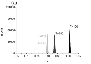
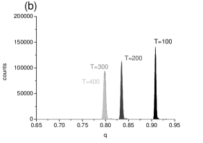
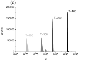
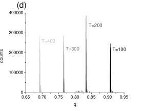
Figure 1: Distribution of similarity coefficients for the DH model with (a) 50,000, (b) 100,000 and (c) 200,000 genes. Panel (d) shows the result for original DH model with infinite genes. The distribution is shown after $T=100$, $200$, $300$ and $400$ generations. In all cases $M=1000$, $\mu=1/4000$ and $q_{min}=0.8$.

The only condition for speciation in the DH model is $q_{mim}>q_{0}\approx(1+4\mu M)^{-1}$ higgs_stochastic_1991 . Changing the mutation rate (or the population size) but keeping $\mu M$ fixed only affects the time to speciation, which increases approximately linearly with $M$, or $1/\mu$, as shown in Fig. 2(a). This is consistent with Eqs.(3) and (4), which indicade that the change in the similarity matrix per time step is proportional to $\mu$ for $\mu\ll 1$. Increasing $\mu M$, on the other hand, decreases $q_{0}$ and increases the number of species formed higgs_stochastic_1991 ; higgs_genetic_1992 .

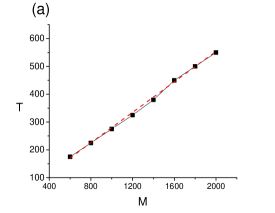
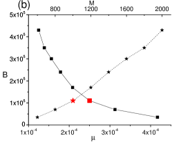
Figure 2: (color online) (a) Time to speciation as a function of population size in the DH model. Dashed line (red) shows a linear fit. (b) Minimum genome size for speciation in the finite genome model as a function of $M$ (stars, upper horizontal axis) and $\mu$ (squares, lower horizontal axis). The values $M=1000$ and $\mu=0.00025$ used in the other figures are marked with a larger (red) symbol. In both panels $4\mu M=1$.

III The DH model with finite genomes

An important feature of the DH model is that there is no need to describe the genomes explicitly: all it takes is the initial similarity matrix $q$, which is set to 1, and the update rule Eq. (4). To implement the model with a finite number of genes it is necessary to keep track of all the $M$ genomes at each generation and calculate the similarities from the definition Eq. (1). Offspring for the next generation are created by choosing (gene by gene) the allele of each parent with equal probability and letting the allele mutate (from +1 to -1 or vice-versa) with probability $\mu$. Parents are chosen like in the original DH model, picking the first parent at random and a second parent compatible with it.

If the number $B$ of genes is small the distribution of similarities starts from $q=1$ and moves to the left until $q=q_{min}$, where it remains stationary and no speciation occurs. We found that speciation only occurs for very large values of $B$, as shown in Fig. 1 (a)-(c). For the parameters used ($M=1000$, $\mu=0.00025$) we observed speciation only for $B$ larger than about $110000$. When compared to the DH model we see that the finite number of genes blurs the peaks of the $q$ distribution, preventing them from breaking up.

The minimum number of genes required for speciation depends directly on the mutation rate and population size. Figure 2(b) shows the minimum value of $B$ for speciation as a function of $M$ and $\mu$ for $4\mu M=1$. For populations with only $M=600$ individuals $B$ drops to about 35000 whereas for $M=2000$ it is necessary at least 430000 genes, showing that $B$ rapidly grows with population sizes. In all cases the simulations were ran for at least twice the time to speciation of the DH model, Fig. 2(a) to make sure the similarity distribution would either move to the left of $q_{min}$ and speciate (for large enough $B$) or stay frozen close to $q=q_{min}$. Error bars for $B$ are of the order of symbols size: $\pm 10^{4}$ for $B\geq 10^{5}$ and $\pm 5\times 10^{3}$ for $B<10^{5}$.

IV Spatial model with finite genomes

The importance of space in evolution has long been recognized Wright-1943 ; Rosen-1995 ; coyne_speciation_2004 ; nostil_2012 and explicit empirical evidence of its role has been recently provided by ring species irwin_speciation_2005 ; martins_evolution_2013 ; Martins-2016 . The spatial model we discuss here is a simplified version of the model proposed in de_aguiar_global_2009 . The main additional ingredient with respect to the DH model with finite genomes is that the individuals are now distributed on a two-dimensional $L\times L$ square area with periodic boundary conditions. Mating is not only restricted by genetic similarity but also by spatial proximity, so that an individual can only choose as mating partner those inside a circular neighborhood of radius $S$ centered on its spatial location, called the mating neighborhood. We note that a number of other effects, such as demographic stochasticity mckane2016 , population expansions martins_evolution_2013 ; Goodsman-2014 , costs of reproduction lecunff-2014 , and migration rates between subpopulations Yamaguchi-2013 might also influence the outcome of speciation. Here we consider only the effect of finite mating neighborhoods and keep all the other ingredients as similar as possible to the original DH model.

Figure 3: Minimum number of genes required for speciation as a function of the mating neighborhood radius $S$. The top axis show the corresponding average number of individuals in the mating neighborhood ($M=1000$, $\mu=1/4000$.)

Space represents an environment where resources are distributed homogeneously and the individuals should occupy it more or less uniformily so that enough resources would be available to all of them. The total carrying capacity is the population size $M$ and the average area needed per individual is $M/L^{2}$. The dynamics is constructed in such a way that offspring are placed close to the location of the original parents and the approximately uniform distribution of the population is preserved at all times. However, the mechanism used in the DH model of picking a random individual from the population to be the first parent and then a second individual to be the second parent (and repeating the process $M$ times) promotes strong spatial clustering.

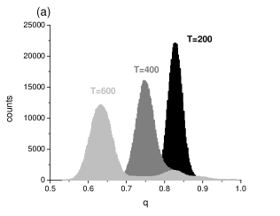
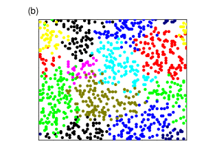
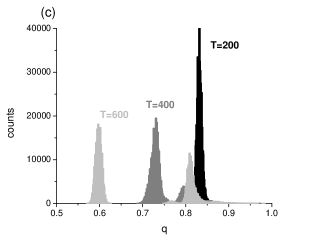
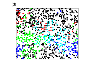
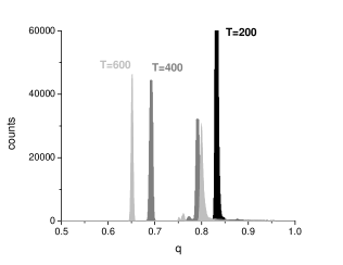
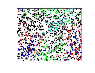
Figure 4: (color online) (a) Distribution of similarity coefficients for the spatial model with $B=1000$, $q_{min}=0.8$ and $S=7$ for $T=200$, $400$ and $600$ generations. (b) Spatial distribution of the population at $T=600$; different colors (shades of gray) show different species. Panels (c) and (d) show similar plots for $B=10000$ and $S=11$; (e) and (f) show the results for $B=100000$ and $S=14$.

In order to avoid clustering we implement the dynamics in a slightly different way de_aguiar_global_2009 (see also section V): the initial population is randomly placed in the $L\times L$ area. Each one of the $M$ individuals has a chance of reproducing but there is a probability $Q$ that it will not do so, accounting for the fact that not all individuals in the present generation will be first parents of the next. In the case the focal individual does not reproduce, another one from its mating neighborhood is randomly chosen to reproduce in its place. In either case the offspring generated will be positioned exactly at the location of the focal individual or will disperse with probability $D=0.01$ to one of 20 neighboring sites. Therefore, close to the location of every individual of the previous generation there will be an individual in the present generation, keeping the spatial distribution uniform and avoiding the formation of clusters. The first parent (or a neighbor reproducing in its place) chooses a compatible second parent within its mating neighborhood of radius $S$. If $S$ is small, the number of individuals in the mating neighborhood can be close to zero due to fluctuations in the spatial distribution. To avoid this situation, and also to follow the procedure introduced in de_aguiar_global_2009 , if the number of compatible mates in the neighborhood is smaller than $P$ ($P=3$ in the simulations), the individual expands the search radius to $S+1$. If the number of compatible mates is still smaller than $P$, the process is repeated twice more up to $S+3$, and if there is still less than $P$ potential mates another neighbor is randomly selected to reproduce in its place de_aguiar_global_2009 . The probability $Q$ was fixed in $Q=e^{-1}\approx 0.37$, which corresponds approximately to the probability that an individual is not selected in $M$ trials with replacement, $(1-1/M)^{M}\approx e^{-1}$, in accordance with the DH model.

The size of mating neighborhood is a key extra parameter. If $S\simeq L$ we recover the DH model with finite genomes. If $S$ is small speciation is strongly facilitated and can occur for much smaller values of $B$ for a given $q_{min}$ or $G/B$. Fig. 3 shows the minimum value of $B$ for which speciation happens as a function of the size of the mating neighborhood $S$ for $q_{min}=0.8$. The figure also shows the average number of individuals inside the mating neighborhood, $M_{S}=M\pi S^{2}/L^{2}$. The values were obtained by varying $S$ by units of $0.5$ when $B\leq 1000$ and by units of $2$ for larger $B$’s. Populations evolved for $T=600$ generations. In some cases speciation did occur for slightly smaller values of $B$, but it took much longer times. For $B=1000$, for instance, we observed speciation for $S=8$ for $T\approx 3000$. Comparing with the finite DH model we note that speciation can take place even for $B=100$ if $S\leq 5$. As $B$ increases the restriction in the size of the mating neighborhood required for speciation decreases, until it is unnecessary if $B$ is of the order of 110000.

Figure 4 shows the histogram of similarity between pairs of individuals at three times and a snapshot of the population for $B=1000$, $S=7$; $B=10000$, $S=11$ and $B=100000$ and $S=14$. The peaks in the distribution are larger both because $B$ is small and because of the restriction in $S$. For $B=1000$ the species are well localized in space, with little overlap at their boundaries (see de_aguiar_global_2009 ). For $B=10000$ and $B=100000$ the spatial overlap between species is considerably larger.

V Spatial model with very large genomes

As discussed in section IV, the construction of spatial models that converge to the finite DH model as the parameter S becomes large is not straightforward. The problem resides in the way generations are constructed in the DH model, where a first parent is chosen at random from the population and then a second, genetically compatible, parent is also chosen at random to generate an offspring. The direct application of this procedure in the spatial model would consist in choosing a random first parent and picking the second parent from its mating neighborhood, an area $\pi S^{2}$ centered on the individual. The offspring should be put close to the location of the first or second parent, or somewhere in between. This, however, leads to spatial clustering of the population, since a large fraction ($\approx e^{-1}$) of the population is never chosen as first parents, leaving holes in these areas and overcrowding areas where individuals are picked twice or more. To avoid this situation we have replaced the random choice of the first parent by going through the population one by one and giving each individual a chance ($1-e^{-1}$) to reproduce. When it did not we picked another individual from its mating neighborhood to reproduce in its place, instead of a random individual taken from the entire population as in the original DH or finite DH models. The offspring is always placed close to the location of the first parent, keeping the distribution spatially uniform.

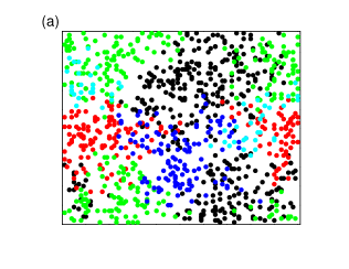
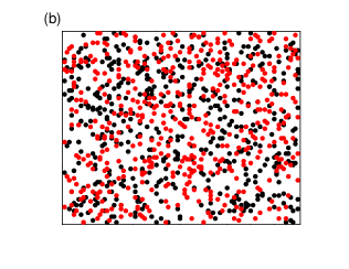
Figure 5: (color online) Spatial distribution of the population for $B=200000$ at $T=300$ for (a) $S=10$ and (b) $S=40$. Small mating neighborhoods favors spatial isolation of species.

In order to compare the spatial model with an equivalent sympatric system we implemented a variation of the finite DH model in which, similarly to the spatial model, we give each individual a chance ($1-e^{-1}$) to reproduce and, when it does not, we pick another random individual from the entire population to reproduce in its place. The results obtained with this variation are qualitatively identical to those described in sections II and III. This validates the comparison of the DH finite genome model with the spatial model introduced in section IV.

Finally we consider the process of speciation in the spatial model for genome sizes $B$ above the threshold where speciation occurs in the sympatric model. In this case speciation occurs for any value of $S$, small or large. For small $S$ local mating creates a spatial distribution of genotypes where nearby individuals tend to be similar but different from others located far away de_aguiar_global_2009 . For finite populations this genetic gradient is not smooth, but step-like, and prone to break up into genetically isolated groups that are spatially correlated. Speciation happens not because $B$ is large, but because $S$ is small. For large $S$, on the other hand, the mechanism is very different and takes place on the global scale of the population. The balance between mutations, which generally increases the average genetic distance between two individuals, and sexual reproduction, which mixes the genomes and has the opposite effect, leads to a distribution of genetic distances in the population. Only when this distribution becomes wide enough, as compared with the criterion of assortative mating, the population splits into species. Figure 5 shows the resulting populations in each case, where a signature of $S$ is clearly seen in the spatial organization of the species.

VI Discussion

The mechanisms responsible for the origin of species remain controversial Chung_2004 . Among the important questions yet to be fully understood is the role of geography (allopatric, parapatric and sympatric modes) and the number of genes involved in the evolution of reproductive isolation. It has been recently argued that these two points are closely related and that detailed molecular analysis might reveal the geographic mode behind specific speciation events Machado_2002 .

Sympatric speciation has been thought to be the most unlikely of the modes, since the possibility of constant gene flow would keep the populations mixed and prevent the evolution of reproductive barriers Bolnick_2007 . Dieckmann and collaborators have argued that this is not so if competition for resources is strong enough Dieckmann_1999 ; Dieckmann_2003 ; Doebeli_2005 . In that case reproductive isolation would not only evolve naturally but would require sympatry, otherwise competition for local resources would not be intense Dieckmann_1999 .

Surprisingly, Derrida and Higgs have shown that sympatric speciation may occur even without competition, in a totally neutral scenario, if mating is assortative and if the number of loci in the genome can be considered infinite higgs_stochastic_1991 . When loci are interpreted as genes the hypothesis of an infinitely large genome becomes rather unrealistic. However, at the molecular level, where nucleotide sequences are the units to be considered, infinite loci models become attractive Kimura_1964 ; Ewens_1979 . Nevertheless, nucleotides can hardly be considered independent and certainly do not segregate in the way as assumed by the DH models. Understanding how many independently segregating loci are necessary for neutral sympatric speciation is, therefore, an important question. The main parameters controlling the dynamics in the DH model are $q_{0}=(1+4\mu M)^{-1}$ and the assortativity measure $q_{min}$. The combination $\theta=2\mu M$ also appears in Hubbell’s neutral theory of biodiversity Hubbell-2001 and is the fundamental biodiversity number, since it controls the number of species in a community and the abundance distribution.

In this paper we have revisited the DH model and simulated it for finite numbers of loci. We found that, for typical parameters used in the original paper, speciation happens only for very large number of loci, of the order of $10^{5}$. When the number of loci is small, the genetic variability within the population is large, hindering speciation. The histogram of genetic similarity between individuals evolves into a broad peak instead of multiple sharp peaks that represent groups of very similar individuals that are dissimilar among different groups. As the number of genes increase the peaks become thiner, secondary structures appear and eventually turn into species. Increasing the mutation rate and keeping $\mu M$ fixed decreases the minimum number of loci needed and also the time to speciation.

In contrast with the sympatric DH model, the spatial model introduced in de_aguiar_global_2009 displays speciation with much smaller number of loci. The model considers a population that is uniformly distributed in space, without any explicit separation into demes or subpopulations. Although it falls into the class of parapatric models, it has been termed topopatric to distinguish it from models involving demes or metapopulations Manzo_Peliti_1994 . Mating is restricted not only by genetic similarity but also by spatial proximity, allowing gene flow across the entire population but substantially reducing the speed of the flow. Mutations are transmitted diffusively across the population, and not instantaneously like in the sympatric model, largely facilitating speciation Schneider2016 . Previous studies with metapopulation models (and infinitely large genomes) observed similar effects, with speciation occurring for smaller mutation rates due to the isolation of subpopulations Manzo_Peliti_1994 . For small number of genes, of the order of 100, speciation occurs only with severe spatial mating restrictions. Accordingly, the species that form display strong spatial segregation, with little overlap between adjacent species (Figs. 4(b) and 5(a)). This type of geographic distribution leads back to question of modes of speciation and suggests that it might happen that species appeared not because the populations were geographically separated (as in allopatry) but rather they are geographically separated because they emerged in a homogeneous environment with slow gene flow. If the number of loci participating in the assortative process is large the spatial restriction on mating can be relaxed. As a consequence, the spatial segregation decreases and the overlap among species increases.

Acknowledgments:

It is a pleasure to thank David M. Schneider, Ayana Martins and Blake Stacey for their critical reading of this paper and many suggestions. This work was partly supported by the Brazilian agencies FAPESP (grant 2016/06054-3) and CNPq (grant 302049/2015-0).

References

- (1) E. Mayr. Systematics and the origin of species. Columbia University Press, New York, 1942.
- (2) Jerry A. Coyne and H. Allen Orr. Speciation. Sinauer Associates, Inc., 1 edition, May 2004.
- (3) Patrick Nosil. Ecological Speciation. Oxford University Press, 1 edition, 2012.
- (4) Mark Kirkpatrick and Scott L Nuismer. Sexual selection can constrain sympatric speciation. Proceedings of the Royal Society B: Biological Sciences, 271(1540):687–693, 04 2004.
- (5) Daniel I. Bolnick and Benjamin M. Fitzpatrick. Sympatric speciation: Models and empirical evidence. Annual Review of Ecology, Evolution, and Systematics, 38(1):459–487, 2007.
- (6) Alexey S. Kondrashov and Mikhail V. Mina. Sympatric speciation: when is it possible? Biological Journal of the Linnean Society, 27(3):201–223, 1986.
- (7) Daniel Udovic. Frequency-dependent selection, disruptive selection, and the evolution of reproductive isolation. The American Naturalist, 116(5):621–641, 1980.
- (8) Joseph Felsenstein. Skepticism towards santa rosalia, or why are there so few kinds of animals? Evolution, 35(1):124–138, 1981.
- (9) A S Kondrashov and M Shpak. On the origin of species by means of assortative mating. Proceedings of the Royal Society B: Biological Sciences, 265(1412):2273–2278, 12 1998.
- (10) Alexey S. Kondrashov and Fyodor A. Kondrashov. Interactions among quantitative traits in the course of sympatric speciation. Nature, 400(6742):351–354, 07 1999.
- (11) M. Doebeli. Adaptive speciation when assortative mating is based on female preference for male marker traits. Journal of Evolutionary Biology, 18(6):1587–1600, 2005.
- (12) Sergey Gavrilets. The maynard smith model of sympatric speciation. Journal of Theoretical Biology, 239(2):172 – 182, 2006. Special Issue in Memory of John Maynard SmithSpecial Issue in Memory of John Maynard Smith.
- (13) Ulf Dieckmann and Michael Doebeli. On the origin of species by sympatric speciation. Nature, 400(6742):354–357, 07 1999.
- (14) Sergey Gavrilets. Fitness Landscapes and the Origin of Species (MPB-41). Princeton University Press, July 2004.
- (15) N. H. Barton and J. Polechova. The limitations of adaptive dynamics as a model of evolution. Journal of Evolutionary Biology, 18(5):1186–1190, 2005.
- (16) Daniel I. Bolnick. Waiting for sympatric speciation. Evolution, 58(4):895–899, 2004.
- (17) Sergey Gavrilets. “adaptive speciation”—it is not that easy: Reply to doebeli et al. Evolution, 59(3):696–699, 2005.
- (18) P. G. Higgs and B. Derrida. Stochastic models for species formation in evolving populations. Journal of Physics A: Mathematical and General, 24(17):L985, September 1991.
- (19) Paul G. Higgs and Bernard Derrida. Genetic distance and species formation in evolving populations. Journal of Molecular Evolution, 35(5):454–465, November 1992.
- (20) M Kimura and J. F. Crow. The number of alleles that can be maintained in a finite population. Genetics, 49:725–738, 1964.
- (21) W. J. Ewens. Mathematical population genetics. Springer-Verlag Berlin ; New York, 1979.
- (22) M. A. M. de Aguiar, M. Baranger, E. M. Baptestini, L. Kaufman, and Y. Bar-Yam. Global patterns of speciation and diversity. Nature, 460(7253):384–387, July 2009.
- (23) Marcus A. M. de Aguiar, David M. Schneider, Eduardo do Carmo, Paulo R. A. Campos, and Ayana B. Martins. Error catastrophe in populations under similarity-essential recombination. Journal of Theoretical Biology, 374:48–53, June 2015.
- (24) Sewall Wright. Isolation by distance. Genetics, 28(2):114–138, 1943.
- (25) Michael L. Rosenzweig. Species diversity in space and time. Cambridge University Press Cambridge ; New York, 1995.
- (26) Darren E. Irwin, Staffan Bensch, Jessica H. Irwin, and Trevor D. Price. Speciation by distance in a ring species. Science, 307(5708):414–416, January 2005.
- (27) Ayana B. Martins, Marcus A. M. de Aguiar, and Yaneer Bar-Yam. Evolution and stability of ring species. Proceedings of the National Academy of Sciences, 110(13):5080–5084, March 2013.
- (28) Ayana B. Martins and Marcus A. M. de Aguiar. Barriers to gene flow and ring species formation. Evolution, doi:10.1111/evo.13121, 2016.
- (29) L. F. Lafuerza and A. J. McKane. Role of demographic stochasticity in a speciation model with sexual reproduction. Phys. Rev. E, 93(3):032121, March 2016.
- (30) Devin W. Goodsman, Barry Cooke, David W. Coltman, and Mark A. Lewis. The genetic signature of rapid range expansions: How dispersal, growth and invasion speed impact heterozygosity and allele surfing. Theoretical Population Biology, 98:1 – 10, 2014.
- (31) Yann Le Cunff and Khashayar Pakdaman. Reproduction cost reduces demographic stochasticity and enhances inter-individual compatibility. Journal of Theoretical Biology, 360:263 – 270, 2014.
- (32) Ryo Yamaguchi and Yoh Iwasa. First passage time to allopatric speciation. Interface Focus, 3(6), 2013.
- (33) Chung-I Wu and Chau-Ti Ting. Genes and speciation. Nat Rev Genet, 5(2):114–122, 02 2004.
- (34) Carlos A Machado, Richard M Kliman, Jeffrey A Markert, and Jody Hey. Inferring the history of speciation from multilocus dna sequence data: the case of drosophila pseudoobscura and close relatives. Mol Biol Evol, 19(4):472–88, Apr 2002.
- (35) Michael Doebeli and Ulf Dieckmann. Speciation along environmental gradients. Nature, 421(6920):259–264, 01 2003.
- (36) Stephen P. Hubbell. The Unified Neutral Theory of Biodiversity and Biogeography (MPB-32). Princeton University Press, 2001.
- (37) F Manzo and L Peliti. Geographic speciation in the derrida-higgs model of species formation. Journal of Physics A: Mathematical and General, 27(21):7079, 1994.
- (38) David M. Schneider, Ayana B. Martins, and Marcus A.M. de Aguiar. The mutation-drift balance in spatially structured populations. Journal of Theoretical Biology, 402:9 – 17, 2016.