Strain tensor selection and the elastic theory of incompatible thin sheets

Abstract

The existing theory of incompatible elastic sheets uses the deviation of the surface metric from a reference metric to define the strain tensor [Efrati et al., J. Mech. Phys. Solids 57, 762 (2009)]. For a class of simple axisymmetric problems we examine an alternative formulation, defining the strain based on deviations of distances (rather than distances squared) from their rest values. While the two formulations converge in the limit of small slopes and in the limit of an incompressible sheet, for other cases they are found not to be equivalent. The alternative formulation offers several features which are absent in the existing theory. (a) In the case of planar deformations of flat incompatible sheets, it yields linear, exactly solvable, equations of equilibrium. (b) When reduced to uniaxial (one-dimensional) deformations, it coincides with the theory of extensible elastica; in particular, for a uniaxially bent sheet it yields an unstrained cylindrical configuration. (c) It gives a simple criterion determining whether an isometric immersion of an incompatible sheet is at mechanical equilibrium with respect to normal forces. For a reference metric of constant positive Gaussian curvature, a spherical cap is found to satisfy this criterion except in an arbitrarily narrow boundary layer.

I Introduction

In the past two decades there has been a renewed interest in the elasticity of thin solid sheets in view of the wealth of surface patterns and three-dimensional (3D) shapes that they exhibit under stress Cerda and Mahadevan (2003); Huang et al. (2010); Davidovitch et al. (2011); Vandeparre et al. (2011); Cerda and Mahadevan (1998); Brau et al. (2013); King et al. (2012); Audoly (2011); Cerda and Mahadevan (2005). In addition, experiments and models have been devised for incompatible sheets, which contain internal residual stresses even in the absence of external forces Marder et al. (2003); Sharon et al. (2002); Efrati et al. (2009a, b); Sharon and Efrati (2010); Efrati et al. (2007); Klein et al. (2007); Efrati et al. (2013); Dervaux et al. (2009); Marder (2003); Pezzulla et al. (2015); Dervaux and Ben-Amar (2008); Santangelo (2009); Dias et al. (2011); Audoly and Boudaoud (2003); Guven et al. (2012); Müller et al. (2008); Ben-Amar and Goriely (2005); Goriely and Ben Amar (2005); Lewicka et al. (2010). The study of such sheets has been motivated by their relevance to morphologies in nature Marder et al. (2003); Marder (2003); Dervaux et al. (2009); Dervaux and Ben-Amar (2008); Armon et al. (2014) and frustrated self-assembly Armon et al. (2014); Grossman et al. (2016). Incompatible sheets form nontrivial 3D shapes spontaneously. They can also be “programmed” to develop a desired 3D shape Klein et al. (2007, 2011); Dias et al. (2011); Oppenheimer and Witten (2015); Kim et al. (2012); Bae et al. (2014).

The necessary existence of sheets with unremovable internal stresses is rationalized as follows. When treating a thin solid sheet as a mathematical surface, its relaxed state is characterized by a 2D reference metric tensor, $\bar{g}_{\alpha\beta}$, associated with the relaxed in-plane configuration, and a reference second fundamental form, $\bar{b}_{\alpha\beta}$, related to the relaxed out-of-plane configuration (curvature) Efrati et al. (2009a). (We shall use Latin indices $(i,j,\ldots)$ for 3D coordinates and Greek indices $(\alpha,\beta,\ldots)$ for 2D ones.) However, not any $\bar{g}_{\alpha\beta}$ and $\bar{b}_{\alpha\beta}$ correspond to a physical surface. For the surface to be embeddable in 3D Euclidean space, these forms must satisfy a set of geometrical constraints (Lipschutz, 1969, p. 203). Thus, in general, an actual sheet will be incompatible — its actual metric and second fundamental form, $a_{\alpha\beta}$ and $b_{\alpha\beta}$, will not coincide with their reference counterparts — leading to unavoidable intrinsic stresses.

A covariant theory for incompatible elastic bodies has been presented by Efrati, Sharon, and Kupferman (referred to hereafter as ESK) Efrati et al. (2009a) and successfully applied to several experimental systems Armon et al. (2014); Moshe et al. (2015a); Grossman et al. (2016). Their elastic energy for a 3D body reads,

$$E_{\rm 3D}=\int_{\mathcal{V}}\mathcal{A}^{ijkl}\tilde{\epsilon}_{ij}\tilde{\epsilon}_{kl}\sqrt{|\bar{g}|}dV,$$

$$\tilde{\epsilon}_{ij}=\frac{1}{2}(g_{ij}-\bar{g}_{ij}),$$ (1)

where the integration is over the unstrained volume, $\mathcal{V}$, $g_{ij}$ and $\bar{g}_{ij}$ are the metric and reference metric, $\bar{g}$ is the determinant of the reference metric and $\mathcal{A}^{ijkl}$ is the elastic tensor. To explicitly distinguish the strain used by ESK we mark it with a tilde. ESK also presented a dimensional reduction of this energy to 2D for incompatible thin elastic sheets, resulting in a sum of stretching and bending contributions,

$$\text{ESK:}\ \ \ E_{\rm 2D} = E_{s}+E_{b}=\frac{t}{2}\int_{A}\mathcal{A}^{\alpha\beta\gamma\delta}\tilde{\epsilon}_{\alpha\beta}\tilde{\epsilon}_{\gamma\delta}\sqrt{|\bar{g}|}dA+\frac{t^{3}}{24}\int_{A}\mathcal{A}^{\alpha\beta\gamma\delta}b_{\alpha\beta}b_{\gamma\delta}\sqrt{|\bar{g}|}dA,$$

$$\ \ \ \tilde{\epsilon}_{\alpha\beta} = \frac{1}{2}(a_{\alpha\beta}-\bar{g}_{\alpha\beta}),$$ (2)

where $t$ is the sheet thickness, the integral is over the unstrained area, and $\tilde{\epsilon}_{\alpha\beta}$ is the ESK two-dimensional strain tensor.

Arguably, the functional in Eq. (1) represents the simplest covariant theory of incompatible elasticity. It makes a certain choice of strain tensor, which is based on the relative deviations of the distances squared from their rest values (the so-called Green–St. Venant strain tensor Efrati et al. (2009a); Fu and Ogden (2001); Dill (2007)). In elasticity theory the strain measure is regarded as a parametrization freedom — so long as the stress tensor (and resulting energy functional) is appropriately defined, different definitions of the strain tensor will lead to the same equilibrium deformation of the elastic body (Dill, 2007, Sec. 2.5). Indeed, other choices of strain have been made in compatible elasticity, such as the Biot strain tensor Biot (1965), which expresses the spring-like deviations of distances within the body. Generally, one can write a dimensionless deviation of a certain variable $\ell$ from its reference $\ell_{0}$ as $\Delta=\frac{1}{m\ell_{0}^{m}}\left(\ell^{m}-\ell_{0}^{m}\right)$, where $m$ is an arbitrary number (Fu and Ogden, 2001, p. 6). In the limit of small deviations, $\Delta\ll 1$, one always gets $\Delta\simeq(\ell-\ell_{0})/\ell_{0}$ for any $m$. Thus, it seems that within linear elasticity of infinitesimal strains the choice of $m$ is immaterial.

Dimensional reduction of 3D linear elasticity to 2D thin sheets introduces non-quadratic terms in the reduced energy functional. As we shall see below, a different selection of the strain tensor for the 3D body — the incompatible analogue of Biot’s strain — leads to non-quadratic terms in 2D which differ from those obtained from Eq. (2). Thus, the resulting theory is not equivalent to the ESK one. This holds even in the case of a compatible sheet with a flat reference metric Koiter and Simmonds (1973); Ciarlet (2005). The differences between the two formulations are quantitatively small but have a qualitative effect on the structure of the theory and the simplicity of its application. We note that the present work is not the first to indicate the effect of strain-tensor selection. Similar observations were made in the context of compatible beam theory Irschik and Gerstmayr (2009).

We begin in Sec. II by presenting the alternative formulation based on Biot’s selection of 3D strain. We perform a reduction to 2D, which is limited to axisymmetric surface deformations along the principal axes of stress. In Sec. III we apply the formulation to the simple example of a compatible sheet that is uniaxially bent by boundary moments. We show that it coincides in this case with the extensible elastica, yielding a bent, unstrained, cylindrical shape, whereas the choice made in Eq. (I) gives a cylinder with non-zero in-plane strain. Section IV presents further applications to several examples of incompatible flat discs. We derive linear equations of equilibrium, and obtain their analytical solutions, for problems which are described by nonlinear equations in the ESK theory. Section V presents a self-consistency criterion, based on the alternative formulation, for the stability of axisymmetric isometric immersions of such discs with respect to internal bending moments. We apply the criterion to the case of a reference metric with constant positive Gaussian curvature, whose isometric immersion is a spherical cap. In Sec. VI we conclude and discuss future extensions of this work.

II Alternative two-dimensional formulation for simple deformations

We impose three requirements on the alternative formulation for 2D incompatible sheets: (a) It should be invariant under rigid transformations (rotations and translations). (b) In the limit of incompressibe compatible sheets it should converge to the known Willmore functional Efrati et al. (2009a). (c) In the small-slope approximation it should converge to the Föppl-von Kàrmàn (FvK) theory Landau and Lifshitz (1986).

The formulation presented here holds for a small subset of problems which we can treat exactly. We consider a disc-like thin sheet of radius $R$, and parametrize it by the polar coordinates $(r,\theta)$. The relaxed length, squared, of a line element on the sheet is given by the following reference metric,

$$\bar{g}_{\alpha\beta}=\begin{pmatrix}1&0\\ 0&\Phi^{2}(r)\end{pmatrix}\ \ \ ,\ \ \ ds^{2}=dr^{2}+\Phi^{2}(r)d\theta^{2},$$ (3)

where $dr$ is the relaxed arclength element along the radial direction and $2\pi\Phi(r)$ is the relaxed perimeter of a circle of radius $r$ around the disc center. Once $\Phi(r)\neq r$ the flat configuration contains internal strains. While such a sheet may have a complicated equilibrium deformation, we restrict ourselves to surfaces of revolution. The 3D position of a displaced point on the surface is given by

$${\bf f}(r,\theta)=[r+u_{r}(r)]{\bf\hat{r}}+\zeta(r){\bf\hat{z}},$$ (4)

where $u_{r}$ is the radial displacement, $\zeta$ is the height function, $\hat{{\bf r}}$ is a unit vector tangent to the sheet in the radial direction, and $\hat{{\bf z}}$ is a unit vector in the perpendicular direction to the flat disc. Note that, for an incompatible sheet, the case of $u_{r}(r)=\zeta(r)=0$ does not correspond to a stress-free configuration.

The 2D energy functional of this system can be derived out of a 3D formulation using the Kirchhoff-Love hypothesis Love (1927); Gol’Denveizer (1961); Libai and Simmonds (1988); Efrati et al. (2009a); Koiter and Simmonds (1973); Dias et al. (2011). For this purpose we identify the 2D sheet defined above with the mid-surface of a 3D slab. Under the Kirchhoff-Love set of assumptions the configuration of the 3D body is given by,

$${\bf f}^{\star}(r,\theta,x_{3})={\bf f}(r,\theta)+x_{3}\hat{{\bf n}}(r,\theta),$$ (5)

where $x_{3}\in[-t/2,t/2]$ is a coordinate in the direction ${\bf\hat{n}}$ normal to the mid-surface,

$${\bf\hat{n}}=\frac{\partial_{r}{\bf f}\times\partial_{\theta}{\bf f}}{|\partial_{r}{\bf f}\times\partial_{\theta}{\bf f}|}=\frac{(1+\partial_{r}u_{r}){\bf\hat{z}}-\partial_{r}\zeta{\bf\hat{r}}}{\sqrt{(1+\partial_{r}u_{r})^{2}+(\partial_{r}\zeta)^{2}}}.$$ (6)

On a surface of constant $x_{3}$, the length squared of an infinitesimal line element is found, after some algebra, to be,

$$d{\bf f^{\star}}^{2}=\left[a_{rr}-2x_{3}b_{rr}+x_{3}^{2}c_{rr}\right]dr^{2}+\left[a_{\theta\theta}-2x_{3}b_{\theta\theta}+x_{3}^{2}c_{\theta\theta}\right]d\theta^{2},$$ (7)

where $a_{\alpha\beta}=\partial_{\alpha}{\bf f}\cdot\partial_{\beta}{\bf f}$, $b_{\alpha\beta}=-\partial_{\alpha}{\bf f}\cdot\partial_{\beta}\hat{{\bf n}}$, and $c_{\alpha\beta}=\partial_{\alpha}\hat{{\bf n}}\cdot\partial_{\beta}\hat{{\bf n}}$, are the first, second, and third fundamental forms.

On the other hand, following Biot’s approach (Biot, 1965, p. 17), a pure deformation of that surface is represented by the symmetric transformation matrix,

$$\begin{pmatrix}dr^{\prime}\\ \Phi d\theta^{\prime}\end{pmatrix}=\begin{pmatrix}1+\epsilon^{\star}_{rr}&\epsilon^{\star}_{r\theta}\\ \epsilon^{\star}_{r\theta}&1+\epsilon^{\star}_{\theta\theta}\end{pmatrix}\begin{pmatrix}dr\\ \Phi d\theta\end{pmatrix},$$ (8)

where $\epsilon_{\alpha\beta}^{\star}$ is the in-plane strain tensor of the constant-$x_{3}$ surface. Note that this definition of the strain correponds to changes in length (not length squared). Thus,

$$d{\bf f^{\star}}^{2} = dr^{\prime 2}+(\Phi d\theta^{\prime})^{2}$$ (9)

$$= \left[(1+\epsilon^{\star}_{rr})^{2}+(\epsilon^{\star}_{r\theta})^{2}\right]dr^{2}+\left[(1+\epsilon^{\star}_{\theta\theta})^{2}+(\epsilon^{\star}_{r\theta})^{2}\right](\Phi d\theta)^{2}+2\epsilon^{\star}_{r\theta}(2+\epsilon^{\star}_{rr}+\epsilon^{\star}_{\theta\theta})\Phi d\theta dr.$$

Comparinging Eqs. (7) and (9), we identify,

$$\epsilon_{rr}^{\star}=\sqrt{(1+\epsilon_{rr})^{2}-2x_{3}b_{rr}+x_{3}^{2}c_{rr}}-1,$$ (10a)

$$\epsilon_{\theta\theta}^{\star}=\sqrt{(1+\epsilon_{\theta\theta})^{2}-2x_{3}b_{\theta\theta}/\Phi^{2}+x_{3}^{2}c_{\theta\theta}/\Phi^{2}}-1,$$ (10b)

$$\epsilon_{r\theta}^{\star}=0,$$ (10c)

where

$$\epsilon_{rr}=\sqrt{a_{rr}}-1=\sqrt{(1+\partial_{r}u_{r})^{2}+(\partial_{r}\zeta)^{2}}-1,$$ (11a)

$$\epsilon_{\theta\theta}=\sqrt{a_{\theta\theta}}/\Phi-1=\frac{r}{\Phi}-1+\frac{u_{r}}{\Phi}.$$ (11b)

We have reached a definition of the mid-surface in-plane strains in terms of the actual and reference metrics, based on the spring-like deformed length rather than length squared.

The geometrical interpretation of these strains is illustrated in Fig. 1. The fact that the strains describe deformed lengths (Gol’Denveizer, 1961, p. 41) leads at this stage to two simplifications. First, the fundamental forms satisfy the simple relations, $c_{rr}=b_{rr}^{2}/(1+\epsilon_{rr})^{2}$ and $\Phi^{2}c_{\theta\theta}=b_{\theta\theta}^{2}/(1+\epsilon_{\theta\theta})^{2}$. Second, once these expressions are substituted in Eqs. (10), we can rewrite the strains at constant $x_{3}$ as,

$$\epsilon_{rr}^{\star}=\epsilon_{rr}-x_{3}\phi_{rr},$$ (12a)

$$\epsilon_{\theta\theta}^{\star}=\epsilon_{\theta\theta}-x_{3}\phi_{\theta\theta}.$$ (12b)

(See Fig. 1c for the geometrical meaning of these strains.) Here we have defined the out-of-plane strains,

$$\phi_{rr}=\sqrt{c_{rr}}=\frac{(1+\partial_{r}u_{r})\partial_{rr}\zeta-\partial_{rr}u_{r}\partial_{r}\zeta}{(1+\partial_{r}u_{r})^{2}+(\partial_{r}\zeta)^{2}},$$ (13a)

$$\phi_{\theta\theta}=\sqrt{c_{\theta\theta}}/\Phi=\frac{1}{\Phi}\frac{\partial_{r}\zeta}{\sqrt{(1+\partial_{r}u_{r})^{2}+(\partial_{r}\zeta)^{2}}}.$$ (13b)

Defining further $\phi^{r}$ and $\phi^{\theta}$ as the tangent angles in the radial and azimuthal directions of the surface of revolution, we find $\phi_{rr}=\partial_{r}\phi^{r}$ and $\phi_{\theta\theta}=(1/\Phi)\partial_{\theta}\phi^{\theta}$ (see Fig. 1(a) and the explanation in its caption). This clarifies the geometrical meaning of the “bending-strains”, $\phi_{rr}$ and $\phi_{\theta\theta}$.

In the framework of linear elasticity the energy functional of the 3D slab is given by Landau and Lifshitz (1986),

$$E_{\rm 3D}=\frac{E}{2(1-\nu^{2})}\int_{-t/2}^{t/2}\int_{0}^{R}\int_{0}^{2\pi}\left[(\epsilon_{rr}^{\star})^{2}+(\epsilon_{\theta\theta}^{\star})^{2}+2\nu\epsilon_{rr}^{\star}\epsilon_{\theta\theta}^{\star}\right]\Phi d\theta drdx_{3},$$ (14)

where $E$ is Young’s modulus and $\nu$ the Poisson ratio. Substituting Eqs. (12) in (14) and integrating over $x_{3}$ gives,

$$E_{\rm 2D}=\frac{Y}{2}\int_{0}^{R}\int_{0}^{2\pi}\left[\epsilon_{rr}^{2}+\epsilon_{\theta\theta}^{2}+2\nu\epsilon_{rr}\epsilon_{\theta\theta}\right]\Phi d\theta dr+\frac{B}{2}\int_{0}^{R}\int_{0}^{2\pi}\left[\phi_{rr}^{2}+\phi_{\theta\theta}^{2}+2\nu\phi_{rr}\phi_{\theta\theta}\right]\Phi d\theta dr,$$ (15)

where $Y=Et/(1-\nu^{2})$ is the stretching modulus and $B=Et^{3}/12(1-\nu^{2})$ is the bending modulus. The first integral in Eq. (15) is the stretching energy,

$$E_{s}=\frac{1}{2}\int_{0}^{R}\int_{0}^{2\pi}\left[\sigma_{rr}\epsilon_{rr}+\sigma_{\theta\theta}\epsilon_{\theta\theta}\right]\Phi d\theta dr,$$ (16)

where the stress components $\sigma_{\alpha\beta}=\delta E/\delta\epsilon_{\alpha\beta}$ are given by,

$$\sigma_{rr}=Y(\epsilon_{rr}+\nu\epsilon_{\theta\theta}),$$ (17a)

$$\sigma_{\theta\theta}=Y(\epsilon_{\theta\theta}+\nu\epsilon_{rr}).$$ (17b)

Similarly, the second integral in Eq. (15) gives the bending energy,

$$E_{b}=\frac{1}{2}\int_{0}^{R}\int_{0}^{2\pi}\left[M_{rr}\phi_{rr}+M_{\theta\theta}\phi_{\theta\theta}\right]\Phi d\theta dr,$$ (18)

where the bending moments, $M_{\alpha\beta}=\delta E/\delta\phi_{\alpha\beta}$, in the radial and azimuthal directions are given by,

$$M_{rr}=B(\phi_{rr}+\nu\phi_{\theta\theta}),$$ (19a)

$$M_{\theta\theta}=B(\phi_{\theta\theta}+\nu\phi_{rr}).$$ (19b)

Figure 1: (a) Deformation of an infinitesimal element in the radial direction. The relaxed length of the element is $dr$ (solid line), and the deformed length is $|\partial_{r}{\bf f}|dr$. The radial strain component is $\epsilon_{rr}=\frac{|\partial_{r}{\bf f}|dr-dr}{dr}$, as given by Eq. (11a). The angle $\phi^{r}$ satisfies $\sin\phi^{r}=\partial_{r}{\bf f}\cdot{\bf\hat{z}}/|\partial_{r}{\bf f}|$. Substituting ${\bf f}(r,\theta)$ from Eq. (4) in the latter relation and using Eq. (13b) gives $\phi_{\theta\theta}=\sin\phi^{r}/\Phi$. In addition, by direct differentiation it can be verified that $\phi_{rr}=\partial_{r}\phi^{r}$ as given by Eq. (13a). (b) Deformation of an infinitesimal sheet element in the azimuthal direction. The relaxed length in this direction is $\Phi d\theta$ (solid line) and the deformed length is $|\partial_{\theta}{\bf f}|d\theta$ (dashed line). Thus, the azimuthal strain is $\epsilon_{\theta\theta}=\frac{|\partial_{\theta}{\bf f}|d\theta-\Phi d\theta}{\Phi d\theta}$, as given by Eq. (11b). (c) Deformation of an infinitesimal line element in the radial direction at height $x_{3}$ below the mid-surface. By geometry, the shown angle $d\vartheta=(1+\epsilon_{rr})dr/R=(1+\epsilon_{rr}^{\star})dr/(R-x_{3})$. Using $1/R=(1+\epsilon_{rr})^{-1}d\phi^{r}/dr$ and solving for $\epsilon_{rr}^{\star}$ gives Eq. (12a).

Looking back at the dimensional reduction performed, we see why a generalization from axisymmetric deformations to general ones, although possible, is going to be much more cumbersome.

Let us now verify that the three requirements that we have imposed on the energy functional are fulfilled by Eq. (15). The first requirement, of invariance under rigid transformations, is satisfied, since the strains have been derived from a pure deformation matrix, Eq. (8), as discussed in the first chapter of Ref. Biot (1965). Equivalently, Eqs. (16) and (18) can be rewritten in terms of the tensor invariants,

$$E_{s}=\frac{Y}{2}\int_{0}^{R}\int_{0}^{2\pi}\left[\mbox{tr}({\epsilon})^{2}-2(1-\nu)\det{(\epsilon)}\right]\sqrt{|\bar{g}|}d\theta dr,$$

$$E_{b}=\frac{B}{2}\int_{0}^{R}\int_{0}^{2\pi}\left[\mbox{tr}(\bar{g}^{-1}c)+2\nu\sqrt{\det{(\bar{g}^{-1}c)}}\right]\sqrt{|\bar{g}|}d\theta dr,$$

which is manifestly invariant to rigid transformations. To verify the second requirement, we take the incompressible limit, $a_{\alpha\beta}\rightarrow\bar{g}_{\alpha\beta}$, and obtain $E_{s}=0$, $\phi^{2}_{rr}\rightarrow\kappa_{rr}^{2}$ and $\phi^{2}_{\theta\theta}\rightarrow\kappa_{\theta\theta}^{2}$, where $\kappa_{rr}$ and $\kappa_{\theta\theta}$ are the two principal curvatures on the surface in the radial and azimuthal directions. Substituting the latter relations in the second integral of Eq. (15), we obtain,

$$\text{Incompressible sheet:}\ \ \ E_{b}=\frac{B}{2}\int_{0}^{R}\int_{0}^{2\pi}\left((\kappa_{rr}+\kappa_{\theta\theta})^{2}-2(1-\nu)\kappa_{rr}\kappa_{\theta\theta}\right)\Phi drd\theta,$$ (20)

which coincides with the known Willmore functional Efrati et al. (2009a). Lastly, we verify the third requirement, that for compatible sheets in the small-slope approximation our model converges to the FvK theory Landau and Lifshitz (1986). Setting $\Phi=r$ and expanding the in-plane strain, Eqs. (11), to linear order in $u_{r}$ and quadratic order in $\zeta$, we have $\epsilon_{rr}\simeq\partial_{r}u_{r}+\frac{1}{2}(\partial_{r}\zeta)^{2}$ and $\epsilon_{\theta\theta}=u_{r}/r$. The latter strains along with Eq. (16) yield the stretching energy in the FvK approximation Davidovitch et al. (2012). Similarly, the “bending strains”, Eqs. (13), are approximated by $\phi_{rr}\simeq\partial_{rr}\zeta$ and $\phi_{\theta\theta}\simeq\partial_{r}\zeta/r$. Substituting these in Eq. (18), we obtain the FvK bending energy,

$$\text{Small slope:}\ \ \ E_{b}\simeq\frac{B}{2}\int_{0}^{R}\int_{0}^{2\pi}\left[(\nabla_{r}^{2}\zeta)^{2}-2(1-\nu)[\zeta,\zeta]\right]rdrd\theta,$$ (21)

where $\nabla_{r}^{2}\zeta\equiv\frac{1}{r}\partial_{r}(r\partial_{r}\zeta)$ and $[\zeta,\zeta]\equiv\frac{1}{r}\partial_{r}\zeta\partial_{rr}\zeta$ are the small-slope approximations of the mean and Gaussian curvatures.

III Uniaxial deformation by bending

We would like to demonstrate the difference between the ESK model and the one presented in the preceding section, using the simplest example possible. Consider the uniaxial deformation of a compatible sheet by bending moments applied at its edges. Alternatively, we can replace the moments by purely geometrical boundary conditions on the configuration at the edges, as given below. Since no in-plane axial forces are applied, a particularly simple possibility is a purely bent cylindrical deformation of the sheet’s midplane — an isometry which contains no stretching energy (Fig. 2). Indeed, this is the deformation obtained in this case from the theory of extensible elastica Reissner (1972); Magnusson et al. (2001); Oshri and Diamant (2016); Humer (2013), as we recall below.

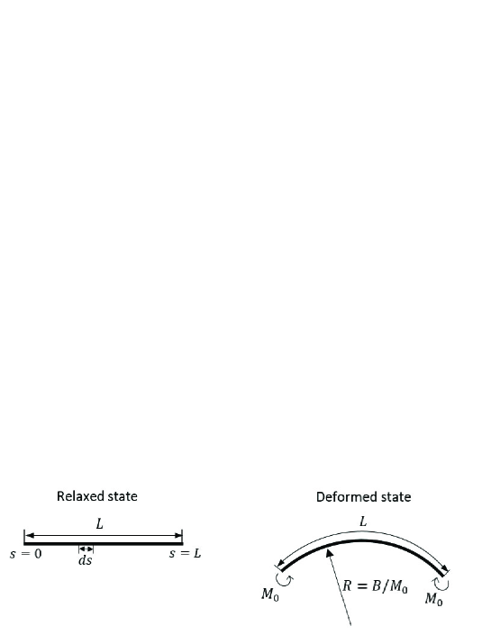
Figure 2: A flat thin sheet is deformed into a cylinder of constant radius without stretching of its midplane. This deformation is obtained for the extensible elastica by applying bending moments, $M_{0}$, on the sheet edges or by imposing $d\phi/ds$ at the boundaries.

To apply the formulation to this simple problem we should reduce the 2D energy, Eq. (15), to 1D. Consider a radial cut of a $\theta$-independent deformation as a planar compatible filament ($\Phi(r)=1$). Identify $r\rightarrow s$, where $s\in[0,L]$ is the undeformed arclength along the filament, and $\phi^{r}(r)\rightarrow\phi(s)$, the angle between the tangent to the filament and the flat reference plane. We then have $\phi_{rr}^{2}\rightarrow\phi_{ss}^{2}=(d\phi/ds)^{2}$, $\epsilon_{rr}\rightarrow\epsilon_{ss}$, and $\phi_{\theta\theta}=\epsilon_{\theta\theta}=0$. Substitution of these relations in Eq. (15) gives,

$$E_{\rm 1D}=E_{s}+E_{b}=\int_{0}^{L}\left[\frac{Y}{2}\epsilon_{ss}^{2}+\frac{B}{2}\left(\frac{d\phi}{ds}\right)^{2}\right]ds.$$ (22)

This functional coincides with the energy of an extensible elastic filament in a planar deformation as given by the theory of extensible elastica Reissner (1972); Magnusson et al. (2001); Oshri and Diamant (2016); Humer (2013).

Alternatively, we could reduce the sheet into a filament through an azimuthal cut along a narrow annulus of large radius $\rho$, in which case $d\theta\rightarrow ds$, $\phi_{\theta\theta}^{2}\rightarrow\phi_{ss}=(d\phi/(\Phi ds))^{2}$, and $\phi_{rr}=\epsilon_{rr}=0$. We then obtain

$$E_{\rm 1D}=E_{s}+E_{b}=\int_{0}^{L^{\prime}}\left[\frac{Y}{2}\epsilon_{ss}^{2}+\frac{B}{2}\left(\frac{d\phi}{\Phi ds}\right)^{2}\right]\Phi ds.$$ (23)

The parameter $s$ now runs between $0$ and $L^{\prime}$, such that $L=\int_{0}^{L^{\prime}}\Phi ds$ is the total relaxed length. In addition, $\epsilon_{ss}$ now measures the in-plane strain with respect to the prescribed metric. The energy of Eq. (23) is the extension of the extensible elastica theory to the case of a nontrivial reference metric.

Returning to the ordinary elastica, we note that Eq. (22) can be derived from a discrete model of springs and joints Oshri and Diamant (2016) while enforcing from the outset the decoupling between the stretching and bending contributions (Libai and Simmonds, 1988, p. 77). In Eq. (22) this decoupling is manifest in the independence of $E_{s}$ on $\phi$, $\frac{\delta E_{s}}{\delta\phi}=0$, while $E_{b}$ is independent of $\epsilon_{ss}$, $\frac{\delta E_{b}}{\delta\epsilon_{ss}}=0$. In the absence of boundary axial forces, the equations of equilibrium are obtained from minimization of Eq. (22). Defining the in-plane stress (acting to only locally stretch the filament) and bending moment (acting only to change its local angle) as,

$$\sigma_{ss}\equiv\frac{\delta E_{\rm 1D}}{\delta\epsilon_{ss}}=Y\epsilon_{ss},$$ (24a)

$$M_{ss}\equiv\frac{\delta E_{\rm 1D}}{\delta\left(\frac{d\phi}{ds}\right)}=B\frac{d\phi}{ds},$$ (24b)

those equations of equilibrium are,

$$\sigma_{ss}=0,$$ (25a)

$$\frac{dM_{ss}}{ds}=0.$$ (25b)

When a constant moment, $M_{0}$, is applied at the boundaries (Fig. 2), Eqs. (24a)–(25b) yield $\epsilon_{ss}=0$ and $\phi(s)=\phi(0)+(M_{0}/B)s$. This solution corresponds to a circular arc of radius $B/M_{0}$ and total length $L$. Alternatively, if we impose $(d\phi/ds)|_{s=0}=c$, we get $\phi(s)=\phi(0)+cs$, corresponding to a circular arc of radius $1/c$. The energy of this configuration is $E_{\rm 1D}=(B/2)c^{2}L$.

The strain-free cylindrical shape is preserved also in the more complicated case of a nonuniform reference metric, Eq. (23). Variation of this energy with respect to $\epsilon_{ss}$ and $\phi$ gives, as before, Eqs. (25), where the in-plane stress is given again by Eq. (24a). The bending moment is modified to,

$$M_{ss}=\frac{\delta E_{\rm 1D}}{\delta\left(\frac{1}{\Phi}\frac{d\phi}{ds}\right)}=\frac{B}{\Phi}\frac{d\phi}{ds},$$ (26)

which replaces Eq. (24b). The in-plane strain (with respect to the reference metric) vanishes. When we apply a moment $M_{0}$ at the boundaries, or impose $(d\phi/(\Phi ds))|_{s=0}=c$, we find again a strain-free cylindrical shape with radius $B/M_{0}$, or $1/c$.

We now show that the ESK functional gives a different result. We specialize Eq. (I) to the case of a compatible sheet under uniaxial deformation. Since the deformation has zero Gaussian curvature, we set $\bar{g}_{ss}=1$ and, from Eq. (2), obtain $a_{ss}=1+2\tilde{\epsilon}_{ss}$. In addition, we have $\sqrt{|\bar{g}|}dA\rightarrow ds$, $t\mathcal{A}^{ssss}\rightarrow Y$, and $\frac{t^{3}}{12}\mathcal{A}^{ssss}\rightarrow\ B$. Substituting these relations in Eq. (I) gives

$$\text{ESK:}\ \ \ E_{\rm 1D}=\int_{0}^{L}\left(\frac{Y}{2}\tilde{\epsilon}_{ss}^{2}+\frac{B}{2}b_{ss}^{2}\right)ds.$$ (27)

The relations between the variables appearing in the ESK Eq. (27) and the ones in Eq. (22) are $\tilde{\epsilon}_{ss}=\epsilon_{ss}(1+\epsilon_{ss}/2)$, and $b_{ss}=\partial_{s}(\sqrt{a_{ss}}\hat{{\bf t}})\cdot\hat{{\bf n}}=(1+2\tilde{\epsilon}_{ss})^{1/2}\frac{d\phi}{ds}$.

Naively, if we set the variations of the energy (27) with respect to $\tilde{\epsilon}_{ss}$ and $b_{ss}$ to zero, we will get the same result as above, i.e., a strain-free circular configuration with $\tilde{\epsilon}_{ss}=0$, $b_{ss}=(d\phi/ds)_{s=0}=c$, and energy $E_{\rm 1D}=(B/2)c^{2}L$. Thus, the coupling between $\tilde{\epsilon}_{ss}$ and $d\phi/ds$ appearing in $b_{ss}=(1+2\tilde{\epsilon}_{ss})^{1/2}\frac{d\phi}{ds}$ would not have an effect on the configuration. However, the correct minimization is with respect to the filament’s trajectory ${\bf f}(s)$. As shown in Appendix A, this is equivalent to the minimization with respect to $\epsilon_{ss}$ and $\phi$. In terms of these variables, Eq. (27) becomes

$$\text{ESK:}\ \ \ E_{\rm 1D}=\int_{0}^{L}\left[\frac{Y}{2}[\epsilon_{ss}(1+\epsilon_{ss}/2)]^{2}+\frac{B}{2}[1+2\epsilon_{ss}(1+\epsilon_{ss}/2)\left(\frac{d\phi}{ds}\right)^{2}\right]ds.$$ (28)

The bending contribution to this energy depends on $\epsilon_{ss}$, which results in a strained configuration under the boundary conditions given above. Specifically, minimization of the energy in Eq. (28) with respect to $\epsilon_{ss}$ and $\phi$, under the boundary condition $(d\phi/ds)_{s=0}=c$, yields a circular arc, $\phi(s)=\phi(0)+cs$, which nonetheless contains non-zero strain, $\epsilon_{ss}=\sqrt{1-2Bc^{2}/Y}-1$. The energy of this configuration is $E_{\rm 1D}=(B/2)c^{2}L[1-(B/Y)c^{2}]$, slightly deviating from the energy of the extensible elastica obtained above.

Two comments should be added concerning the difference between the two models. (a) As demonstrated by the case of a geometrical boundary condition on $d\phi/ds$, the difference does not arise from different definitions of the boundary bending moment. (This remains correct if we impose the condition on the apparent curvature, $[d\phi/d(1+\epsilon_{ss})s]_{s=0}$.) (b) In Ref. Efrati et al. (2009a) a term proportional to $\tilde{\epsilon}_{ss}(d\phi/ds)^{2}$ was neglected in the final step. Clearly, its inclusion merely changes the numerical coefficient in the second term of Eq. (28).

In summary, unlike the formulation of Sec. II, the ESK model does not strictly reduce to the extensible elastica. Under uniaxial bending at the boundaries it produces a small in-plane strain, while our formulation and the extensible elastica predict a strain-free cylindrical shape. The discrepancy is small and vanishes in the incompressible limit of $B/Y\rightarrow 0$. Moreover, the correction terms are of order $(B/Y)c^{2}\sim(tc)^{2}$, which must always be small in any elasticity theory of sheets of finite thickness. Nevertheless, the effect of the coupling between stress and bending moments goes beyond this simple 1D example and profoundly affects the structure of the theory, as will be shown in the following sections.

IV Exact solutions for planar deformations of incompatible sheets

We now demonstrate the advantage of the alternative formulation in simple examples of flat configurations. In the flat state the bending energy is zero and the equation of equilibrium is obtained by minimizing the stretching energy alone. To do so we first set $\zeta=0$ in Eqs. (11),

$$\epsilon_{rr}=\partial_{r}u_{r},$$ (29a)

$$\epsilon_{\theta\theta}=\frac{r}{\Phi}-1+\frac{u_{r}}{\Phi},$$ (29b)

and then substitute Eqs. (29) in (16), obtaining,

$$E_{s}=\frac{1}{2}\int_{0}^{R}\int_{0}^{2\pi}\left[\sigma_{rr}\partial_{r}u_{r}+\sigma_{\theta\theta}\left(\frac{r}{\Phi}-1+\frac{u_{r}}{\Phi}\right)\right]\Phi d\theta dr.$$ (30)

Minimization of $E_{s}$ with respect to $u_{r}$ gives the equation of equilibrium,

$$\partial_{r}(\Phi\sigma_{rr})-\sigma_{\theta\theta}=0,$$ (31)

which expresses balance of forces in the radial direction (see Fig. 3). Substituting the in-plane strains, Eqs. (29), in the stress components, Eqs. (17), and then in (31), we obtain the equation of equilibrium in terms of $u_{r}$ alone,

$$\Phi\partial_{r}(\Phi\partial_{r}u_{r})-u_{r}=r-\Phi-\nu\Phi(1-\partial_{r}\Phi).$$ (32)

This second-order equation for $u_{r}$ is supplemented by two boundary conditions: vanishing stress at the free edge, $\left.\sigma_{rr}\right|_{r=R}=0$ and vanishing displacement at the origin. The resulting conditions are

$$\left[\Phi\partial_{r}u_{r}+\nu u_{r}+\nu\left(r-\Phi\right)\right]_{r=R}=0,$$ (33a)

$$\left.u_{r}\right|_{r=0}=0.$$ (33b)

Importantly, unlike earlier analysis of the same problem Efrati et al. (2009b), Eqs. (32) and (33) are linear and therefore solvable. To demonstrate this key advantage we now derive exact solutions of Eq. (32) for three types of reference metrics: flat, elliptic, and hyperbolic (see Fig. 4).

Figure 3: Radial force balance on an infinitesimal element of a flat sheet (Timoshenko, 1970, p. 65). At the point $P$ we have contributions from the two radial stresses, $(\sigma_{rr})_{1}\Phi d\theta$ and $-(\sigma_{rr})_{3}\Phi d\theta$, and from the two azimuthal stresses $-(\sigma_{\theta\theta})_{2}dr\sin(d\theta/2)$ and $-(\sigma_{\theta\theta})_{4}dr\sin(d\theta/2)$. Balancing these terms gives Eq. (31).

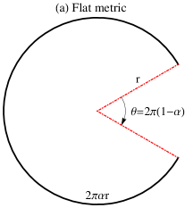
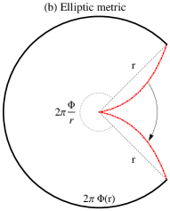
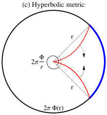
Figure 4: Layouts of the three considered reference metrics. (a) Flat metric, Eq. (34). When the two radii (dash-dotted red lines) are held together, the rest length of concentric circles on the closed disc become $2\pi\alpha r<2\pi r$. (b) Elliptic metric, Eq. (40). Gluing together the two curved dash-dotted red lines creates a frustrated disc, where concentric circles have rest length of $2\pi\Phi(r)<2\pi r$. (c) Hyperbolic metric, Eq. (47). In this panel dashing represents unseen lines; concentric circles have rest length $2\pi\Phi(r)>2\pi r$, causing pieces of the disc to be placed in the relaxed configuration one over the other (marked in blue). Attaching together the lower (hidden) red-dashed line with the upper solid red line results in a disc with a hyperbolic metric.

In the following subsections we compare the results obtained from analytical solutions of our model for the different reference metrics with those obtained from the ESK nonlinear equations. To assure a meaningful comparison we examine the following: (a) the radial displacement $u_{r}$, which is an unambiguous experimental observable; (b) the stress components obtained by variation of the energy with respect to the strain $\epsilon$ (not the metric-based one, $\tilde{\epsilon}$) for both models. In the Supplemental Material D we elaborate on the relations between these stress tensors in the two theories.

IV.1 Flat metric

A flat reference metric is given by,

$$\Phi(r)=\alpha r,$$ (34)

where $\alpha<1$. Substituting Eq. (34) in (32) and (33a) gives,

$$\alpha^{2}r\partial_{r}(r\partial_{r}u_{r})-u_{r}=(1-\alpha)(1-\nu\alpha)r,$$ (35a)

$$\left[\alpha r\partial_{r}u_{r}+\nu u_{r}+\nu(1-\alpha)r\right]_{r=R}=0.$$ (35b)

Equation (35a) replaces the nonlinear Eq. (10) of Ref. Efrati et al. (2009b) which could be solved only numerically. The solution to Eq. (35a) is given by,

$$u_{r}(r)=A_{0}r^{1/\alpha}+B_{0}r^{-1/\alpha}-\frac{1-\alpha\nu}{1+\alpha}r,$$ (36)

where $A_{0}$ and $B_{0}$ are constants to be determined by boundary conditions. The vanishing displacement at the disc center, Eq. (33b), is satisfied for $B_{0}=0$. The value of $A_{0}$ is determined by the second boundary condition, (35b). This gives,

$$u_{r}(r)=-\frac{1-\alpha\nu}{1+\alpha}\left[1-\frac{(1-\nu)\alpha}{1-\alpha\nu}\left(\frac{r}{R}\right)^{\frac{1}{\alpha}-1}\right]r.$$ (37)

Substituting Eq. (37) in Eqs. (29) and then in Eqs. (17), we obtain the radial and azimuthal stress components,

$$\sigma_{rr}(r)=-\frac{Et}{1+\alpha}\left[1-\left(\frac{r}{R}\right)^{\frac{1}{\alpha}-1}\right],$$ (38a)

$$\sigma_{\theta\theta}(r)=-\frac{Et}{1+\alpha}\left[\alpha-\left(\frac{r}{R}\right)^{\frac{1}{\alpha}-1}\right].$$ (38b)

Note that the stress components do not depend on $\nu$. Note also that the azimuthal stress becomes positive at $r_{cr}=\alpha^{\alpha/(1-\alpha)}R$, whereas the radial one is always negative. The problem can be solved for other boundary conditions, e.g., for an annulus with inner radius $R_{i}$ and outer radius $R_{o}$, and with free boundary conditions at its two rims. The solution reads,

$$u_{r}=\frac{\alpha(1-\nu)}{1+\alpha}\left[\frac{1-\rho^{\frac{1}{\alpha}+1}}{1-\rho^{2/\alpha}}\left(\frac{r}{R_{o}}\right)^{\frac{1}{\alpha}-1}-\frac{1+\nu}{1-\nu}\,\frac{1-\rho^{\frac{1}{\alpha}-1}}{1-\rho^{2/\alpha}}\left(\frac{R_{i}}{r}\right)^{\frac{1}{\alpha}+1}-\frac{1-\nu\alpha}{\alpha(1-\nu)}\right]r,$$ (39a)

$$\sigma_{rr}=-\frac{Et}{1+\alpha}\left[1-\frac{1-\rho^{\frac{1}{\alpha}+1}}{1-\rho^{2/\alpha}}\left(\frac{r}{R_{o}}\right)^{\frac{1}{\alpha}-1}-\frac{1-\rho^{\frac{1}{\alpha}-1}}{1-\rho^{2/\alpha}}\left(\frac{R_{i}}{r}\right)^{\frac{1}{\alpha}+1}\right],$$ (39b)

$$\sigma_{\theta\theta}=-\frac{Et}{1+\alpha}\left[\alpha-\frac{1-\rho^{\frac{1}{\alpha}+1}}{1-\rho^{2/\alpha}}\left(\frac{r}{R_{o}}\right)^{\frac{1}{\alpha}-1}+\frac{1-\rho^{\frac{1}{\alpha}-1}}{1-\rho^{2/\alpha}}\left(\frac{R_{i}}{r}\right)^{\frac{1}{\alpha}+1}\right],$$ (39c)

where $\rho\equiv R_{i}/R_{o}$. In Fig. 5 we compare the exact analytical solution for the radial displacement, Eq. (39a), with the numerical solution of the formalism given in Ref. Efrati et al. (2009b). The two theories converge to the same solution as $\alpha\rightarrow 1$. However, away from this nearly Euclidean regime there are significant differences in the resultant displacements. Since the displacement is an unambiguous observable, these differences underline the fact that the two formulations are not equivalent. Figure 6 presents a similar comparison of the plane stresses obtained from the two theories.

Figure 5: Comparison between the exact solution for the radial displacement (Eq. (39a); black, solid line) and the numerical solution of Eq. (10) in Ref. Efrati et al. (2009b) (dashed, blue line) for a flat reference metric. We consider an annulus with inner and outer radii $R_{i}=0.1$ and $R_{o}=1.1$. In accordance with the example in Ref. Efrati et al. (2009b), we use $\nu=0$.

Figure 6: Comparison between the exact plane-stress solutions (Eqs. (39), black solid line) and the numerical solution of Eq. (10) in Ref. Efrati et al. (2009b) (dashed blue line) for a flat reference metric. Parameters are as in Fig. 5.

IV.2 Elliptic metric

An elliptic reference metric is given by,

$$\Phi(r)=\frac{1}{\sqrt{K}}\sin(\sqrt{K}r),$$ (40)

where $K$ is a constant positive reference Gaussian curvature. Substituting Eq. (40) in Eqs. (32) and (33a) gives,

$$\sin(r)\partial_{r}(\sin(r)\partial_{r}u_{r})-u_{r}=r-\sin(r)-\nu\sin(r)(1-\cos(r)),$$ (41a)

$$\left[\sin(r)\partial_{r}u_{r}+\nu u_{r}+\nu(r-\sin(r))\right]_{r=R}=0,$$ (41b)

where we have rescaled the lengths $r$ and $u_{r}$ by $K^{-1/2}$. The following expression is verified to be the general solution by direct substitution in Eq. (41a),

$$u_{r}(r)=A_{0}\tan(r/2)+B_{0}\cot(r/2)-r-2(1+\nu)\cot(r/2)\ln[\cos(r/2)].$$ (42)

We set $B_{0}=0$ to satisfy the vanishing displacement at the disc center, Eq. (33b), and determine $A_{0}$ by the boundary condition (41b), obtaining,

$$u_{r}(r)=-r-2(1-\nu)\ln[\cos(R/2)]\cot^{2}(R/2)\left(1+\frac{1+\nu}{1-\nu}\frac{\cot^{2}(r/2)}{\cot^{2}(R/2)}\frac{\ln[\cos(r/2)]}{\ln[\cos(R/2)]}\right)\tan(r/2).$$ (43)

Note that the solution diverges for $r=r_{n}=n\pi$ where $n$ is a positive integer. At such points the reference metric, Eq. (40), vanishes, i.e., these divegencies correspond to unphysical cases where the rest length shrinks to zero. Substituting Eq. (43) in Eqs. (17), we obtain the distributed stress on the disc,

$$\sigma_{rr}(r)=-Et\left(1-\frac{\cot^{2}(r/2)}{\cot^{2}(R/2)}\frac{\ln[\cos(r/2)]}{\ln[\cos(R/2)]}\right)\frac{\ln[\cos(R/2)]\cot^{2}(R/2)}{\cos^{2}(r/2)},$$ (44a)

$$\sigma_{\theta\theta}(r)=-Et\left(1+\frac{\ln[\cos(r/2)]}{\sin^{2}(r/2)}+\cot^{2}(R/2)\frac{\ln[\cos(R/2)]}{\cos^{2}(r/2)}\right).$$ (44b)

Once again, the solution is independent of the Poisson ratio.

In order to compare our exact solution to the numerical one obtained in Ref. Efrati et al. (2009b), we also derive the displacement and the planar stress in an annulus with free boundary conditions. In this case the constants $A_{0}$ and $B_{0}$ in Eq. (42) are

$$A_{0}=\frac{4(1-\nu)}{\cos(R_{i})-\cos(R_{o})}\cos^{2}(R_{i}/2)\cos^{2}(R_{o}/2)\left(\ln[\cos(R_{i}/2)]-\ln[\cos(R_{o}/2)]\right),$$ (45a)

$$B_{0}=\frac{1+\nu}{\cos(R_{i})-\cos(R_{o})}\left[(1+\cos(R_{i}))(1-\cos(R_{o}))\ln[\cos(R_{i}/2)]-(1-\cos(R_{i}))(1+\cos(R_{o}))\ln[\cos(R_{o}/2)]\right],$$

and the stress components become

$$\sigma_{rr} = -2Et\left[1+\left(1-\frac{\cos(R_{i})-\cos(R_{o})}{\cos(r)-\cos(R_{o})}\frac{\cos^{2}(r/2)}{\cos^{2}(R_{i}/2)}\frac{\ln[\cos(r/2)]}{\ln[\cos(R_{i}/2)]}\right)\frac{1+\cos(R_{i})}{1+\cos(R_{o})}\frac{\cos(r)-\cos(R_{o})}{\cos(R_{i})-\cos(r)}\frac{\ln[\cos(R_{i}/2)]}{\ln[\cos(R_{o}/2)]}\right]$$ (46a)

$$\times \frac{1+\cos(R_{o})}{\sin^{2}(r)}\frac{\cos(R_{i})-\cos(r)}{\cos(R_{i})-\cos(R_{o})}\ln[\cos(R_{o}/2)],$$

$$\sigma_{\theta\theta} = -Et\left[1+\frac{\ln[\cos(r/2)]}{\sin^{2}(r/2)}+4\left(1-\frac{\cos^{2}(R_{i}/2)}{\cos^{2}(R_{o}/2)}\frac{1-\cos(R_{o})\cos(r)}{1-\cos(R_{i})\cos(r)}\frac{\ln[\cos(R_{i}/2)]}{\ln[\cos(R_{o}/2)]}\right)\right.$$ (46b)

$$\times \left.\frac{\cos^{2}(R_{o}/2)}{\sin^{2}(r)}\frac{1-\cos(R_{i})\cos(r)}{\cos(R_{i})-\cos(R_{o})}\ln[\cos(R_{o}/2)]\right].$$

In Fig. 7 we compare the radial displacement obtained from this exact solution, Eqs. (42) and (45), to the numerical solution of Eq. (10) in Ref. Efrati et al. (2009b). In addition, Fig. 8 compares the radial and azimuthal stress components of the two models. The two solutions converge for a narrow annulus and differ significantly as the annulus becomes wider. (Note that increasing $R_{o}$ is equivalent to increasing $K$.)

Figure 7: The exact solution for the radial displacement (Eqs. (42) and (45); black solid line) is plotted alongside the numerical solution of Eq. (10) in Ref. Efrati et al. (2009b) (dashed blue line) for an elliptic reference metric. We consider an annulus with a normalized inner radius $R_{i}=0.1$, $\nu=0$, and two different values of $R_{o}$ as indicated.

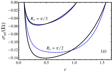
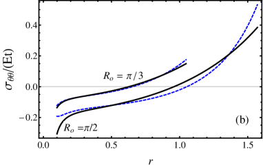
Figure 8: Comparison between the exact plane-stress solutions, Eqs. (46) (black solid line), and the numerical results based on Ref. Efrati et al. (2009b) (dashed blue line) for an elliptic reference metric. Parameters as in Fig. 7.

IV.3 Hyperbolic metric

A hyperbolic reference metric is given by,

$$\Phi(r)=\frac{1}{\sqrt{K}}\sinh(\sqrt{K}r).$$ (47)

The equation of equilibrium and the boundary condition are obtained by substituting Eq. (47) in Eq. (32) and (33a),

$$\sinh(r)\partial_{r}(\sinh(r)\partial_{r}u_{r})-u_{r}=r-\sinh(r)+\nu\sinh(r)(1-\cosh(r)),$$ (48a)

$$\left[\sinh(r)\partial_{r}u_{r}+\nu u_{r}+\nu(r-\sinh(r))=0\right]_{r=R},$$ (48b)

where again we have rescaled $r$ and $u_{r}$ by $K^{-1/2}$. Since Eq. (48a) is obtained from (41a) by a Wick transformation,

$$r\rightarrow ir,\ \ \ \ u_{r}\rightarrow iu_{r},$$ (49)

we immediately obtain from Eqs. (43) and (44) the solution,

$$u_{r}(r)=-r+2(1-\nu)\coth^{2}(R/2)\ln[\cosh(R/2)]\left(1+\frac{1+\nu}{1-\nu}\,\frac{\coth^{2}(r/2)}{\coth^{2}(R/2)}\frac{\ln[\cosh(r/2)]}{\ln[\cosh(R/2)]}\right)\tanh(r/2),$$ (50a)

$$\sigma_{rr}(r)=Et\left(1-\frac{\coth^{2}(r/2)}{\coth^{2}(R/2)}\frac{\ln[\cosh(r/2)]}{\ln[\cosh(R/2)]}\right)\frac{\ln[\cosh(R/2)]\coth^{2}(R/2)}{\cosh^{2}(r/2)},$$ (50b)

$$\sigma_{\theta\theta}(r)=-Et\left(1-\frac{\ln[\cosh(r/2)]}{\sinh^{2}(r/2)}-\cosh^{2}(R/2)\frac{\ln[\cosh(R/2)]}{\cosh^{2}(r/2)}\right).$$ (50c)

It is readily verified that this solution satisfies the boundary condition (48b).

Similarly, the radial displacement and the stress distribution in an annulus with hyperbolic reference metric is obtained from Eqs. (46) via a Wick transformation, Eq. (49). In Figs. 9 and 10 we compare these solutions to the one obtained in Ref. Efrati et al. (2009b).

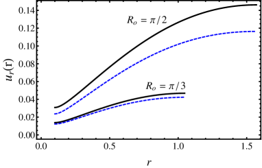
Figure 9: The exact solution for the radial displacement (black solid line) is plotted alongside the numerical solution of Eq. (10) in Ref. Efrati et al. (2009b) (dashed blue line) for a hyperbolic reference metric. We consider an annulus with inner normalized radius $R_{i}=0.1$, $\nu=0$, and two different values of $R_{o}$ as indicated.

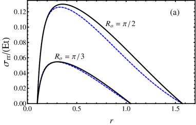
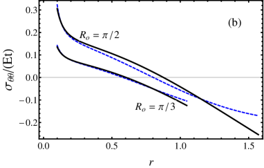
Figure 10: The exact radial and azimuthal plane-stress solutions for a flat annulus with a hyperbolic reference metric (solid black line) are compared with the numerical solution of Eq. (10) in Ref. Efrati et al. (2009b) (dashed blue line). Parameters are as in Fig. 9.

V Stability criterion for isometric immersions

An isometric immersion refers to a strain-free configuration, $\epsilon_{\alpha\beta}\equiv 0$, leading to $E_{s}=0$. It is obviously the minimizer of the elastic energy for $B=0$. In this section we do not directly seek the minimizer of the total energy, Eq. (15), but check whether the isometric immersion happens to be a minimizer also for $B>0$. Since this configuration already minimizes $E_{s}$, we need to check only whether it also minimizes $E_{b}$. Note, however, that there are two different routes for such minimization: (a) set $\epsilon_{\alpha\beta}=0$ in $E_{b}$ and then minimize with respect to curvature alone; (b) minimize $E_{b}$ with respect to both strain and curvature and only then set the strain to zero, which is the appropriate route. It is straightforward to show that in our model the two routes are equivalent. This is because the strain appears only quadratically in the energy (see, for example, Eq. (22)) and, therefore, setting the strain to zero, either before or after minimization, eliminates the same terms. However, in the ESK model the additional coupling term in the bending energy is linear in the strain (compare, for example, to Eq. (27)), leading to different results of the two routes. Hence, we conclude that the two theories should give the same results in case (a) but may differ in the appropriate minimization, case (b).

For a given reference metric of the form of Eq. (3), i.e., for a given $\Phi(r)$, the requirement of vanishing strain uniquely determines the configuration of the sheet up to rigid transformations. Indeed, setting Eqs. (11) to zero, we obtain,

$$u_{r}(r)=\Phi-r,$$ (51a)

$$\partial_{r}\zeta=\sqrt{1-(\partial_{r}\Phi)^{2}}.$$ (51b)

We can now check whether this configuration satisfies local mechanical equilibrium of bending moments.

We substitute in Eq. (18) $\phi_{rr}=\partial_{r}\phi^{r}$ and $\phi_{\theta\theta}=\sin\phi^{r}/\Phi$ (see Fig. 1(a)),

$$E_{b}=\frac{1}{2}\int_{0}^{R}\int_{0}^{2\pi}\left[M_{rr}\partial_{r}\phi^{r}+M_{\theta\theta}\sin\phi^{r}/\Phi\right]\Phi d\theta dr,$$ (52)

and minimize with respect to $\phi^{r}$,

$$\partial_{r}(\Phi M_{rr})-\cos\phi^{r}M_{\theta\theta}=0,$$ (53a)

$$\left.M_{rr}\right|_{r=R}=0.$$ (53b)

(As has been done for the uniaxial bending case (Appendix A), one can show here as well that this minimization is equivalent to the appropriate one with respect to the spatial configuration; see Supplemental Material D.) Equation (53a) expresses balance of moments on an infinitesimal sheet element in the radial direction Libai and Simmonds (1988); Simmonds and Libai (1987). The boundary condition, Eq. (53b), imposes the vanishing of radial bending moment at the free edge.

Our aim now is to check whether the displacements given by Eqs. (51) also satisfy Eqs. (53). To this end we first express $\phi_{rr}$ and $\phi_{\theta\theta}$ in terms of $\Phi(r)$ using Eqs. (13) and (51),

$$\phi_{rr}=-\partial_{rr}\Phi/\sqrt{1-(\partial_{r}\Phi)^{2}},$$ (54a)

$$\phi_{\theta\theta}=\sqrt{1-(\partial_{r}\Phi)^{2}}/\Phi.$$ (54b)

In addition, we have (see the relation between $\phi_{\theta\theta}$ and the angle $\phi^{r}$ in Fig. 1(a) and its caption),

$$\cos\phi^{r}=\partial_{r}\Phi.$$ (55)

Substituting Eqs. (54) in Eqs. (19), and the result, along with Eq. (55), in Eqs. (53), we obtain an equation and a boundary condition for $\Phi(r)$ alone,

$$\partial_{r}(\Phi\partial_{rr}\Phi/\sqrt{1-(\partial_{r}\Phi)^{2}})+\partial_{r}\Phi\sqrt{1-(\partial_{r}\Phi)^{2}}/\Phi=0,$$ (56a)

$$\left[\partial_{rr}\Phi/\sqrt{1-(\partial_{r}\Phi)^{2}}-\nu\sqrt{1-(\partial_{r}\Phi)^{2}}/\Phi\right]_{r=R}=0.$$ (56b)

Equations (56) are a self-consistency condition for the reference metric, which must be satisfied for the isometric immersion to be an equilibrium configuration of the total energy. (It should be stressed that, if a certain isometric immersion does not satisfy this condition, it can still become the equilibrium configuration asymptotically, in the limit of vanishing $B/Y$ Lewicka, Marta and Reza Pakzad, Mohammad (2011).)

The displacements, Eqs. (51), and the bulk equilibrium equation, Eq. (56a), do not depend on $\nu$. Hence, any solution but the trivial flat configuration, $\Phi(r)=r$, will violate, in general, the boundary condition (56b), which does depend on $\nu$ explicitly. In Ref. Efrati et al. (2009b) it was shown that such boundary conditions may be taken care of by boundary layers. Thus, up to a small correction at the boundary (which vanishes in the limit of zero thickness), an isometry that satisfies the bulk condition, Eq. (56a), may be in mechanical equilibrium even if the boundary condition (56b) is not satisfied.

Let us now check the stability condition, Eq. (56a), for the examples of flat and elliptic reference metrics. In the case of a hyperbolic one, Eq. (47), the isometric immersion is not a surface of revolution Klein et al. (2011), and therefore lies outside the scope of this work. (Substituting Eq. (47) in the height function, Eq. (51b), produces an imaginary result.)

Considering a flat reference metric, $\Phi(r)=\alpha r$, we immediately find that the self-consistency condition, Eq. (56a), is violated, and conclude that any isometric immersion of this metric will be unstable for $B>0$. The isometric immersion of the flat metric is a cone with an opening angle $\mathcal{\vartheta}=2\tan^{-1}(\alpha/\sqrt{1-\alpha^{2}})$,

$${\bf f}(r,\theta)=r\left[\alpha{\bf\hat{r}}+\sqrt{1-\alpha^{2}}{\bf\hat{z}}\right].$$ (57)

Note again that this does not preclude the possibility that the actual minimizer approaches a cone asymptotically for a vanishingly small $B/Y$ Lewicka, Marta and Reza Pakzad, Mohammad (2011).

In the example of an elliptic reference metric we substitute Eq. (40) in (56a) and find that the self-consistency condition is satisfied in the bulk. The isometric immersion of an elliptic reference metric is a spherical cap of radius $1/\sqrt{K}$,

$${\bf f}(r,\theta)=\frac{1}{\sqrt{K}}\left(\sin(\sqrt{K}r)\hat{{\bf r}}+\cos(\sqrt{K}r)\hat{{\bf z}}\right).$$ (58)

When we substitute this configuration in the formalism of Ref. Efrati et al. (2009a) (the first of Eqs. (3.10) in Ref. Efrati et al. (2009a)), we find that it does not satisfy balance of normal forces (see Supplemental Material D). This procedure corresponds to route (b) described above, i.e., substitution of the isometric immersion in the full equations of equilibrium rather than eliminating the strain from the beginning. Thus, as anticipated above, the two theories disagree. A spherical cap satisfies our stability condition but is found to be unstable for $B>0$ by the ESK theory. (Recall that the two theories do coincide if one wrongly follows the other route in the ESK model.) The spherical cap configuration of a sheet with elliptic reference metric was found to be stable in experiments Klein et al. (2011). We note that the criterion at the boundary, Eq. (56b), is not satisfied by the elliptic $\Phi(r)$. This can be mended by a thin boundary layer of width $\propto t^{1/2}$ Efrati et al. (2009b). In Appendix B we give an alternative, more complete derivation of this result within the FvK approximation.

In Appendix C we add a similar stability criterion for two examples of surfaces of revolution whose reference metric is slightly more general than the ones assumed so far.

VI Discussion

We have presented an alternative formulation for the elasticity of incompatible thin sheets, which is restricted to axisymmetric deformations. This formulation and the existing ESK theory Efrati et al. (2009b) are not equivalent. The lack of equivalence has been demonstrated in three systems — the existence or absence of in-plane strain in a uniaxially bent sheet (Sec. III); the strains forming in flat incompatible sheets (Sec. IV, see Figs. 5 and 7); and the stability of the spherical-cap isometry for a sheet with an elliptic reference metric (Sec. V).

The key ingredient that sets the two models apart is a coupling between stretching and bending, which appears in the ESK model upon dimensional reduction, and is removed in the present formulation by using distance deviations, rather than metric deviations, to define strain. (Recall, for example, Eq. (22) vs. Eq. (27).) Let us pinpoint the stage at which this difference emerges. If the derivation of Eqs. (5)–(12) is repeated for the Green-St. Venant strain, Eq. (1), then Eqs. (12) are replaced by $\tilde{\epsilon}_{rr}^{\star}=\tilde{\epsilon}_{rr}-2x_{3}b_{rr}+x_{3}^{2}c_{rr}$, and $\tilde{\epsilon}_{\theta\theta}^{\star}=\tilde{\epsilon}_{\theta\theta}-2x_{3}b_{\theta\theta}/\Phi^{2}+x_{3}^{2}c_{\theta\theta}/\Phi^{2}$. The different dependence on the $x_{3}$ coordinate perpendicular to the mid-surface, inevitably leads to additional terms upon integration of the energy over $x_{3}$.

Quantitatively, the differences caused by the coupling term are small and indeed may lie outside the strict limits of the infinitesimal-strain theory. They seem negligible experimentally. The removal of this term, however, leads to a much simpler analysis, as demonstrated by the exact solutions in Sec. IV. (A similar observation was made in the context of beam theory Irschik and Gerstmayr (2009).) Since, at least for the problems considered in this manuscript, the differences can be neglected, there is freedom, and clear benefit, in choosing a more tractable formulation when it is available.

The two models become equivalent in the incompressible limit, $B/Y=0$. The problems treated in Secs. III and V reveal an essential difference in the way the two models depart from this limit. Both problems — the uniaxially bent sheet and the sheet with elliptic reference metric — possess a strain-free configuration (isometric immersion) as the energy minimizer for $B/Y=0$. According to the ESK model this configuration ceases to be the minimizer for an arbtirarily small but finite $B/Y$; according to the model presented here it remains the energy minimizer to leading order in $B/Y$. In other words, as $B/Y$ tends to zero, the equilibrium configuration reaches the isometry with nonzero slope in the former, and with zero slope in the latter. In a sheet made of a 3D material both $Y$ and $B$ emanate from the same elastic modulus. Then, it may well be that a stretching-bending coupling exists even in the absence of Gaussian curvature, leading with decreasing thickness to the “nonzero slope” behavior. In a genuinely 2D sheet, such as a monomolecular layer or a 2D polymer network, $Y$ and $B$ can be independent (e.g., arising from the rigidities of bonds and bond angles, respectively). In such cases, for example, it may well be that stretching and bending should be decoupled, leading to the “zero slope” case — i.e., an isometry (no stretched bonds) remaining the energy minimizer for $B/Y>0$ (finite joint rigidity). These delicate issues might be checked in discrete simulations. While being conceptually interesting, they may have (at least according to the problems considered here) little practical significance.

The exact solutions presented in Sec. IV for the strains and stresses in flat incompatible sheets can be used as the base solutions for a perturbative (near-threshold) treatment of buckling instabilities in these systems, which can then be studied experimentally. Our formulation can be applied to additional examples beyond those addressed in Secs. IV and V, where the reference metric is axisymmetric. An interesting problem, for instance, might be the case of a highly localized (delta-function) $\Phi(r)$. In addition, the theory might be useful for analyzing stress fields around two-dimensional defects Moshe et al. (2015a, b).

The most important extension of this work, however, would be to obtain a similarly tractable formulation for sheets of any two-dimensional deformation. The discussion above suggests two possible routes. One is to generalize the formulation presented in Sec. II beyond axisymmetric deformations. The other is to modify the ESK energy functional such that the two choices of strain measures lead to equivalent theories.

Appendix A Consistent energy minimization for a uniaxially deformed sheet

In this Appendix we show that minimization of $E_{\rm 1D}$ with respect to $\epsilon_{ss}$ and $\phi$ yields equations of equilibrium which are identical to the ones obtained by the appropriate minimization with respect to the spatial configuration, ${\bf f}(s)$.

We first define the perturbed configuration, $\tilde{\bf f}(s)$, by

$$\tilde{\bf f}(s)={\bf f}(s)+\delta{\bf f}(s)={\bf f}(s)+\psi_{t}(s){\bf\hat{t}}+\psi_{n}(s){\bf\hat{n}},$$ (59)

where $\{{\bf\hat{t}}(s),{\bf\hat{n}}(s)\}$ are the unit vectors tangent and normal to the sheet along the deformation axis, and $\psi_{t}$ and $\psi_{n}$ are arbitrary perturbation functions. Equivalently (up to a shift of the origin), we can represent the configuration by $d{\bf f}/ds$, i.e., $d\tilde{\bf f}/ds=d{\bf f}/ds+d\delta{\bf f}/ds$. Then, the variation of the energy is written as

$$\delta E_{\rm 1D}=\int({\cal E}_{t}{\bf\hat{t}}+{\cal E}_{n}{\bf\hat{n}})\cdot\frac{d\delta{\bf f}}{ds}ds,$$ (60)

where ${\cal E}_{t}$ and ${\cal E}_{n}$ are some functions of $\epsilon_{ss}$ and $\phi$ yet to be determined. We wish to relate the variation $d\delta{\bf f}/ds$ with the variations $\delta\epsilon_{ss}$ and $\delta\phi$.

The vectors $\{{\bf\hat{t}}(s),{\bf\hat{n}}(s)\}$ satisfy the Frenet-Serret formulas Lipschutz (1969),

$$\frac{d{\bf\hat{t}}}{ds}=(1+\epsilon_{ss})\kappa{\bf\hat{n}}=\frac{d\phi}{ds}{\bf\hat{n}},$$ (61a)

$$\frac{d{\bf\hat{n}}}{ds}=-(1+\epsilon_{ss})\kappa{\bf\hat{t}}=-\frac{d\phi}{ds}{\bf\hat{t}},$$ (61b)

where $\kappa=d\phi/d\hat{s}$ is the curvature and $\hat{s}$ is the arclength of the deformed configuration, $d\hat{s}/ds=1+\epsilon_{ss}$. With the help of Eqs. (61), differentiating $\delta{\bf f}$ of Eq. (59) with respect to $s$ gives

$$\frac{d\delta{\bf f}}{ds}=\left(\frac{d\psi_{t}}{ds}-\frac{d\phi}{ds}\psi_{n}\right){\bf\hat{t}}+\left(\frac{d\psi_{n}}{ds}+\frac{d\phi}{ds}\psi_{t}\right){\bf\hat{n}}.$$ (62)

Next, we examine the in-plane variation $\delta\epsilon_{ss}$ to leading order in the perturbation functions,

$$\delta\epsilon_{ss}=\left|\frac{d{\bf\tilde{f}}}{ds}\right|-\left|\frac{d{\bf f}}{ds}\right|\simeq\frac{d\psi_{t}}{ds}-\frac{d\phi}{ds}\psi_{n},$$ (63)

To do the same for the $\delta\phi$ we start by writing $\cos\phi={\bf\hat{t}}\cdot{\bf\hat{x}}$, where ${\bf\hat{x}}$ is a constant unit vector along the horizontal direction. Upon variation we have, $-\sin\phi\delta\phi=\delta{\bf\hat{t}}\cdot{\bf\hat{x}}$. In turn, the variation of the tangent vector is given by,

$$\delta{\bf\hat{t}}=\frac{d{\bf\tilde{f}}/ds}{|d{\bf\tilde{f}}/ds|}-\frac{d{\bf f}/ds}{|d{\bf f}/ds|}\simeq\frac{1}{1+\epsilon_{ss}}\left(\frac{d\psi_{n}}{ds}+\frac{d\phi}{ds}\psi_{t}\right){\bf\hat{n}},$$ (64)

and, since ${\bf\hat{n}}\cdot{\bf\hat{x}}=-\sin\phi$, we get

$$(1+\epsilon_{ss})\delta\phi=\frac{d\psi_{n}}{ds}+\frac{d\phi}{ds}\psi_{t}.$$ (65)

Collecting the results for $\delta\epsilon_{ss}$ and $\delta\phi$ (Eqs. (63) and (65)) and substituting in Eq. (62), we obtain the desired relation,

$$\frac{d\delta{\bf f}}{ds}=\delta\epsilon_{ss}{\bf\hat{t}}+(1+\epsilon_{ss})\delta\phi{\bf\hat{n}}.$$ (66)

This proves that the variation with respect to the spatial configuration is equivalent to the variation with respect to $\delta\epsilon_{ss}$ and $\delta\phi$.

We can proceed to rewrite the variation of the energy, Eq. (60), as

$$\delta E_{\rm 1D}=\int\left[{\cal E}_{t}\delta\epsilon_{ss}+(1+\epsilon_{ss}){\cal E}_{n}\delta\phi\right]ds.$$ (67)

The straightforward way to get the equations of equilibrium is to set this functional to zero for arbitrary $\delta\epsilon_{ss}$ and $\delta\phi$, i.e., ${\cal E}_{t}=0$ and ${\cal E}_{n}=0$. This is what has been done in Sec. III, where

$${\cal E}_{t}=Y\epsilon_{ss}=\sigma_{ss}=0,$$ (68a)

$${\cal E}_{n}=-\frac{B}{1+\epsilon_{ss}}\frac{d^{2}\phi}{ds^{2}}=-\frac{dM_{ss}}{d\hat{s}}=0.$$ (68b)

(See Eqs. (24) and (25).)

Alternatively, we can rewrite the energy variation, Eq. (60), in terms of $\delta{\bf f}$ rather than $d\delta{\bf f}/ds$, using intergration by parts. This yields the equations of equilibrium in the different form,

$$\frac{d{\cal E}_{t}}{ds}-\frac{d\phi}{ds}{\cal E}_{n}=0,$$ (69a)

$$\frac{d{\cal E}_{n}}{ds}+\frac{d\phi}{ds}{\cal E}_{t}=0.$$ (69b)

Subtituting Eqs. (68), this gives

$$\frac{d\sigma_{ss}}{d\hat{s}}-\kappa\sigma_{sn}=0,$$ (70a)

$$\frac{d\sigma_{sn}}{d\hat{s}}+\kappa\sigma_{ss}=0,$$ (70b)

where $\sigma_{sn}=-dM_{ss}/d\hat{s}$ is the normal force at a cross section (Love, 1927, p. 387).

The difference between the two equivalent sets of equilibrium equations is explained in Fig. 11. While Eqs. (68) represent balance of forces and moments across a finite segment of the sheet, Eqs. (70) represent the balance for an infinitesimal segment.

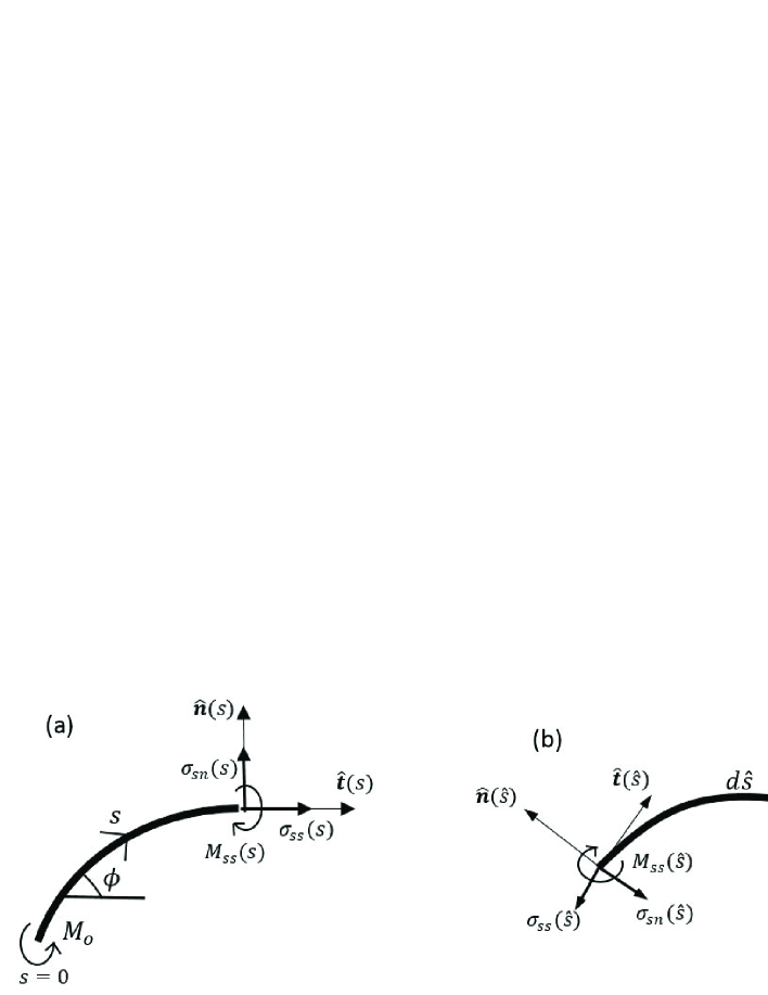
Figure 11: (a) Schematic force balance on a finite sheet segment. A bending moment, $M_{o}$, applied at the boundary, is balanced by the reaction forces, $\sigma_{ss}$ and $\sigma_{sn}$, and the reaction bending moment, $M_{ss}$. Under these conditions $\sigma_{ss}=\sigma_{sn}=0$ and $M_{ss}=M_{o}$, consistently with Eqs. (68). (b) Schematic force balance on an infinitesimal sheet segment of length $d\hat{s}$. Balance of forces in the tangential direction, ${\bf\hat{t}}(\hat{s})$, is given by, $-\sigma_{ss}(\hat{s})+\sigma_{ss}(\hat{s}+d\hat{s}){\bf\hat{t}}(\hat{s}+d\hat{s})\cdot{\bf\hat{t}}(\hat{s})+\sigma_{sn}(\hat{s}+d\hat{s}){\bf\hat{n}}(\hat{s}+d\hat{s})\cdot{\bf\hat{t}}(\hat{s})=0$. Expanding this equation to leading order in the differential $d\hat{s}$ (using Eqs. (61)) we obtain $d\sigma_{ss}/d\hat{s}-\kappa\sigma_{sn}=0$. Similarly, force balance in the normal direction and balance of bending moments gives: $d\sigma_{sn}/d\hat{s}+\kappa\sigma_{ss}=0$ and $dM_{ss}/d\hat{s}+\sigma_{ns}=0$, consistently with Eqs. (70).

Appendix B Boundary layer in a sheet with elliptic reference metric

In this Appendix we show that the energy of the isometric spherical cap, Eq. (58), is reduced when a boundary layer is formed (i) near the outer radius of a complete disc, and (ii) near the outer and inner radii of an annulus. The existence of these boundary layers and the scaling of their width with the thickness $t$ were found in Ref. Efrati et al. (2009b). Here we derive these results based on a variational Ansatz within the FvK approximation, thus obtaining full expressions including prefactors.

Considering the elliptic reference metric, Eq. (40), and employing the small-slope approximation, we obtain for the in-plane strains, Eqs. (11),

$$\epsilon_{rr}\simeq\partial_{r}u_{r}+\frac{1}{2}(\partial_{r}\zeta)^{2},$$ (71a)

$$\epsilon_{\theta\theta}\simeq\frac{Kr^{2}}{6}+\frac{u_{r}}{r}.$$ (71b)

For the isometric immersion these strains vanish, yielding the height function $\zeta_{iso}\simeq\sqrt{K}r^{2}/2$. The total energy of the spherical cap is obtained by substituting this function in Eq. (21), giving,

$$E_{iso}=\pi(1+\nu)(KR^{2})B.$$ (72)

Let us try to reduce the total energy below $E_{iso}$ through the following variational Ansatz:

$$\zeta(r)=\zeta_{iso}+\zeta_{bl}=\frac{\sqrt{K}r^{2}}{2}-\frac{(1+\nu)}{\alpha(\alpha+\nu-1)}\sqrt{K}R^{2}\left(\frac{r}{R}\right)^{\alpha},$$ (73)

where $\alpha$ serves as a variational parameter. The coefficient of the second term in Eq. (73) has been chosen so as to satisfy the boundary condition of zero radial bending moment at the outer radius, $\left.M_{rr}\right|_{r=R}\simeq B\left[\partial_{rr}\zeta+\frac{\nu}{r}\partial_{r}\zeta\right]_{r=R}=0$. When $\alpha\gg 1$ the additional term is negligible everywhere except close to the edge, as expected from a boundary layer. As shown below, the minimizing configuration has $\alpha\sim t^{-1/2}$.

Since our Ansatz, Eq. (73), is not an isometry, it contains in-plane stress. To calculate this stress we first minimize the stretching energy, Eq. (16), with respect to $u_{r}$. In the FvK approximation the resulting equation reads,

$$\partial_{r}(r\sigma_{rr})-\sigma_{\theta\theta}=0.$$ (74)

Substituting, Eq. (73) in the strains, Eqs. (71), and then in the stress-strain relations, Eqs. (17), we obtain from Eq. (74),

$$r\partial_{r}(r\partial_{r}u_{r})-u_{r}=-\frac{4}{3}Kr^{3}+(1+\nu)\frac{\alpha-\nu+1}{\alpha+\nu-1}KR^{3}\left(\frac{r}{R}\right)^{\alpha+1}+\frac{1}{2}(1+\nu)^{2}\frac{\nu-2\alpha+1}{(\alpha+\nu-1)^{2}}KR^{3}\left(\frac{r}{R}\right)^{2\alpha-1}.$$ (75)

Two boundary conditions are necessary: one is a vanishing stress at the free edge, $\left.\sigma_{rr}\right|_{r=R}=0$, and the other is a vanishing displacement at the origin, $\left.u_{r}\right|_{r=0}=0$. The solution of Eq. (75) subject to these conditions is,

$$u_{r}(r)=A_{0}r-\frac{K}{6}r^{3}+\frac{(1+\nu)(\alpha-\nu+1)}{\alpha(\alpha+2)(\alpha+\nu-1)}KR^{3}\left(\frac{r}{R}\right)^{\alpha+1}+\frac{1}{8}\frac{(1+\nu)^{2}(\nu-2\alpha+1)}{\alpha(\alpha-1)(\alpha+\nu-1)^{2}}KR^{3}\left(\frac{r}{R}\right)^{2\alpha-1},$$ (76)

where $A_{0}$ is determined by the first boundary condition.

Substituting $u_{r}$ and $\zeta$ from Eqs. (73) and (76), in Eqs. (16) and (21), and expanding to leading order in $1/\alpha$, gives,

$$E\simeq\frac{\pi}{2}YR^{2}(KR^{2})^{2}(1-\nu)(1+\nu)^{3}\alpha^{-5}+\pi(1+\nu)(KR^{2})B-\frac{3\pi}{2}(1+\nu)^{2}(KR^{2})B\alpha^{-1},$$ (77)

where the first term comes from stretching and the last two are bending contributions. Minimization of Eq. (77) with respect to $\alpha$ yields,

$$\alpha=(5/3)^{1/4}(1-\nu^{2})^{1/4}(KR^{2})^{1/4}(YR^{2}/B)^{1/4}=(20)^{1/4}(1-\nu^{2})^{1/4}(KR^{2})^{1/4}(t/R)^{-1/2}.$$ (78)

Substituting this result in Eq. (77) we finally obtain,

$$E\simeq E_{iso}-\frac{6\pi}{5}\left(\frac{3}{5}\right)^{1/4}\frac{(1+\nu)^{2}}{(1-\nu^{2})^{1/4}}(KR^{2})^{3/4}\left(\frac{B}{YR^{2}}\right)^{1/4}B,$$ (79)

where $E_{iso}$ is given by Eq. (72). Thus, the energy of the isometric immersion is reduced by the introduction of a boundary layer. The reduction scales as $t^{7/2}$ whereas $E_{iso}\sim t^{3}$. In the limit of small thickness we can write $\zeta_{bl}(r)\simeq-\frac{(1+\nu)\sqrt{K}R^{2}}{\alpha^{2}}e^{-(R-r)/w}$ with the width of the boundary layer being,

$$w=R/\alpha=(20)^{-1/4}(1-\nu^{2})^{-1/4}(KR^{2})^{-1/4}(t/R)^{1/2}R.$$ (80)

This derivation can straightforwardly be extended to the more general case of an annulus with inner radius $R_{i}$ and outer radius $R_{o}$. In this case the energy of the isometric immersion, $\zeta_{iso}$, is given by,

$$E_{iso}=\pi(1+\nu)K(R_{o}^{2}-R_{i}^{2})B.$$ (81)

This energy can be reduced below $E_{iso}$ if two boundary layers are formed near the outer and inner radii, as indicated by the following Ansatz,

$$\zeta(r)=\zeta_{iso}+\zeta_{bl}=\frac{\sqrt{K}r^{2}}{2}+A_{o}\left(\frac{r}{R_{o}}\right)^{\alpha}+B_{o}\left(\frac{R_{i}}{r}\right)^{\alpha}.$$ (82)

As in the case of a disc, $A_{o}$ and $B_{o}$ are chosen such that the radial bending moment is zero at the two boundaries, $\left.M_{rr}\right|_{r=R_{i},R_{o}}=0$. This gives,

$$A_{o}=-\sqrt{K}R_{o}^{2}\frac{1+\nu}{\alpha(\alpha+\nu-1)}\frac{1-\rho^{\alpha+2}}{1-\rho^{2\alpha}},$$ (83a)

$$B_{o}=-\sqrt{K}R_{i}^{2}\frac{1+\nu}{\alpha(\alpha-\nu+1)}\frac{1-\rho^{\alpha-2}}{1-\rho^{2\alpha}},$$ (83b)

where $\rho\equiv R_{i}/R_{o}$.

Following the same route as in Eqs. (74)-(76), we find after expansion in powers of $\alpha^{-1}$ and assuming $\rho^{\alpha}\rightarrow 0$ that the total energy of the annulus is given by,

$$E\simeq\frac{\pi}{2}YR_{o}^{2}(KR_{o}^{2})^{2}\left(1+\rho^{6}\right)(1-\nu)(1+\nu)^{3}\alpha^{-5}+\pi(1+\nu)K(R_{o}^{2}-R_{i}^{2})B-\frac{3\pi}{2}(1+\nu)^{2}(KR_{o}^{2})\left(1+\rho^{2}\right)B\alpha^{-1}.$$

Minimization of this energy with respect to $\alpha$ gives,

$$\alpha = (5/3)^{1/4}(1-\nu^{2})^{1/4}\left(\frac{1+\rho^{6}}{1+\rho^{2}}\right)^{1/4}(KR_{o}^{2})^{1/4}\left(\frac{YR_{o}^{2}}{B}\right)^{1/4}$$ (85)

$$= (20)^{1/4}(1-\nu^{2})^{1/4}\left(\frac{1+\rho^{6}}{1+\rho^{2}}\right)^{1/4}(KR_{o}^{2})^{1/4}\left(\frac{t}{R_{o}}\right)^{-1/2}.$$

Note that in the limit of $\rho\rightarrow 0$ this result coincides with Eq. (78). Substituting Eq. (85) back in the energy, Eq. (B), we obtain,

$$E\simeq E_{iso}-\frac{6\pi}{5}\left(\frac{3}{5}\right)^{1/4}\frac{(1+\nu)^{2}}{(1-\nu^{2})^{1/4}}(KR_{o}^{2})^{3/4}\frac{\left(1+\rho^{2}\right)^{5/4}}{\left(1+\rho^{6}\right)^{1/4}}\left(\frac{B}{YR_{o}^{2}}\right)^{1/4}B,$$ (86)

where $E_{iso}$ is given by Eq. (81). Thus, the introduction of two boundary layers, at the inner and outer radii of the annulus, reduce the energy of an isometric immersion.

Appendix C Stability criterion for isometric immersions with negative Gaussian curvature

In this appendix we extend the theory presented in Sec. II to surfaces of revolution, [see Eq. (4)], whose reference metric is given by,

$$\bar{g}_{\alpha\beta}=\begin{pmatrix}\bar{g}_{r}^{2}&0\\ 0&\bar{g}_{\theta}^{2}\end{pmatrix}\ \ \ ,\ \ \ ds^{2}=\bar{g}_{r}^{2}(r)dr^{2}+\bar{g}_{\theta}^{2}(r)d\theta^{2}.$$ (87)

Our aim is to derive a self-consistent stability criterion, similar to Eqs. (56), for isometric immersions with constant negative Gaussian curvature Gemmer and Venkataramani (2011).

Following Sec. II it is straightforward to show that the energy functional, Eq. (15), is modified into,

$$E=\frac{Y}{2}\int_{0}^{R}\int_{0}^{2\pi}\left[\epsilon_{rr}^{2}+\epsilon_{\theta\theta}^{2}+2\nu\epsilon_{rr}\epsilon_{\theta\theta}\right]\bar{g}_{r}\bar{g}_{\theta}d\theta dr+\frac{B}{2}\int_{0}^{R}\int_{0}^{2\pi}\left[\phi_{rr}^{2}+\phi_{\theta\theta}^{2}+2\nu\phi_{rr}\phi_{\theta\theta}\right]\bar{g}_{r}\bar{g}_{\theta}d\theta dr,$$ (88)

where the in-plane strains are given by,

$$\epsilon_{rr}=\sqrt{a_{rr}}/\bar{g}_{r}-1=\sqrt{(1+\partial_{r}u_{r})^{2}+(\partial_{r}\zeta)^{2}}/\bar{g}_{r}-1,$$ (89a)

$$\epsilon_{\theta\theta}=\sqrt{a_{\theta\theta}}/\bar{g}_{\theta}-1=(r+u_{r})/\bar{g}_{\theta}-1,$$ (89b)

and the “bending-strains”, are given by,

$$\phi_{rr}=\sqrt{c_{rr}}/\bar{g}_{r}=\frac{1}{\bar{g}_{r}}\frac{(1+\partial_{r}u_{r})\partial_{rr}\zeta-\partial_{rr}u_{r}\partial_{r}\zeta}{(1+\partial_{r}u_{r})^{2}+(\partial_{r}\zeta)^{2}}=\partial_{r}\phi^{r}/\bar{g}_{r},$$ (90a)

$$\phi_{\theta\theta}=\sqrt{c_{\theta\theta}}/\bar{g}_{\theta}=\frac{1}{\bar{g}_{\theta}}\frac{\partial_{r}\zeta}{\sqrt{(1+\partial_{r}u_{r})^{2}+(\partial_{r}\zeta)^{2}}}=\sin\phi^{r}/\bar{g}_{\theta}.$$ (90b)

Setting Eqs. (89) to zero, we obtain the displacement corresponding to the isometric immersion of Eq. (87),

$$u_{r}=\bar{g}_{\theta}-r,$$ (91a)

$$\partial_{r}\zeta=\sqrt{\bar{g}_{r}^{2}-(\partial_{r}\bar{g}_{\theta})^{2}}.$$ (91b)

Following the analysis in Sec. V, we minimize the bending energy,

$$E_{b}=\frac{1}{2}\int_{0}^{R}\int_{0}^{2\pi}\left[M_{rr}\partial_{r}\phi^{r}/\bar{g}_{r}+M_{\theta\theta}\sin\phi^{r}/\bar{g}_{\theta}\right]\bar{g}_{r}\bar{g}_{\theta}d\theta dr,$$

with respect to $\phi^{r}$ to obtain the balance of bending moments. This gives,

$$\partial_{r}(\bar{g}_{\theta}M_{rr})-\bar{g}_{r}\cos\phi^{r}M_{\theta\theta}=0.$$ (92)

where $M_{\alpha\beta}$ are given by Eqs. (19) and $\phi_{\alpha\beta}$ are given by Eqs. (90).

Substituting the displacements of Eqs. (91) in the “bending strains”, Eqs. (90), we obtain,

$$\phi_{rr}=\left(\partial_{r}\bar{g}_{\theta}\partial_{r}\sqrt{\bar{g}_{r}^{2}-(\partial_{r}\bar{g}_{\theta})^{2}}-\partial_{rr}\bar{g}_{\theta}\sqrt{\bar{g}_{r}^{2}-(\partial_{r}\bar{g}_{\theta})^{2}}\right)/\bar{g}_{r}^{3},$$ (93a)

$$\phi_{\theta\theta}=\sqrt{\bar{g}_{r}^{2}-(\partial_{r}\bar{g}_{\theta})^{2}}/(\bar{g}_{r}\bar{g}_{\theta}).$$ (93b)

In addition, using Eq. (90b), we have that,

$$\cos\phi^{r}=\partial_{r}\bar{g}_{\theta}/\bar{g}_{r}.$$ (94)

Substituting Eqs. (93) in (19) and then, along with Eq. (94), in (92) we finally obtain the self-consistency condition,

$$\partial_{r}\left(\bar{g}_{\theta}\left(\partial_{r}\bar{g}_{\theta}\partial_{r}\sqrt{\bar{g}_{r}^{2}-(\partial_{r}\bar{g}_{\theta})^{2}}-\partial_{rr}\bar{g}_{\theta}\sqrt{\bar{g}_{r}^{2}-(\partial_{r}\bar{g}_{\theta})^{2}}\right)/\bar{g}_{r}^{3}\right)-\partial_{r}\bar{g}_{\theta}\sqrt{\bar{g}_{r}^{2}-(\partial_{r}\bar{g}_{\theta})^{2}}/(\bar{g}_{r}\bar{g}_{\theta})=0.$$ (95)

It is now straightforward to verify that a pseudosphere, $\bar{g}_{r}=\tanh r$ and $\bar{g}_{\theta}=1/\cosh r$, and hyperboloid of revolution, $\bar{g}_{r}=b\ \text{sn}(r,b)$ and $\bar{g}_{\theta}=\text{dn}(r,b)$ (sn and dn denoting the Jacobi elliptic functions Abramowitz and Stegun (1965)), both do not satisfy Eq. (95). Thus, both are mechanically unstable. As in the case of the cone, we note that these conclusions do not rule out the possibility that the objects approach these shapes in the limit $t\rightarrow 0$.

Appendix D Supplementary material:
Comparison between thin sheet theories based on model-independent force-balance equations

As has been demonstrated in the main text by several examples, the ESK model and the present one produce different equations of equilibrium and different equilibrium configurations. Yet, obviously, both models describe balance of forces and torques. Therefore, using an appropriate representation, both should result in identical (albeit not equivalent) equations of equilibrium. Thus the lack of equivalence would be confined to the relations between stress and deformation (the constitutive relations), and we would get an instructive comparison of the stress and torque under similar loading conditions in the two models. Such a representation is the goal of this Supplemental Material.

While the present model is based on the Biot strain measure, Eq. (10), the ESK theory Efrati et al. (2009a) is based on the second Piola-Kirchhoff strain, Eq. (1). As a result, our equilibrium equations, Eqs. (32) and (53a), manifestly differ from the ones obtained in Ref. Efrati et al. (2009a), Eq. (3.10) in that paper.

To derive the conditions of force and torque balance we first define the co-moving coordinate system $\{{\bf\hat{t}}_{r},{\bf\hat{t}}_{\theta},{\bf\hat{n}}\}$, where ${\bf\hat{t}}_{\alpha}=\partial_{\alpha}{\bf f}/|\partial_{\alpha}{\bf f}|$ are two in-plane unit vectors and ${\bf\hat{n}}$ is the unit normal, given the spatial configuration ${\bf f}(r,\theta)$. Second, we cut an infinitesimal patch of the surface, whose borders lie along lines of constant coordinates (Gol’Denveizer, 1961, p. 24), and balance the force and torque vectors applied on its edges. This gives (Gol’Denveizer, 1961, p. 29),

$$0=\partial_{r}(\Phi{\bf F}_{r})+\partial_{\theta}{\bf F}_{\theta},$$ (96a)

$$0=\partial_{r}(\Phi{\bf M}_{r})+\partial_{\theta}{\bf M}_{\theta}-\Phi\partial_{r}{\bf f}\times{\bf F}_{r}-\partial_{\theta}{\bf f}\times{\bf F}_{\theta},$$ (96b)

where ${\bf F}_{\alpha}$ and ${\bf M}_{\alpha}$ are the forces and bending moments per undeformed unit length along the directions $\alpha=r,\theta$. Lastly, we resolve the components of these vectors projected on our triad basis,

$${\bf F}_{\alpha}=\sigma_{\alpha r}{\bf\hat{t}}_{r}+\sigma_{\alpha\theta}{\bf\hat{t}}_{\theta}+\sigma_{\alpha 3}{\bf\hat{n}},$$ (97a)

$${\bf M}_{\alpha}={\bf\hat{n}}\times(M_{\alpha r}{\bf\hat{t}}_{r}+M_{\alpha\theta}{\bf\hat{t}}_{\theta}).$$ (97b)

Note the delicate point, crucial for the sake of this section, that the tensors $\sigma_{\alpha\beta}$ and $M_{\alpha\beta}$ here correspond to the actual forces and torques, i.e., the fluxes of linear and angular momenta. As such, they do not depend on the choice of model; unlike Eqs. (17) and (19) in the main text, we do not relate them at this moment to a certain definition of strain. In other words, they are not necessarily equal to the variation of the energy of the chosen model with respect to the strain and curvature of that model. Similarly, the configuration is represented in these equations through the model-independent spatial triad $\{{\bf\hat{t}}_{r},{\bf\hat{t}}_{\theta},{\bf\hat{n}}\}$.

For axisymmetric deformations, Eq. (4), we always have $\sigma_{r\theta}=M_{r\theta}=0$, and Eqs. (96) and (97) form a system of five differential equations for the eight unknowns, $\{\sigma_{\alpha\alpha},\sigma_{\alpha 3},M_{\alpha\alpha},u_{r},\zeta\}$, where the configuration is now represented by the displacements $u_{r}$ and $\zeta$, obtainable from $\{{\bf\hat{t}}_{r},{\bf\hat{t}}_{\theta},{\bf\hat{n}}\}$. Thus, to have a closure we must derive constitutive relations between the stress and torque components and the actual deformation.

The definition of mechanical energy, as well, does not depend on the choice of model. It is the sum of two terms: (i) The work done by in-plane forces to displace the sheet from its rest state to the given configuration (not displacement squared), and (ii) the work done by bending moments to change the out-of-plane angles from their rest values. For clarity of the expressions that follow, it is helpful to represent the displacements equivalently by in-plane stretching fields, $\gamma_{\alpha\alpha}\equiv\sqrt{a_{\alpha\alpha}/\bar{g}_{\alpha\alpha}}$, and out-of-plane bending fields, $\bar{g}_{\alpha\alpha}\phi_{\alpha\alpha}\equiv b_{\alpha\alpha}/\gamma_{\alpha\alpha}$ (where $\alpha=r,\theta$, and the mixed terms vanish by axisymmetry). The variation of the energy is given then by the infinitesimal work,

$$\delta E=\int_{0}^{R}\int_{0}^{2\pi}\left(\sigma_{\alpha\beta}\delta\gamma_{\alpha\beta}+M_{\alpha\beta}\delta\phi_{\alpha\beta}\right)\Phi drd\theta.$$ (98)

We note that Eq. (98) is the 2D extension of the so-called principle of virtual work Irschik and Gerstmayr (2009); Reissner (1972). In addition, similar to our proof in Appendix A it can be shown that $\delta\gamma_{\alpha\beta}$ and $\delta\phi_{\alpha\beta}$ are consistent with minimization of the energy with respect to the configuration. These infinitesimals are proportional to the 1D variations, $\delta\epsilon_{ss}$ and $\delta\phi$, considered in Sec. III.

If we now consider the energy functional of each model, express it in terms of the actual deformation fields $\gamma_{\alpha\alpha}$ and $\phi_{\alpha\alpha}$, and take the variation with respect to these fields, we will get the constitutive relations for the actual stresses and bending moments, as arising from each model.

The energy functional of the present model (Eq. (15)) is rewritten in terms of the deformation fields as

$$E_{\rm 2D}= \frac{Y}{2}\int_{0}^{R}\int_{0}^{2\pi}\left[(\gamma_{rr}-1)^{2}+(\gamma_{\theta\theta}-1)^{2}+2\nu(\gamma_{rr}-1)(\gamma_{\theta\theta}-1)\right]\Phi d\theta dr$$ (99)

$$+\frac{B}{2}\int_{0}^{R}\int_{0}^{2\pi}\left[\phi_{rr}^{2}+\phi_{\theta\theta}^{2}+2\nu\phi_{rr}\phi_{\theta\theta}\right]\Phi d\theta dr.$$

Variations with respect to $\gamma_{\alpha\alpha}$ and $\phi_{\alpha\alpha}$ give

$$\sigma_{rr}=Y\left[(\gamma_{rr}-1)+\nu(\gamma_{\theta\theta}-1)\right],$$ (100a)

$$\sigma_{\theta\theta}=Y\left[(\gamma_{\theta\theta}-1)+\nu(\gamma_{rr}-1)\right],$$ (100b)

$$M_{rr}=B\left(\phi_{rr}+\nu\phi_{\theta\theta}\right),$$ (100c)

$$M_{\theta\theta}=B\left(\phi_{\theta\theta}+\nu\phi_{rr}\right).$$ (100d)

The energy functional of the ESK model is obtained by specializing Eq. (I) to the axisymmetric case and re-expressing it in terms of the deformation fields, yielding

$$\mbox{ESK:}\ \ \ E_{\rm 2D} = \frac{Y}{8}\int_{0}^{R}\int_{0}^{2\pi}\left[(\gamma_{rr}^{2}-1)^{2}+(\gamma_{\theta\theta}^{2}-1)^{2}+2\nu(\gamma_{rr}^{2}-1)(\gamma_{\theta\theta}^{2}-1)\right]\Phi d\theta dr$$ (101)

$$+\frac{B}{2}\int_{0}^{R}\int_{0}^{2\pi}\left[(\gamma_{rr}\phi_{rr})^{2}+(\gamma_{\theta\theta}\phi_{\theta\theta})^{2}+2\nu(\gamma_{rr}\phi_{rr})(\gamma_{\theta\theta}\phi_{\theta\theta})\right]\Phi d\theta dr.$$

Variations of this energy with respect to $\gamma_{\alpha\alpha}$ and $\phi_{\alpha\alpha}$ give

ESK: $$\sigma_{rr}=\frac{Y}{2}\gamma_{rr}\left[(\gamma_{rr}^{2}-1)+\nu(\gamma_{\theta\theta}^{2}-1)\right]+B\phi_{rr}\left(\gamma_{rr}\phi_{rr}+\nu\gamma_{\theta\theta}\phi_{\theta\theta}\right),$$ (102d)

$$\sigma_{\theta\theta}=\frac{Y}{2}\gamma_{\theta\theta}\left[(\gamma_{\theta\theta}^{2}-1)+\nu(\gamma_{rr}^{2}-1)\right]+B\phi_{\theta\theta}\left(\gamma_{\theta\theta}\phi_{\theta\theta}+\nu\gamma_{rr}\phi_{rr}\right),$$

$$M_{rr}=B\gamma_{rr}\left(\gamma_{rr}\phi_{rr}+\nu\gamma_{\theta\theta}\phi_{\theta\theta}\right),$$

$$M_{\theta\theta}=B\gamma_{\theta\theta}\left(\gamma_{\theta\theta}\phi_{\theta\theta}+\nu\gamma_{rr}\phi_{rr}\right).$$

The comparison between the constitutive relations in Eqs. (100) and Eqs. (102) underlines once again the difference between the two models. While the former relations are linear, the latter are nonlinear; while in the former $\sigma_{\alpha\alpha}$ depend only on $\gamma_{\alpha\alpha}$ and $M_{\alpha\alpha}$ depend only on $\phi_{\alpha\alpha}$, in the latter there are mixed terms.

A natural question then is how the actual stresses given by these relations correspond to the ones obtained by variation of the energy with respect to the strain as it is defined in each model. In the present model they are identical; compare Eqs. (100) to Eqs. (17) and (19). This is because the relation between $\gamma_{\alpha\alpha}$ and the strain $\epsilon_{\alpha\alpha}$ used in this model is linear; hence, $\delta\epsilon_{\alpha\alpha}=\delta\gamma_{\alpha\alpha}$. The stress and moments tensors, $s^{\alpha\alpha}$ and $m^{\alpha\alpha}$, which were defined in Ref. Efrati et al. (2009a) differ from the actual ones, Eqs. (102). The stress, $s^{\alpha\alpha}$, is based on variation of the energy with respect to the strain $\tilde{\epsilon}_{\alpha\alpha}$ and the bending moment, $m^{\alpha\alpha}$, is based on variation of the energy with respect to the second fundamental form $b_{\alpha\alpha}$. The two sets of stresses and bending moments, $\{\sigma_{\alpha\alpha},M_{\alpha\alpha}\}$ from Eqs. (102) and $\{s^{\alpha\alpha},m^{\alpha\alpha}\}$ are inter-related according to

$$\mbox{ESK:}\ \ \ \ \sigma_{rr} = \gamma_{rr}s^{rr}+\phi_{rr}m^{rr},$$ (103a)

$$\sigma_{\theta\theta} = \Phi^{2}(\gamma_{\theta\theta}s^{\theta\theta}+\phi_{\theta\theta}m^{\theta\theta}),$$ (103b)

$$M_{rr} = \gamma_{rr}m^{rr},$$ (103c)

$$M_{\theta\theta} = \Phi^{2}\gamma_{\theta\theta}m^{\theta\theta}.$$ (103d)

In summary, the equations of equilibrium (96b) and (97b) are model-independent and, in particular, common to the two models compared here. They become different only once the different constitutive relations, either (100) or (102), are substituted in them. Upon this substitution, one obtains the equations of equilibrium, predicted by the respective model from minimization of its respective energy over spatial configurations ${\bf f}$. We now demonstrate it in two examples.

D.1 Flat deformations

In the case of flat deformations, $\zeta=0$, we have from both models , $M_{\alpha\alpha}=0$. Substituting this result in the torque balance equation (96b), we get also that the normal stresses vanishing, $\sigma_{\alpha 3}=0$. In addition, for the case of planar axisymmetric deformations Eq. (96a) is automatically satisfied in the tangential and normal directions. Thus, the only non-vanishing equation is the balance of forces in the radial direction, which reads,

$$\partial_{r}(\Phi\sigma_{rr})-\sigma_{\theta\theta}=0.$$ (104)

This recovers Eq. (31) of the main text. Since we have not yet used a constitutive relation, this equation holds also in the ESK model.

Substituting in Eq. (104) the constitutive relations of the present model, Eqs. (100a) and (100b), we recover the linear equilibrium equation of the main text, Eq. (32). Repeating the same using the ESK constitutive relations (102d) and (102d), we obtain

$$\partial_{r}\left(\Phi\gamma_{rr}s^{rr}\right)-\Phi^{2}\gamma_{\theta\theta}s^{\theta\theta}=0,$$ (105)

where the ESK stresses of Eq. (103) have been used. Finally, introducing the Christoffel symbols, $\Gamma_{rr}^{r}=\partial_{r}\gamma_{rr}/\gamma_{rr}$ and $\Gamma_{\theta\theta}^{r}=-\Phi\gamma_{\theta\theta}/\gamma_{rr}$, we recover Eq. (7) of Ref. Efrati et al. (2009b),

$$\frac{1}{\Phi}\partial_{r}(\Phi s^{rr})+\Gamma_{rr}^{r}s^{rr}+\Gamma_{\theta\theta}^{r}s^{\theta\theta}=0.$$ (106)

This equation exhibits the covariant form of the ESK theory. At the same time it has the disadvantage of being nonlinear in the displacement, $u_{r}$, compared to the present model’s linear Eq. (32).

D.2 Normal force balance in an isometric immersion

As a second example we return to the issue addressed in Sec. V, i.e., the balance of normal forces in the spherical-cap isometry of a sheet with elliptic reference metric. Once again, we apply the different sets of constitutive relations of the two models to the model-independent equations of equilibrium, and compare the results. In the ESK case this procedure recovers, here based on force balance, the first of Eqs. (3.10) in Ref. Efrati et al. (2009a). In the present model it leads to a different equation of equilibrium. The two equations disagree concerning the balance of normal forces in an isometric spherical cap, as presented in Sec. V. The spherical cap satisfies the present equation and does not satisfy the ESK one. As will be shown below, this disagreement arises from the additional coupling terms between stretching and bending appearing in Eqs. (102d) and (102d).

To derive the equation of normal force balance we first project Eq. (96a) onto the normal direction, and Eq. (96b) onto the tangential direction,

$$0 = \frac{1}{\Phi}\partial_{r}(\Phi\sigma_{r3})+\sigma_{rr}\phi_{rr}+\sigma_{\theta\theta}\phi_{\theta\theta},$$ (107a)

$$\gamma_{rr}\Phi\sigma_{r3} = -\partial_{r}(\Phi M_{rr})+M_{\theta\theta}\cos\phi^{r}.$$ (107b)

(The geometrical meaning of $\cos\phi^{r}$ is explained in Fig. 1 of the main text.) Eliminating $\sigma_{r3}$ gives,

$$0=\frac{1}{\Phi}\partial_{r}\left[\frac{1}{\gamma_{rr}}\left(\partial_{r}(\Phi M_{rr})-M_{\theta\theta}\cos\phi^{r}\right)\right]-\sigma_{rr}\phi_{rr}-\sigma_{\theta\theta}\phi_{\theta\theta}.$$ (108)

Equation (108) expresses normal force balance regardless of model.

Now, we substitute in Eq. (108) the constitutive relations of the present model, Eqs. (100). For isometric immersion $\gamma_{rr}=\gamma_{\theta\theta}=1$, we have from Eqs. (100a) and (100b) that $\sigma_{\alpha\alpha}=0$. As a result, Eq. (108) can be integrated, thus recovering, for free boundary conditions, Eq. (53a) of the main text. As discussed in Sec. V, this equation of normal force balance is satisfied by the spherical cap isometry, Eq. (58).

Now we substitute in Eq. (108) the ESK constitutive relations Eqs. (102). This gives

$$0=\frac{1}{\Phi}\partial_{r}\left[\Phi\left(\frac{1}{\Phi}\partial_{r}(\Phi m^{rr})+\Gamma_{rr}^{r}m^{rr}+\Gamma_{\theta\theta}^{r}m^{\theta\theta}\right)\right]-s^{rr}b_{rr}-s^{\theta\theta}b_{\theta\theta}-m^{rr}c_{rr}-m^{\theta\theta}c_{\theta\theta},$$ (109)

where $c_{\alpha\alpha}=\bar{g}_{\alpha\alpha}\phi_{\alpha\alpha}^{2}$, and the Christoffel symbols have been used again, $\Gamma_{rr}^{r}=\partial_{r}\gamma_{rr}/\gamma_{rr}$, $\Gamma_{\theta\theta}^{r}=-(\Phi\gamma_{\theta\theta}/\gamma_{rr})\cos\phi^{r}$.

For the isometry, $\gamma_{\alpha\alpha}=1$, we have from Eqs. (103) that $M_{rr}=m^{rr}$ and $M_{\theta\theta}=\Phi^{2}m^{\theta\theta}$. As a result, the first terms in Eqs. (109) and (108) become equal, and the terms $s^{\alpha\alpha}b_{\alpha\alpha}$ and $\sigma_{\alpha\alpha}\phi_{\alpha\alpha}$ in the two equations vanish. However, the last terms in Eq. (109), $m^{\alpha\alpha}c_{\alpha\alpha}$, do not have a counterpart in the general equation of normal force balance (108). They originate in the bending contributions appearing in the ESK stresses of Eqs. (103) or (102), compared to those of Eqs. (100). They do not vanish for an isometry, leaving $\sigma_{rr}=\phi_{rr}M_{rr}$ and $\sigma_{\theta\theta}=\phi_{\theta\theta}M_{\theta\theta}$. Upon substitution of the spherical cap, Eq. (58), in Eq. (109), the terms $m^{\alpha\alpha}c_{\alpha\alpha}$ remain finite, and normal force balance is not satisfied.