Shear-stress fluctuations in self-assembled transient elastic networks

Abstract

Focusing on shear-stress fluctuations we investigate numerically a simple generic model for self-assembled transient networks formed by repulsive beads reversibly bridged by ideal springs. With $\Delta t$ being the sampling time and $t_{\star}(f)\sim 1/f$ the Maxwell relaxation time (set by the spring recombination frequency $f$) the dimensionless parameter $\Delta x=\Delta t/t_{\star}(f)$ is systematically scanned from the liquid limit ($\Delta x\gg 1)$ to the solid limit ($\Delta x\ll 1$) where the network topology is quenched and an ensemble average over $m$ independent configurations is required. Generalizing previous work on permanent networks it is shown that the shear-stress relaxation modulus $G(t)$ may be efficiently determined for all $\Delta x$ using the simple-average expression $G(t)=\mu_{\mathrm{A}}-h(t)$ with $\mu_{\mathrm{A}}=G(0)$ characterizing the canonical-affine shear transformation of the system at $t=0$ and $h(t)$ the (rescaled) mean-square displacement of the instantaneous shear stress as a function of time $t$. This relation is compared to the standard expression $G(t)=\tilde{c}(t)$ using the (rescaled) shear-stress autocorrelation function $\tilde{c}(t)$. Lower bounds for the $m$ configurations required by both relations are given.

I Introduction

Figure 1: Addressed problem: (a) Shear-stress relaxation modulus $G(t)$ after a tiny step strain $\delta\gamma$ is imposed at $t=0$ (bold lines). (b) Permanent elastic network formed by beads connected by ideal harmonic springs (thin solid lines) without recombinations ($f=0$). (c) Self-assembled transient elastic network created by reversibly breaking and recombining springs with an attempt frequency $f>0$ per spring subject to a Metropolis criterion. The spring $s$ thus connects the beads $i$ and $j$ on the left and the beads $i$ and $k$ on the right.

I.1 Background: Permanent networks

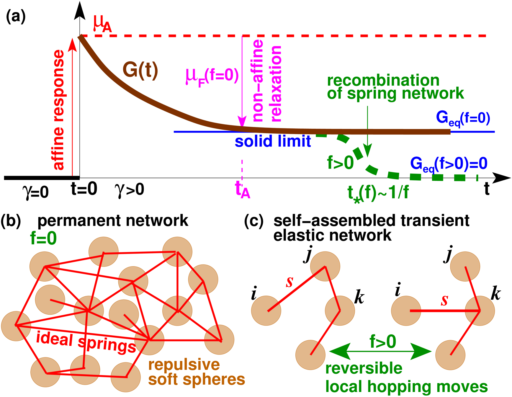
A central rheological property characterizing the linear shear-stress response in isotropic amorphous solids and glasses Alexander (1998); Hansen and McDonald (2006); Götze (2009) and visco-elastic fluids de Gennes (1979); Doi and Edwards (1986); Witten and Pincus (2004); Rubinstein and Colby (2003) is the shear relaxation modulus $G(t)$ sketched in panel (a) of Fig. 1. Experimentally, $G(t)=\delta\tau(t)/\delta\gamma$ may be obtained from the average stress increment $\delta\tau(t)$ as a function of time $t$ after a small step strain $\delta\gamma$ has been imposed at $t=0$. As indicated by the solid horizontal line in panel (a), $G(t)$ yields the equilibrium shear modulus $G_{\mathrm{eq}}$ of the system in the long-time limit for $t\gg t_{\star}$ with $t_{\star}$ being the terminal stress relaxation time Rubinstein and Colby (2003); Doi and Edwards (1986). Focusing on permanent elastic networks above the percolation threshold de Gennes (1979); Stauffer and Aharnony (1994); Ulrich et al. (2006) with a finite shear modulus $G_{\mathrm{eq}}$, as sketched in panel (b) of Fig. 1, it has been shown Wittmer et al. (2016) that $G(t)$ may be determined conveniently in computer simulations using the “simple average” expression

$$G(t)=\mu_{\mathrm{A}}-h(t)$$ (1)

with $\mu_{\mathrm{A}}=G(0)$ being the “affine shear elasticity” characterizing the canonical-affine shear transformation (Appendix A) of the system at $t=0$ Wittmer et al. (2013); Wittmer et al. (2015a, b, c); Wittmer et al. (2016) and $h(t)=\beta V/2\ \langle(\hat{\tau}(t)-\hat{\tau}(0))^{2}\rangle$ the (rescaled) mean-square displacement (MSD) of the instantaneous shear stress $\hat{\tau}(t)$. Here $\beta=1/T$ stands for the inverse temperature and $V$ for the volume of the simulation box. See Appendix B for the related definitions of the instantaneous shear stress $\hat{\tau}$ and the instantaneous affine shear elasticity $\hat{\mu}_{\mathrm{A}}$. Interestingly, the expectation value of Eq. (1) does not depend on the sampling time $\Delta t$ even if much smaller times than the terminal time $t_{\star}$ are probed Wittmer et al. (2016). For sufficiently large systems Eq. (1) can be demonstrated using the simple-average transformation behavior Allen and Tildesley (1994); Lebowitz et al. (1967) of $\mu_{\mathrm{A}}$ and $h(t)$ between the $\text{NV}\gamma\text{T}$-ensemble at constant particle number $N$, volume $V$, shear strain $\gamma$ and temperature $T$ and the conjugated $\text{NV}\tau\text{T}$-ensemble at an imposed average shear stress $\tau$ Wittmer et al. (2016).

Albeit the equilibrium shear modulus $G_{\mathrm{eq}}$ may in principal be determined from the long-time limit of Eq. (1), most numerical studies Barrat et al. (1988); Wittmer et al. (2002); Tanguy et al. (2002); Flenner and Szamel (2015); Xu et al. (2012); Wittmer et al. (2013); Wittmer et al. (2015a, b, c); Wittmer et al. (2016) use instead the stress-fluctuation formula $G_{\mathrm{eq}}=G_{\mathrm{F}}$ with

$$G_{\mathrm{F}} \equiv \mu_{\mathrm{A}}-\mu_{\mathrm{F}}=(\mu_{\mathrm{A}}-\tilde{\mu}_{\mathrm{F}})+\mu_{\star}$$ (2)

$$\mbox{and }\mu_{\mathrm{F}} \equiv \beta V\langle\delta\hat{\tau}^{2}\rangle=\tilde{\mu}_{\mathrm{F}}-\mu_{\star}$$ (3)

standing for the rescaled shear-stress fluctuations. We have introduced here for later convenience the two terms $\tilde{\mu}_{\mathrm{F}}\equiv\beta V\langle\hat{\tau}^{2}\rangle$ and $\mu_{\star}\equiv\beta V\langle\hat{\tau}\rangle^{2}$. As sketched in panel (a) of Fig. 1, $\mu_{\mathrm{F}}$ corresponds to the (free) energy relaxed by non-affine displacements after an initial canonical-affine shear strain $\delta\gamma$ is imposed. Note that $G_{\mathrm{F}}$ is a special case of the general stress fluctuation relations for elastic moduli Squire et al. (1969); Barrat et al. (1988); Lutsko (1989); Mizuno et al. (2013). As stressed elsewhere Wittmer et al. (2013); Wittmer et al. (2015a); Wittmer et al. (2016), being “fluctuations” (not “simple averages”) Allen and Tildesley (1994); Wittmer et al. (2016) the expectation values of $G_{\mathrm{F}}$, $\mu_{\mathrm{F}}$ and $\mu_{\star}$ may depend strongly on the sampling time $\Delta t$ (as often marked below by indicating $\Delta t$ as additional argument) and converge very slowly to their asymptotic static limit for $\Delta t\gg t_{\star}$. This behavior is not due to aging or equilibration problems but simply caused by the finite time needed for the stress fluctuations to explore the phase space Wittmer et al. (2013). Interestingly, using Eq. (1) and assuming time translational invariance it can be shown that $G_{\mathrm{F}}(\Delta t)$ and $G(t)$ are related by

$$G_{\mathrm{F}}(\Delta t)=\frac{2}{\Delta t^{2}}\int_{0}^{\Delta t}(\Delta t-t)\ G(t)\ \text{d}t,$$ (4)

i.e. $G_{\mathrm{F}}(\Delta t)$ is a (weighted) average of $G(t)$ foo (a, b). It converges thus more slowly to $G_{\mathrm{eq}}$ but this with a better statistics. See Ref. Wittmer et al. (2015a) and Appendix F for details.

I.2 New focus: Transient self-assembled networks

We generalize here our previous work on solid bodies Wittmer et al. (2015a); Wittmer et al. (2016) to visco-elastic liquids de Gennes (1979); Witten and Pincus (2004); Rubinstein and Colby (2003). The first goal of the present work is to introduce and to characterize numerically a simple model for transient self-assembled networks Zilman et al. (2003); Hed and Safran (2006); Testard et al. (2008); Montarnal et al. (2011); Smallenburg et al. (2013); Roldán-Vargas et al. (2013); Tonhauser et al. (2010). As sketched in panel (c) of Fig. 1, repulsive “harmonic spheres” Berthier et al. (2010, 2011) are reversibly bridged by ideal springs. It is assumed that the springs break and recombine locally with a Monte Carlo (MC) hopping frequency $f$ in a similar manner as in earlier work on equilibrium polymer systems Wittmer et al. (1998); Huang et al. (2006). As sketched by the bold dashed line in panel (a) of Fig. 1, these transient networks are shown to be simple Maxwell fluids Rubinstein and Colby (2003), i.e. the shear-stress relaxation modulus decays exponentially

$$G(t)\approx G_{\star}\exp(-x)\mbox{ with }x\equiv t/t_{\star}(f)\mbox{ for }t/t_{\mathrm{A}}\gg 1$$ (5)

with $t_{\mathrm{A}}$ being a local time scale characterizing the decay of the initial affine displacements, $t_{\star}(f)\sim 1/f$ the Maxwell time and $G_{\star}$ the intermediate plateau modulus set by the equilibrium shear modulus $G_{\mathrm{eq}}$ for permanent springs ($f=0)$. From the rheological point of view our model is very similar to patchy colloids Smallenburg et al. (2013); Roldán-Vargas et al. (2013) or “vitrimers” Montarnal et al. (2011), i.e. covalent polymer networks that can rearrange their topology via a bond shuffling mechanism. Rheologically similar self-assembled transient networks may also be formed by hyperbranched polymer chains with sticky end-groups Tonhauser et al. (2010) or microemulsions bridged by telechelic polymers Zilman et al. (2003); Hed and Safran (2006); Testard et al. (2008). While mainly keeping the sampling time $\Delta t$ constant, we systematically scan the dimensionless attempt frequency $\Delta x\equiv\Delta t/t_{\star}(f)\sim f$ from the liquid state ($\Delta x\gg 1$), where the network topology is annealed, down to the solid limit ($\Delta x\ll 1$), where the recombination events become irrelevant and the particle permutation symmetry is lifted Witten and Pincus (2004). Due to detailed balance this is done while keeping unchanged all static properties related to pair correlations. The $\Delta x$-dependence reported below for $G(t)$ or $G_{\mathrm{F}}$ thus cannot be traced back to pair correlations as often assumed for glass-forming systems Hansen and McDonald (2006); Götze (2009). By integration of the general relation Eq. (4) for a Maxwell fluid, Eq. (5), one expects in fact the shear-stress fluctuations to be given by

$$G_{\mathrm{F}}(\Delta x)\equiv\mu_{\mathrm{A}}-\mu_{\mathrm{F}}(\Delta x)=G_{\star}\ f_{\mathrm{Debye}}(\Delta x)$$ (6)

with $f_{\mathrm{Debye}}(x)=2(\exp(-x)-1+x)/x^{2}$ being the Debye function well-known in polymer physics Doi and Edwards (1986); Rubinstein and Colby (2003). We shall see that this important relation allows to interpolate our numerical data between the solid limit, where $G_{\mathrm{F}}(\Delta x)\to G_{\star}$ and $\mu_{\mathrm{F}}(\Delta x)\to\mu_{\mathrm{A}}-G_{\star}$ for $\Delta x\ll 1$, and the liquid limit, where $G_{\mathrm{F}}(\Delta x)\to 0$ and $\mu_{\mathrm{F}}(\Delta x)\to\mu_{\mathrm{A}}$ for $\Delta x\gg 1$.

Using our simple model the second goal of this study is to show that Eq. (1) does not only hold for elastic solids ($\Delta x\ll 1$) but more generally for visco-elastic bodies, i.e. for all values of $\Delta x$. We shall compare this relation to the widely assumed expression Allen and Tildesley (1994); Hansen and McDonald (2006); Duering et al. (1991); Klix et al. (2012); Flenner and Szamel (2015); Smallenburg et al. (2013)

$$G(t)=\tilde{c}(t)\mbox{ with }\tilde{c}(t)\equiv\beta V\left<\hat{\tau}(t)\hat{\tau}(0)\right>$$ (7)

being the (rescaled) shear-stress autocorrelation function (ACF). Albeit Eq. (7) is incorrect for general elastic bodies Wittmer et al. (2015a, b, c); Wittmer et al. (2016), it may be justified under the condition

$$\mu_{\mathrm{A}}\stackrel{{\scriptstyle!}}{{=}}\tilde{c}(t=0)\equiv\tilde{\mu}_{\mathrm{F}}.$$ (8)

While this condition indeed holds on average for self-assembled networks, it requires on the numerical side that either $\Delta x\gg 1$, or, equivalently, an ensemble-average over a large number $m$ of independent configurations. Being thus both in principle acceptable means to determine $G(t)$ for any $\Delta x$, this does, of course, not imply that Eq. (1) and Eq. (7) have the same statistics. We shall thus attempt to characterize the standard deviations of both relations and estimate lower bounds for the number of configurations required.

I.3 Outline

Our numerical model is formulated in Sec. II where we also address several technical questions. Our central numerical findings are then discussed in Sec. III. Carefully stating the subsequent time and ensemble averages performed, we present in Sec. III.1 the pertinent static and quasi-static properties. The MSD $h(t)$ is described in Sec. III.2 where we test Eq. (1) numerically by comparing it to the shear response modulus $G(t)$ obtained by applying explicitly a small step strain $\delta\gamma$. For the available $m=100$ configurations Eq. (7) is shown in Sec. III.3 to be a poor approximation of $G(t)$ for $\Delta x\ll 1$. The number of configurations required by, respectively, Eq. (1) and Eq. (7) are estimated in Sec. III.4. Section IV contains a summary of the present work and an outline of open questions. Less central issues are regrouped in the Appendix. Concepts and definitions already stated elsewhere Wittmer et al. (2013); Wittmer et al. (2015a, b, c); Wittmer et al. (2016) are reminded in Appendix A and Appendix B. The theoretical derivations of Eq. (2) and Eq. (1) can be found in Appendix C and Appendix D. Being not based on the transformation behavior between conjugated ensembles used in our previous work Wittmer et al. (2015b, c); Wittmer et al. (2016)), these direct demonstrations are relevant for (complex) liquid systems with vanishing equilibrium shear modulus the present study focuses on. Computational results related to the sampling time $\Delta t$ are briefly discussed in Appendix E and Appendix F.

Figure 2: (Color online) Some technical details: (a) Model Hamiltonian with the bold line indicating the purely repulsive interaction between “harmonics spheres” Berthier et al. (2010) and the thin line the ideal spring between connected beads, (b) distribution $p(r)$ of spring lengths $r$ showing a maximum around the minimum of the spring potential at $\mbox{$R_{\rm sp}$}=2$ and (c) distribution $p(\mbox{$n_{\rm sp}$})$ of the number of springs $n_{\rm sp}$ being connected to a bead showing a maximum at $\mbox{$n_{\rm sp}$}\approx 8$. Only a negligible number of beads is not connected ($\mbox{$n_{\rm sp}$}=0$) or are dangling ends ($\mbox{$n_{\rm sp}$}=1$). In the current work $\mbox{$n_{\rm sp}$}\leq 12$ is imposed. The distributions shown in panel (b) and (c) are identical for all attempt frequencies $f$ due to detailed balance.

Figure 3: (Color online) Snapshot of small square subvolume of linear length $10$ containing $103$ beads (disks) connected by $407$ springs (straight lines). The width of the spring lines is proportional to the energy of the spring potential, Eq. (10). Short springs with $r<\mbox{$R_{\rm sp}$}=2$ repel the beads (green lines), longer springs (red lines) keep them together.

II Algorithm and technical details

As sketched in Fig. 1 we use a generic model for self-assembled elastic networks in $d=2$ dimensions where beads are reversibly bridged by ideal springs. These springs recombine locally with a Monte Carlo (MC) attempt frequency $f$. Lennard-Jones (LJ) units are used throughout this work Allen and Tildesley (1994) and the particle mass $m$, Boltzmann’s constant $k_{\rm B}$ and the temperature $T=1/\beta$ are set to unity. Periodic simulation boxes of constant volume $V=L^{d}$ and linear box size $L=100$ are used. A standard Euclidean metric with a shear strain $\gamma=0$ can be assumed (square box) if not stated otherwise. Moreover, the total number $N_{\rm b}$ of beads and the number $N_{\rm sp}$ of springs are kept constant in the present work.

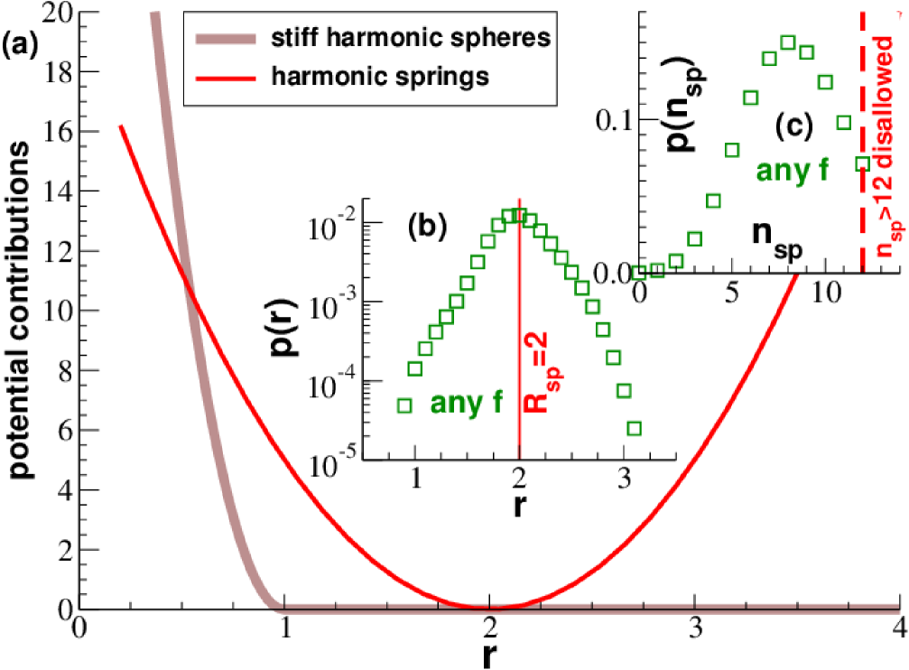
As shown by the bold solid line in panel (a) of Fig. 2, the particles are modeled as “harmonic spheres” Berthier et al. (2010) interacting through the purely repulsive potential

$$\mbox{$U_{\rm b}$}(r)=\frac{\mbox{$K_{\rm b}$}}{2}\left(r-\mbox{$R_{\rm b}$}\right)^{2}\mbox{ for }r\leq\mbox{$R_{\rm b}$}$$ (9)

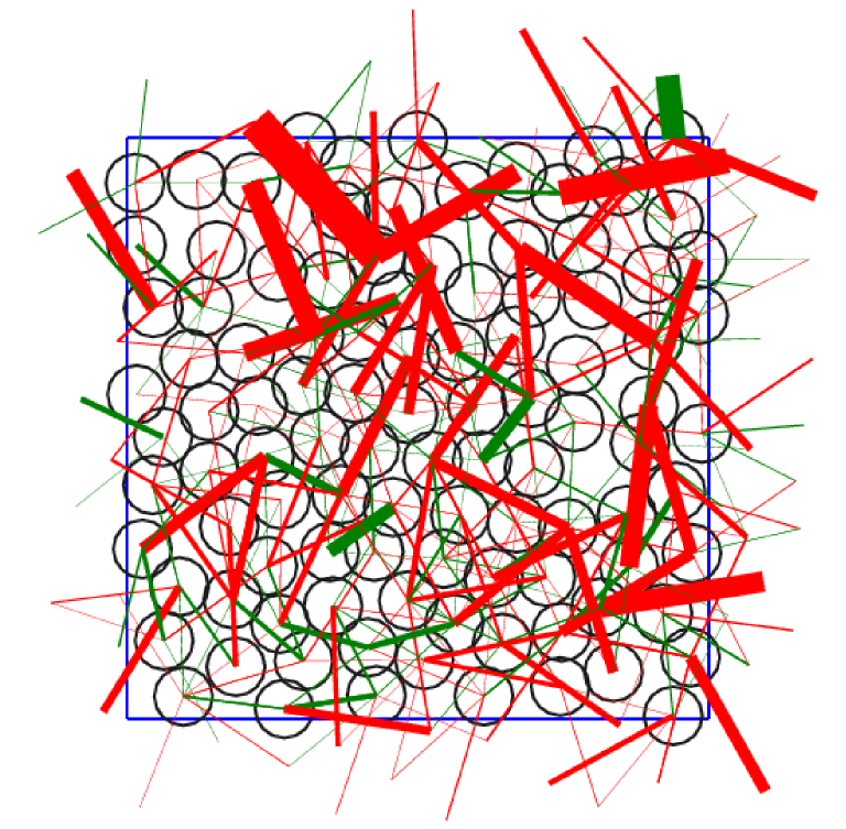
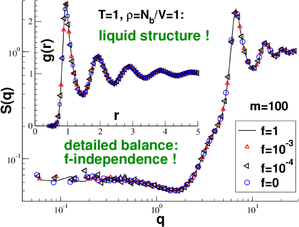
and $\mbox{$U_{\rm b}$}(r)=0$ elsewhere. The minimum of the shifted harmonic potential is used as cut-off to avoid truncation effects and impulsive corrections for the determination of the affine shear elasticity $\mu_{\mathrm{A}}$ as described in Ref. Xu et al. (2012). The bead diameter is arbitrarily set to unity, $\mbox{$R_{\rm b}$}=1$, and a rather stiff spring constant $\mbox{$K_{\rm b}$}=100$ is used making the beads very repulsive. The simulation box contains $\mbox{$N_{\rm b}$}=10^{4}$ beads, i.e. the number density $\rho=\mbox{$N_{\rm b}$}/V$ of the beads is set to unity. Due to the strong repulsion and the high number density, the bead distribution is always macroscopically homogeneous and the overall density fluctuations are weak. This has been checked using snapshots, as the one shown in Fig. 3, and the standard radial pair correlation function $g(r)$ and its Fourier transform $S(q)$ Allen and Tildesley (1994) as presented in Fig. 4.

The bonding of two beads is described by

$$\mbox{$U_{\rm sp}$}(r)=\frac{\mbox{$K_{\rm sp}$}}{2}\left(r-\mbox{$R_{\rm sp}$}\right)^{2}$$ (10)

with $\mbox{$R_{\rm sp}$}=2$ and $\mbox{$K_{\rm sp}$}=10$ as shown by the thin line in panel (a) of Fig. 2. Note that the minimum $R_{\rm sp}$ of the bonding potential is much larger than the bead diameter $R_{\rm b}$. There is thus no repulsion between two beads at $r\approx\mbox{$R_{\rm sp}$}$ and no sudden acceleration is felt (on average) if a bond is broken. As seen in panel (b) of Fig. 2, the probability distribution $p(r)$ of springs of length $r$ has a sharp maximum at $R_{\rm sp}$ and the number of springs with $r<1$ or $r>3$ is negligible. Our box contains a constant number $\mbox{$N_{\rm sp}$}=4\mbox{$N_{\rm b}$}$ of springs, i.e. on average a bead is connected by $\mbox{$n_{\rm sp}$}=8$ springs. This corresponds roughly to the maximum of the distribution $p(\mbox{$n_{\rm sp}$})$ of the number $n_{\rm sp}$ of springs connected to a given bead presented in panel (c) of Fig. 2. Since there is no direct interaction (repulsion) between the springs, the maximum number of springs connected to a bead is limited to $\mbox{$n_{\rm sp}$}=12$ foo (c).

Figure 4: (Color online) Pair correlations for several attempt frequencies $f$. Inset: Radial pair correlation distribution function $g(r)$ with $r$ being the distance between two beads Hansen and McDonald (2006). Main panel: Total coherent structure function $S(q)$ with $q$ being the length of the wavevector.

As sketched in panel (c) of Fig. 1, the network is reorganized by attempting with a frequency $f$ local hopping moves for each spring. This is done by choosing first randomly a spring $s$ connecting two beads $i$ and $j$. If the spring length $r$ is smaller than a cut-off radius $\mbox{$r_{\rm c}$}=5$, the connection to one bead is broken, say bead $j$, and we attempt to reconnect the spring to a randomly chosen monomer $k$ (different from $i$ or $j$) taken randomly from a neighbor list of beads with distance $r<\mbox{$r_{\rm c}$}$ from the pivot monomer $i$ and having less than $\mbox{$n_{\rm sp}$}=12$ springs attached foo (d). Using the energy change due to the different lengths of the suggested and the original spring state, the move is accepted subjected to a standard Metropolis acceptance criterion Allen and Tildesley (1994); Landau and Binder (2000). The parameter $r_{\rm c}$ is chosen sufficiently small to reduce the neighbor list and to yield a reasonable, not too small acceptance rate $A\approx 0.1$ (found to be identical for all $f$). The computational load required by the reorganization of the network topology becomes negligible below an attempt frequency $f=0.01$.

$f$	$\Delta x$	$e$	$P$	$\mu_{\mathrm{A}}$	$\tilde{\mu}_{\mathrm{F}}$	$\mu_{\star}$	$G_{\mathrm{F}}$
1.0	6250	2.442	1.73	33.1	$33$	$\approx 0$	$\approx 0$
0.1	625	2.442	1.73	33.1	$33(0.1)$	$\approx 0$	$\approx 0$
0.01	62.5	2.442	1.72	33.1	$33(0.3)$	$0.5(0.1)$	$0.5(0.3)$
E-03	6.25	2.443	1.73	33.1	$36(1.1)$	$5(0.7)$	$2.9(0.8)$
E-04	0.625	2.442	1.73	33.2	$32(1.9)$	$13(1.9)$	$13.6(0.4)$
E-05	0.0625	2.441	1.74	33.2	$29(1.8)$	$14(1.8)$	$17.4(0.1)$
E-06	6.25E-03	2.443	1.73	33.3	$35(2.7)$	$20(2.7)$	$17.8$
E-07	6.25E-04	2.442	1.73	33.2	$32(2.5)$	$18(2.5)$	$17.9$
0	0	2.440	1.74	33.1	$32(2.3)$	$17(2.3)$	$17.9$

Table 1: Some properties as a function of the attempt frequency $f$: $\Delta x\equiv\Delta t/t_{\star}(f)$ with $\Delta t=10^{5}$ and $t_{\star}(f)=16/f$, excess energy per bead $e$, average normal pressure $P$, affine shear elasticity $\mu_{\mathrm{A}}$, contributions $\tilde{\mu}_{\mathrm{F}}$ and $\mu_{\star}$ to the shear-stress fluctuation $\mu_{\mathrm{F}}=\tilde{\mu}_{\mathrm{F}}-\mu_{\star}$ and $G_{\mathrm{F}}=\mu_{\mathrm{A}}-\mu_{\mathrm{F}}$. All data are averaged over $m=100$ configurations. Error bars (for values $>0.1$) are indicated for the last three columns.

In addition to the MC moves changing the connectivity matrix of the network standard velocity-Verlet molecular dynamics (MD) Allen and Tildesley (1994) is used to move the beads through the phase space. The temperature $T=1$ is imposed using a Langevin thermostat of friction constant $\zeta=1$. This allows to suppress long-range hydrodynamic modes otherwise relevant for two-dimensional systems. A velocity-Verlet time step $\delta t_{\mathrm{MD}}=10^{-2}$ is used. Every time step $\delta t_{\mathrm{MD}}$ a certain number of springs corresponding to the frequency $f$ is considered for an MC hopping move. We start by equilibrating $m=100$ independent configurations at $f=1$. The frequency is then decreased with steps $f=1,0.3,0.1,0.03,0.01,\ldots,10^{-7}$ and finally $f=0$. At each step the configurations are tempered over a time interval $t_{\mathrm{temp}}=10^{4}$ and then sampled over $t_{\mathrm{traj}}=10^{5}$. Due to detailed balance changing $f$ does not change the standard static properties, such as described by the pair correlation functions $g(r)$ and $S(q)$ (Fig. 4) or the energy per bead $e$ or the normal pressure $P$ shown in Table 1. As we have checked, one could have also considered a much more rapid quench without changing these static properties. As seen from Fig. 3, we obtain homogeneous and isotropic elastic networks well above the percolation threshold de Gennes (1979); Stauffer and Aharnony (1994). This is consistent with the large values $G_{\mathrm{F}}\approx 18$ for small $f$ in Table 1.

III Computational results

III.1 Static and quasi-static properties

Figure 5: Various “static” and “quasi-static” properties vs. $\Delta x(f)\equiv\Delta t/t_{\star}(f)$ with $\Delta t=10^{5}$ and $t_{\star}(f)=16/f$. The data indicated for the smallest $\Delta x$ correspond to $f=0$. The prediction Eq. (6) is indicated by the solid and the dash-dotted lines. Note that $\tilde{\mu}_{\mathrm{F}}\approx\mu_{\mathrm{A}}$ and $\mu_{\star}\approx G_{\mathrm{F}}$ for all $\Delta x$.

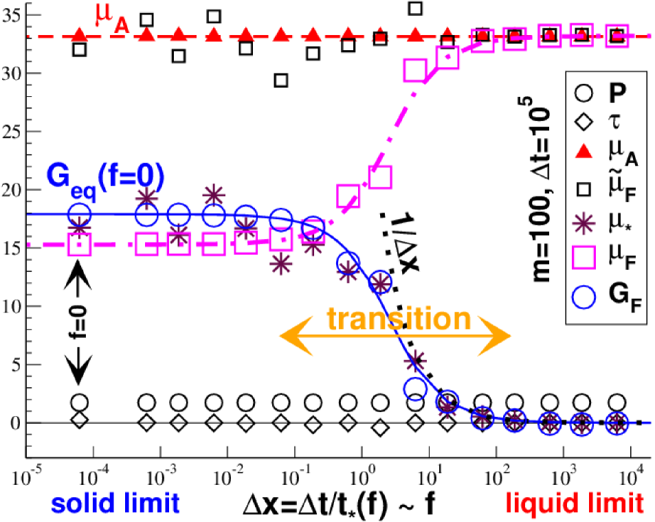
We begin the description of our transient networks by discussing the static and quasi-static properties presented in Fig. 5. For every attempt frequency $f$ we sample $m=100$ configurations over a fixed sampling time $\Delta t=t_{\mathrm{traj}}=10^{5}$. For each trajectory we store every $\delta t_{\mathrm{MD}}=0.01$ instantaneous properties such as the normal pressure $\hat{P}$, the shear stress $\hat{\tau}$ or the affine shear elasticity $\hat{\mu}_{\mathrm{A}}$ as defined in Appendix B. Using these instantaneous values $\hat{a}$ we then sample the time averages $\overline{\hat{a}}$ and $\overline{\hat{a}^{2}}$ over the $\Delta t/\delta t_{\mathrm{MD}}$ entries for each configuration. Using these time averages we obtain for each configuration an observable $\hat{o}$ and compute its first moment ${o}=\langle\hat{o}\rangle$ over the $m$ configurations. (The second moment $\langle\hat{o}^{2}\rangle$ will be considered in Sec. III.4.) The following properties

$$\hat{o}=\overline{\hat{P}} \Rightarrow {o}=P$$ (11)

$$\hat{o}=\overline{\hat{\tau}} \Rightarrow {o}=\tau$$ (12)

$$\hat{o}=\overline{\hat{\mu}_{\mathrm{A}}} \Rightarrow {o}=\mu_{\mathrm{A}}$$ (13)

$$\hat{o}=\beta V\overline{\hat{\tau}^{2}} \Rightarrow {o}=\tilde{\mu}_{\mathrm{F}}$$ (14)

$$\hat{o}=\beta V\overline{\hat{\tau}}^{2} \Rightarrow {o}=\mu_{\star}$$ (15)

$$\hat{o}=\beta V(\overline{\hat{\tau}^{2}}-\overline{\hat{\tau}}^{2}) \Rightarrow {o}=\mu_{\mathrm{F}}=\tilde{\mu}_{\mathrm{F}}-\mu_{\star}$$ (16)

$$\hat{o}=\overline{\hat{\mu}_{\mathrm{A}}}-\beta V(\overline{\hat{\tau}^{2}}-\overline{\hat{\tau}}^{2}) \Rightarrow {o}=G_{\mathrm{F}}=\mu_{\mathrm{A}}-\mu_{\mathrm{F}}$$ (17)

are presented in Fig. 5 using log-linear coordinates. The vertical axis has the dimension energy per volume. The horizontal axis has been made dimensionless using $\Delta x\equiv\Delta t/t_{\star}(f)$ with $t_{\star}(f)=16/f$ as shown below in Sec. III.2. (See Appendix E for the scaling with sampling time $\Delta t$ at fixed $f$.) In the “solid limit” ($\Delta x\ll 1$) only few spring recombinations can occur and the networks thus behave as solid bodies, while in the “liquid limit” ($\Delta x\gg 1$) the particles may freely change their neighbors.

As may be seen from Table 1 or Fig. 5, the pressure $P$, the shear stress $\tau$, the affine shear elasticity $\mu_{\mathrm{A}}$ and the contribution $\tilde{\mu}_{\mathrm{F}}$ to the shear-stress fluctuation $\mu_{\mathrm{F}}$ do not depend on $\Delta x$, i.e. the same values $P\approx 1.7$, $\tau\approx 0$ and $\mu_{\mathrm{A}}\approx\tilde{\mu}_{\mathrm{F}}\approx 33.2$ have been obtained for all $f$. The expectation values of these truly “static” properties cannot depend on $\Delta t$ or on $f$ since time and ensemble averages do “commute” Wittmer et al. (2016), i.e. can be exchanged as

$$\left<\overline{\hat{a}}\right>=\overline{\left<\hat{a}\right>}\mbox{ with }\hat{a}=\hat{P},\hat{\tau},\hat{\mu}_{\mathrm{A}}\mbox{ or }\beta V\hat{\tau}^{2},$$ (18)

and since the thermodynamic ensemble average $\langle\ldots\rangle$ does not depend on $\Delta t$ or $f$. Although $P$, $\tau$, $\mu_{\mathrm{A}}$ and $\tilde{\mu}_{\mathrm{F}}$ are all $\Delta x$-independent, this does not imply that they have the same statistics. The “simple averages” $P$, $\tau$ and $\mu_{\mathrm{A}}$ have been obtained with a high precision while the “fluctuation” $\tilde{\mu}_{\mathrm{F}}$ is rather noisy Allen and Tildesley (1994); Wittmer et al. (2016).

A qualitatively different behavior is observed for the observables $\mu_{\star}(\Delta x)$, $\mu_{\mathrm{F}}(\Delta x)$ and $G_{\mathrm{F}}(\Delta x)$ also represented in Fig. 5. Please note that Eq. (18) does not hold for these properties as may be seen for $\mu_{\star}(\Delta x)=\langle\overline{s}^{2}\rangle\geq 0$ with $s=\sqrt{\beta V}\hat{\tau}$. Obviously, this differs from $\overline{\langle s\rangle^{2}}\sim\tau^{2}$ which vanishes due to symmetry for all $\Delta x$ for a sufficiently large ensemble. Ergodicity implies $\overline{s}\to\langle s\rangle$ for large $\Delta x$ and all $\Delta x$-effects become thus irrelevant. As seen from Fig. 5, this implies $\mu_{\star}(\Delta x)\to\beta V\tau^{2}=0$ for $\Delta x\gg 1$. Similarly, one observes $G_{\mathrm{F}}(\Delta x)=\mu_{\mathrm{A}}-\mu_{\mathrm{F}}(\Delta x)\to 0$ and thus $\mu_{\mathrm{F}}(\Delta x)\to\mu_{\mathrm{A}}$ as expected for liquids Wittmer et al. (2013); Wittmer et al. (2015a). The quasi-static properties become also constant for $\Delta x\ll 1$ where $G_{\mathrm{F}}(\Delta x)\to G_{\mathrm{eq}}(f=0)\approx 18$ and $\mu_{\mathrm{F}}(\Delta x)\to\mu_{\mathrm{F}}(f=0)\approx 15.$ Interestingly, the transition between both limits around $\Delta x\approx 1$ is rather broad corresponding to several orders of magnitude. Our data are nicely fitted over the full range of $\Delta x$ by the expected behavior Eq. (6) for a Maxwell fluid as indicated by the thin solid line for $G_{\mathrm{F}}(\Delta x)\approx\mu_{\star}(\Delta x)$ and by the dash-dotted line for $\mu_{\mathrm{F}}(\Delta x)=\mu_{\mathrm{A}}-G_{\mathrm{F}}(\Delta x)$. We remind that $f_{\mathrm{Debye}}(x)\to 1$ for $x\to 0$ and $f_{\mathrm{Debye}}(x)\to 2/x$ for $x\gg 1$. This implies that $G_{\mathrm{F}}(\Delta x)$ decays as $2G_{\star}/\Delta x$ in the liquid limit as shown by the dotted line.

Let us finally consider the scaling of the two contributions $\tilde{\mu}_{\mathrm{F}}$ and $\mu_{\star}(\Delta x)$ to the shear-stress fluctuation $\mu_{\mathrm{F}}(\Delta x)$. As seen from Fig. 5, we have $\tilde{\mu}_{\mathrm{F}}\approx\mu_{\mathrm{A}}$ in agreement with Eq. (8) and in addition

$$\mu_{\star}(\Delta x)\approx G_{\mathrm{F}}(\Delta x)$$ (19)

for all $\Delta x$. As already stressed, the expectation value of $\tilde{\mu}_{\mathrm{F}}(\Delta x)$ does not depend on $\Delta x$. This must especially hold for large $\Delta x$ where the average shear stress $\overline{s}\equiv\sqrt{\beta V}\ \overline{\hat{\tau}}$ must vanish for each configuration and, hence, $\mu_{\star}(\Delta x)=\langle\overline{s}^{2}\rangle\approx 0$. Since the stress-fluctuation estimate $G_{\mathrm{F}}$ for the shear modulus, Eq. (2), must also vanish in the liquid limit, this implies $0\approx\mu_{\mathrm{A}}-\tilde{\mu}_{\mathrm{F}}$ for $\Delta x\gg 1$. Since $\tilde{\mu}_{\mathrm{F}}$ does not depend on $\Delta x$, this demonstrates Eq. (8) and using Eq. (2) this implies in turn Eq. (19). Please note that Eq. (8) and Eq. (19) do not hold for an arbitrary elastic body as shown, e.g., in Ref. Wittmer et al. (2016). In fact they do not necessarily hold even for one configuration of our ensemble if $\Delta x\ll 1$. As we shall see in Sec. III.4, they only apply for $\Delta x\gg 1$ or for an average over a large number $m$ of configurations for $\Delta x\ll 1$.

Figure 6: (Color online) Shear-stress MSD $h(t)$ for different frequencies $f$. Main panel: The MSD increases as $h(t)\sim t^{2}$ for small times $t\ll t_{\mathrm{A}}$ (thin solid line), shows an intermediate plateau with $h(t)\approx\mu_{\mathrm{F}}(f=0)$ for $t_{\mathrm{A}}\ll t\ll t_{\star}(f)$ (bold solid line) and approaches $\mu_{\mathrm{A}}$ (dashed line) for even larger times $t\gg t_{\star}(f)$. Inset: Comparison of $y(x)=(\mu_{\mathrm{A}}-h(t))/G_{\star}$ with $x=t/t_{\star}(f)$, $t_{\star}(f)=16/f$ and $G_{\star}=G_{\mathrm{eq}}(f=0)$ with the shear-stress response modulus $G(t)/G_{\star}$ for $f=0.01$ and $f=10^{-6}$ obtained from the shear-stress increment $\left<\delta\hat{\tau}(t)\right>$ after applying a step-strain increment $\delta\gamma=0.01$ at $t=0$.

III.2 Shear-stress mean-square displacement

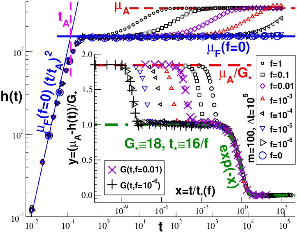
The shear-stress MSD $h(t)$ is presented in Fig. 6 for a broad range of attempt frequencies $f$. The data have been computed using

$$h(t)\equiv\frac{\beta V}{2}\left<\overline{\left(\hat{\tau}(t+t_{0})-\hat{\tau}(t_{0})\right)^{2}}\right>$$ (20)

where the horizontal bar stands for the gliding average over $t_{0}$ Allen and Tildesley (1994) for each configuration using a fixed time window $\Delta t=10^{5}$ and $\left<\ldots\right>$ for the ensemble average over $m=100$ configurations. Time and ensemble averages commute, Eq. (18), i.e. the expectation value of the MSD does not depend explicitly on the sampling time as emphasized in Ref. Wittmer et al. (2016). Let us focus first on the main panel of Fig. 6 where the unscaled $h(t)$ is presented using double-logarithmic coordinates. Three dynamical regimes can be distinguished corresponding to the time windows (i) $t\ll t_{\mathrm{A}}$, (ii) $t_{\mathrm{A}}\ll t\ll t_{\star}(f)$ and (iii) $t_{\star}(f)\ll t$. The MSD does not depend on the attempt frequency $f$ in the first two regimes, i.e. the reorganization of the spring network is still irrelevant. The two indicated solid lines form a lower envelope for $h(t)$ for $f\to 0$. The MSD increases as $h(t)\sim t^{2}$ in the first regime foo (e) and shows an intermediate plateau with $h(t)\approx\mu_{\mathrm{F}}(f=0)$ in the second. Following Refs. Wittmer et al. (2015c); Wittmer et al. (2016) the value of the crossover time $t_{\mathrm{A}}\approx 0.12$ is fixed by matching the asymptotics as indicated by the vertical dash-dotted line. The second regime is consistent with the equilibrium modulus of the quenched network $G_{\mathrm{eq}}(f=0)=G_{\mathrm{F}}(f=0)\approx\mu_{\mathrm{A}}-h(t)\approx 18$ for $t_{\mathrm{A}}\ll t\ll t_{\star}(f)$. The spring recombinations become relevant for times of order $t_{\star}(f)$. Depending on $f$ the MSD $h(t)$ increases now further approaching from below the long time limit $h(t)\to\mu_{\mathrm{F}}(f>0)=\mu_{\mathrm{A}}$ and the $f$-dependence thus drops out again.

We have yet to verify the scaling of the network relaxation time $t_{\star}(f)$ which characterizes the crossover from the second to the third regime. This is done in the inset of Fig. 6 where $h(t)$ is replotted using a half-logarithmic representation. The axes are made dimensionless by plotting $y(x)=(\mu_{\mathrm{A}}-h(t))/G_{\star}$ as a function of the reduced time $x\equiv t/t_{\star}(f)$ where we set $G_{\star}\equiv G_{\mathrm{eq}}(f=0)$ for the intermediate plateau modulus and $t_{\star}(f)\equiv 16/f$ for the network relaxation time. This rescaling leads to a perfect collapse of the data for $x\gg x_{\mathrm{A}}(f)\equiv t_{\mathrm{A}}/t_{\star}(f)$, especially for the $f$-dependent regime seen in the main panel. Moreover, the reduced MSD is seen to decay exponentially as $y(x)=\exp(-x)$ for $x\gg x_{\mathrm{A}}(f)$ (dash-dotted line). The prefactor $16$ for $t_{\star}(f)$ has been introduced for convenience. For not too small attempt frequencies $f\geq 10^{-4}$, the exponential decay and the scaling of the relaxation time $t_{\star}(f)$ may also be checked by plotting the unscaled $\mu_{\mathrm{A}}-h(t)$ vs. $t$ using a linear-logarithmic representation (not shown).

Due to the uncorrelated recombinations of the springs a Maxwell fluid relaxation is expected for our simple model. The observed exponential decay, Eq. (5), thus confirms Eq. (1). This is also demonstrated by the comparison with the directly computed relaxation moduli for the two attempt frequencies $f=0.01$ and $f=10^{-6}$ corresponding, respectively, to the liquid limit ($\Delta x=62.5\gg 1$) and the solid limit ($\Delta x=0.00625\ll 1$). As in our recent studies on permanent elastic networks Wittmer et al. (2015a, b, c); Wittmer et al. (2016) the relaxation modulus has been computed from the shear-stress increment $\left<\delta\hat{\tau}(t)\right>$ with $\delta\hat{\tau}(t)\equiv\hat{\tau}(t)-\hat{\tau}(0^{-})$ measured after a step-strain $\delta\gamma=0.01$ has been applied at $t=0$. This was done by applying a canonical-affine shear transformation (Appendix A) and by averaging over $m=100$ independent configurations. The perfect data collapse for all times confirms Eq. (1).

Figure 7: (Color online) Rescaled shear-stress ACF $\tilde{c}(t)/G_{\star}$ vs. dimensionless time $x=t/t_{\star}(f)$ for a broad range of $f$. Also indicated are the similarly rescaled relaxation moduli $G(t)$ obtained for $f=0.01$ and $f=10^{-6}$ by applying a step strain $\delta\gamma=0.01$. The scaling clearly fails for small $f$ (small $\Delta x$).

III.3 Shear-stress auto-correlation function

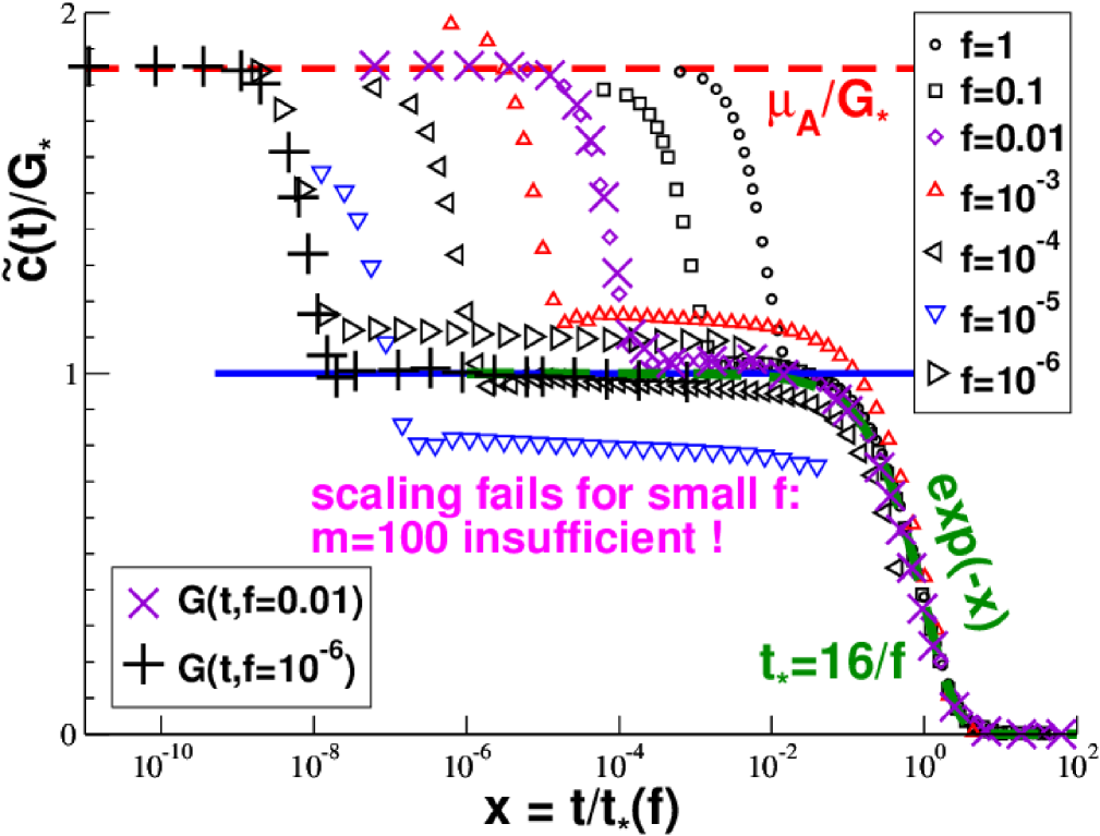
Instead of using the MSD $h(t)$ the response modulus is generally estimated in computational studies using the shear-stress ACF $\tilde{c}(t)\equiv\beta V\langle\overline{\hat{\tau}(t+t_{0})\hat{\tau}(t_{0})}\rangle$ presented in Fig. 7. Time and ensemble averages do again commute and the expectation value does thus not depend on $f$ or $\Delta t$. As suggested in Ref. Wittmer et al. (2016), one can instead of using the MSD $h(t)$ and Eq. (1) equivalently determine the relaxation modulus using

$$G(t)=\mu_{\mathrm{A}}-\tilde{\mu}_{\mathrm{F}}+\tilde{c}(t).$$ (21)

This is justified under the condition that the measured values for $\mu_{\mathrm{A}}$ and $\tilde{\mu}_{\mathrm{F}}$ for each $f$ are taken. Due to the exact identity Doi and Edwards (1986)

$$h(t)=\tilde{c}(0)-\tilde{c}(t)=\tilde{\mu}_{\mathrm{F}}-\tilde{c}(t)$$ (22)

this yields precisely the same results (not shown) as already presented in the inset of Fig. 6. Please note that for a general solid body, $\mu_{\mathrm{A}}-\tilde{\mu}_{\mathrm{F}}$ may be very different from zero and cannot be neglected in general Wittmer et al. (2016). Albeit the expectation value of this difference (obtained for asymptotically large $m$ or $\Delta x$) does vanish for any liquid (Fig. 5), the difference found for $m=100$ configurations is apparently not small enough. This explains the bad scaling for small $f$ shown in Fig. 7 where $\tilde{c}(t)/G_{\star}$ is traced as a function of $x=t/t_{\star}$ as in the inset of Fig. 6. The approximation Eq. (7) thus does not have the same status as the fundamental relation Eq. (1).

Figure 8: (Color online) Error bars $\delta o/\sqrt{m}$ for $o=\mu_{\mathrm{A}}$, $\tilde{\mu}_{\mathrm{F}}$ and $G_{\mathrm{F}}=\mu_{\mathrm{A}}-\mu_{\mathrm{F}}$ as a function of $\Delta x=\Delta t/t_{\star}(f)$. The error bars for $\mu_{\mathrm{A}}$ are several orders of magnitude smaller than those for $\tilde{\mu}_{\mathrm{F}}$. The deviations from $\mu_{\mathrm{A}}-\tilde{\mu}_{\mathrm{F}}=0$ observed in Fig. 7 for small $f$ are thus due to the fluctuations of $\tilde{\mu}_{\mathrm{F}}$.

III.4 Minimal number of configurations required

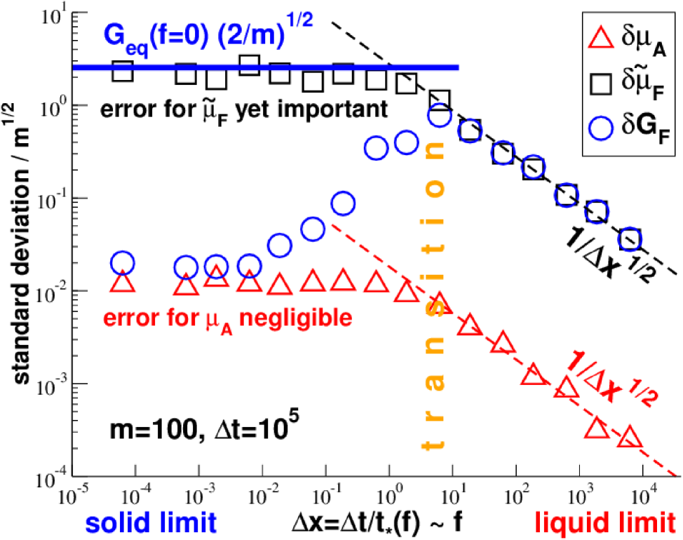
Using the $m$ independent configurations for each $f$ we have computed the standard deviations $\delta{o}\equiv(\langle\hat{o}^{2}\rangle-\langle\hat{o}\rangle^{2})^{1/2}$ and error bars $\delta{o}/\sqrt{m}$ associated with the average properties $\langle\hat{o}\rangle$ discussed above. Let us first summarize the standard deviations $\delta\mu_{\mathrm{A}}$, $\delta\tilde{\mu}_{\mathrm{F}}$ and $\delta G_{\mathrm{F}}$ associated to $\mu_{\mathrm{A}}$, $\tilde{\mu}_{\mathrm{F}}$ and $G_{\mathrm{F}}=\mu_{\mathrm{A}}-\mu_{\mathrm{F}}$. The corresponding error bars are traced in Fig. 8. As one expects assuming an increasing number $\propto\Delta x$ of independent networks probed by each configuration, all properties decay as $1/\sqrt{\Delta x}$ (dashed lines) in the liquid limit ($\Delta x\gg 1$). Note that $\delta\mu_{\mathrm{A}}$ and $\delta\tilde{\mu}_{\mathrm{F}}$ become constant for $\Delta x\ll 1$ where each configuration only probes one network topology. As indicated by the bold horizontal line foo (f),

$$\delta\tilde{\mu}_{\mathrm{F}}\approx\sqrt{2}G_{\mathrm{eq}}(f=0)\mbox{ for }\Delta x\ll 1.$$ (23)

Interestingly, $\delta G_{\mathrm{F}}$ reveals a qualitatively different non-monotonous behavior with a clear maximum at the transition at $\Delta x\approx 1$ between the liquid and the solid limit. While $\delta G_{\mathrm{F}}\approx\delta\tilde{\mu}_{\mathrm{F}}$ for $\Delta x\gg 1$, $\delta G_{\mathrm{F}}$ becomes several orders of magnitude smaller than $\delta\tilde{\mu}_{\mathrm{F}}$ for $\Delta x\ll 1$ and even becomes similar to $\delta\mu_{\mathrm{A}}$ for very small $\Delta x$. More details on the fluctuations of static properties (especially on their scaling with system size) will be given elsewhere.

Figure 9: (Color online) Standard deviations $\delta(\mu_{\mathrm{A}}-h(t))$ (filled symbols) and $\delta\tilde{c}(t)$ (open symbols) for several attempt frequencies $f$ as indicated. While $\delta\tilde{c}(t)$ becomes similar to this bound for $\Delta x\ll 1$, $\delta(\mu_{\mathrm{A}}-h(t))$ is orders of magnitude smaller in the same limit. The thin horizontal lines indicate $\delta G_{\mathrm{F}}(f)$ for $f=0$ (bottom), $f=10^{-5}$, $f=0.01$ and $10^{-3}$ (top). $\delta(\mu_{\mathrm{A}}-h(t))$ is seen to approach this limit for $t\to\Delta t$.

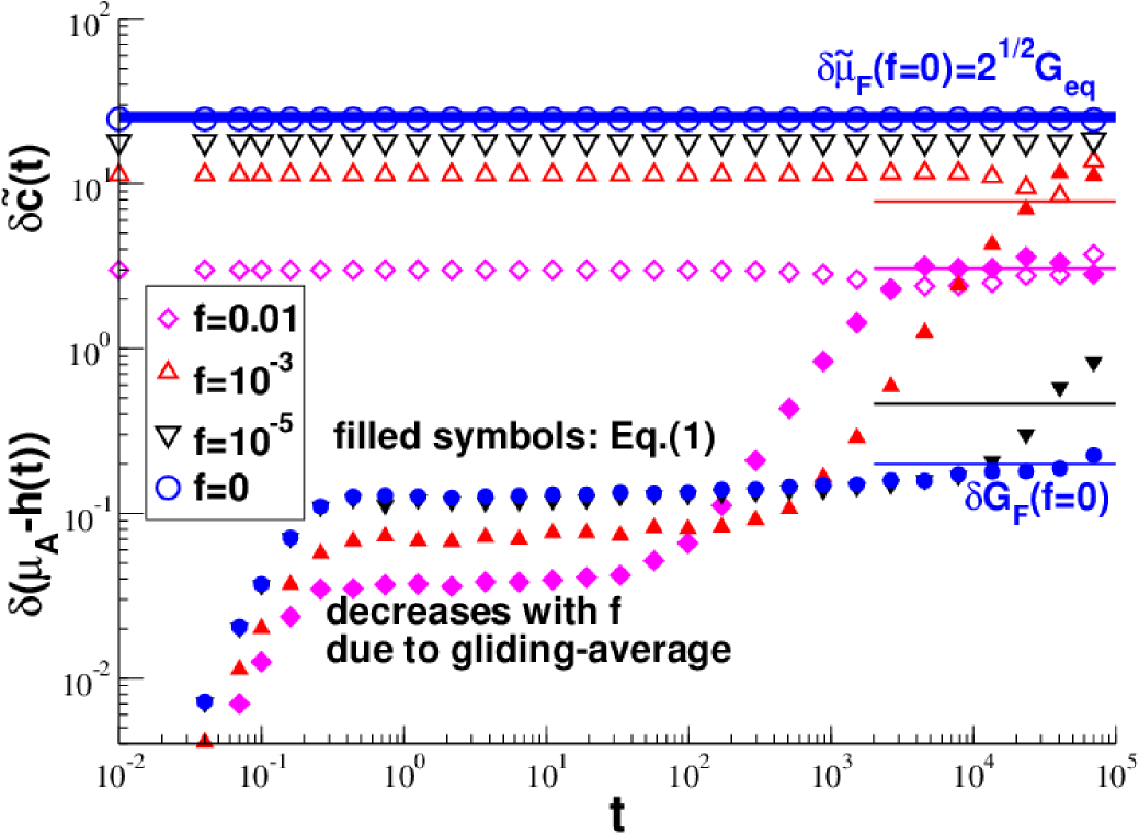
Figure 9 presents the standard deviations $\delta(\mu_{\mathrm{A}}-h(t))$ and $\delta\tilde{c}(t)$ associated with Eq. (1) and Eq. (7). $\delta\tilde{c}(t)$ is apparently time-independent. One verifies that

$$\delta\tilde{c}(t)\approx\delta(\mu_{\mathrm{A}}-\tilde{\mu}_{\mathrm{F}})\approx\delta\tilde{\mu}_{\mathrm{F}},$$ (24)

i.e. the noise is set by the fluctuations of the neglected term $\mu_{\mathrm{A}}-\tilde{\mu}_{\mathrm{F}}$. (As known from Fig. 8, $\delta\mu_{\mathrm{A}}$ is negligible.) The limit Eq. (23) for $\delta\tilde{\mu}_{\mathrm{F}}$ is thus also an upper bound for $\delta\tilde{c}(t)$ (bold horizontal line). The time-dependence of $\delta(\mu_{\mathrm{A}}-h(t))$ is more intricate (filled symbols). One (slightly trivial) reason for this is that gliding averages are used, Eq. (20), which reduce more efficiently the fluctuations for short times and higher frequencies (where more statistically independent networks are probed). We thus observe that $\delta(\mu_{\mathrm{A}}-h(t))\approx\delta h(t)$ increases monotonously with time. It becomes similar to $\delta G_{\mathrm{F}}(f)$ for $t\to\Delta t$ as indicated by thin horizontal lines. We emphasize that $\delta(\mu_{\mathrm{A}}-h(t))$ is several orders of magnitude smaller than $\delta\tilde{c}(t)$ for most times $t$ and attempt frequencies $f$. Both fluctuations become similar only for large times $t\approx\Delta t$ in the liquid limit above $\Delta x\approx 1$.

The goal is now to characterize roughly the lower bound $m_{\mathrm{min}}$ of configurations required for a given $\Delta x$ for both methods Eq. (1) and Eq. (7). Let us suppose that the relaxation modulus $G(t)$ is needed with a fixed precision $\delta G$, say $\delta G=1$. As explained above, the problem with Eq. (7) is that $\tilde{\mu}_{\mathrm{F}}$ is a strongly fluctuating quantity. Using Eq. (24) this leads to the criterion

$$m\gg m_{\mathrm{min}}=(\delta\tilde{\mu}_{\mathrm{F}}/\delta G)^{2}\ \mbox{ for Eq.~{}(\ref{eq_keyapprox}).}$$ (25)

According to the upper limit Eq. (23) this corresponds to a minimal number of $m_{\mathrm{min}}=2(G_{\mathrm{eq}}/\delta G)^{2}\approx 650$ configurations in the solid limit which exceeds by nearly an order of magnitude the number of configurations we have been able to simulate. This is consistent with the bad scaling found in this limit in Fig. 7. As shown in Fig. 9 $\delta(\mu_{\mathrm{A}}-h(t))$ is monotonously increasing with time approaching $\delta G_{\mathrm{F}}(f)$ from below. Replacing the detailed time dependence by this upper limit yields the simple, albeit rather conservative criterion

$$m\gg m_{\mathrm{min}}=(\delta G_{\mathrm{F}}/\delta G)^{2}\ \mbox{ for Eq.~{}(\ref{eq_key}).}$$ (26)

Both criteria are identical in the liquid limit where $\delta\tilde{\mu}_{\mathrm{F}}\approx\delta G_{\mathrm{F}}$. However, Eq. (26) corresponds to a pronounced maximum at $\Delta x\approx 1$ and decreases then by several orders of magnitude if we enter further into the solid limit. Note that the bound $m_{\mathrm{min}}$ implied by Eq. (26) remains everywhere below $m=100$. This is consistent with the excellent statistics observed in Fig. 6 for all $f$.

IV Conclusion

IV.1 Summary

The present study had two main goals. One was to introduce a simple generic model for self-assembled elastic networks (Sec. II) and to characterize it numerically (Sec. III). In this model repulsive beads are reversibly bridged by ideal springs which recombine locally with an MC attempt frequency $f$ (Fig. 1). By construction our transient networks are Maxwell fluids Rubinstein and Colby (2003) with a longest relaxation time $t_{\star}(f)\sim 1/f$ and an intermediate plateau modulus $G_{\star}$ given by the equilibrium shear modulus $G_{\mathrm{eq}}$ for quenched network topologies ($f=0)$. By varying the dimensionless attempt frequency $\Delta x=\Delta t/t_{\star}$ one may thus scan continuously between the liquid limit ($\Delta x\gg 1$) and the solid limit ($\Delta x\ll 1$). This was done by varying the attempt frequency $f$ (Figs. 4-8) and, more briefly, by changing the sampling time $\Delta t$ (Figs. 10 and 11). Due to detailed balance all static properties related to particle pair correlations (Fig. 4) are kept constant. This is different for the quasi-static properties $\mu_{\star}(\Delta x)$, $\mu_{\mathrm{F}}(\Delta x)$ and $G_{\mathrm{F}}(\Delta x)$ due to the finite time needed for stress fluctuations to explore the phase space (Fig. 5). The $\Delta x$-dependence of these properties are perfectly described by the prediction Eq. (6) made for Maxwell fluids.

The second goal of this work was to use this deliberately simple model to verify (Fig. 6) the simple-average relation Eq. (1) recently proposed for the computational determination of the shear-stress relaxation modulus $G(t)$ Wittmer et al. (2016). An alternative derivation of Eq. (1) was given (Appendix D) which does not rely on the steepest-descend assumption implicit to the Lebowitz-Percus-Verlet transformation between conjugated ensembles Allen and Tildesley (1994); Lebowitz et al. (1967) used in our previous work Wittmer et al. (2015a, b, c); Wittmer et al. (2016). The formula Eq. (1) has been compared (Fig. 7) with the generally assumed Eq. (7) using only the shear-stress autocorrelation function $\tilde{c}(t)$. While from the theoretical point of view the latter relation is applicable for liquids since Eq. (8) holds on average (Fig. 5), it imposes severe restrictions on computational studies due to the large fluctuations of $\tilde{\mu}_{\mathrm{F}}$ (Fig. 8). This implies that at least $m_{\mathrm{min}}\approx 2(G_{\mathrm{eq}}/\delta G)^{2}$ independent configurations are needed for $\Delta x\ll 1$. At contrast to this Eq. (1) provides an approximation-free alternative with a much better statistics in the solid limit (Fig. 9).

IV.2 Outlook

The present study has focused on the variation of the attempt frequency $f$ while keeping fixed other parameters such as the volume $V$, the bead density $\rho$, the spring density $\rho_{\rm sp}$ or the temperature $T$. It should be particularly rewarding to systematically investigate system size effects. While most properties discussed here, such as $\mu_{\mathrm{A}}$, $\tilde{\mu}_{\mathrm{F}}$, $h(t)$ or $\tilde{c}(t)$, are defined such that their expectation values, i.e. their first moments over the ensemble of independent configurations, should not depend explicitly on $V$, this is less obvious for their respective standard deviations. As stated by the criterion Eq. (25), we expect a strong lack of self-averaging Allen and Tildesley (1994); Landau and Binder (2000) for $\delta\tilde{\mu}_{\mathrm{F}}$, i.e. the approximation Eq. (7) should not improve with increasing system size, while strong self-averaging is expected for Eq. (1) in the low-$\Delta x$ limit. As already stated in the Introduction, our transient networks are rheologically similar to the Maxwell fluids formed by patchy colloids Smallenburg et al. (2013); Roldán-Vargas et al. (2013) or by so-called “vitrimers” Montarnal et al. (2011). Interestingly, these physical gels can be reworked (just as silica glasses) to any shape by tuning gradually the system temperature $T$ which is the central experimental control parameter. Since our model potentials are rather stiff (Fig. 2), changing slightly $T$ will not alter much the local static structure, i.e., $\mu_{\mathrm{A}}$ and $G_{\mathrm{eq}}$ should remain essentially constant. However, by assuming the MC attempt frequency $f$ of our transient networks to be thermally activated, i.e. $f(T)\sim\exp(-B/T)$ as for patchy colloids Smallenburg et al. (2013), this should imply a strong Arrhenius behavior for the Maxwell relaxation time $t_{\star}(f)$ and the shear viscocity

$$\eta\approx G_{\star}\ t_{\star}(f)\sim 1/f\sim\exp(B/T).$$ (27)

Our networks should thus behave as “strong glasses” Hansen and McDonald (2006).

Appendix A Canonical-affine shear transformation

Let us apply an infinitesimal shear strain increment $\gamma\to\gamma+\delta\gamma$ to a periodic simulation box at constant box volume $V$ at a reference shear strain $\gamma$. (For simplicity all particles are in the principal box Allen and Tildesley (1994).) The positions $\underline{r}_{i}$ and the velocities $\underline{v}_{i}$ foo (g) of all particles $i$ are assumed to follow the “macroscopic” constraint in a both affine Wittmer et al. (2002); Tanguy et al. (2002) and canonical Goldstein et al. (2001) manner according to

$$r_{i,x}\to r_{i,x}+\delta\gamma\ r_{i,y}\ ,\ v_{i,x}\to v_{i,x}-\delta\gamma\ v_{i,y}$$ (28)

with $|\delta\gamma|\ll 1$. All other coordinates and velocities remain unchanged by the transformation as well as the network of springs connecting the particles. The negative sign for the velocities assures that the transform is “canonical” foo (g) and that, hence, Liouville’s theorem is obeyed Goldstein et al. (2001); Wittmer et al. (2015c). The transformation Eq. (28) is used in Sec. III.2 to test our key relation Eq. (1).

Appendix B Shear stress and affine shear elasticity

Let $\hat{\cal H}(\sigma,\gamma)$ denote the system Hamiltonian of a given state $\sigma$ at an imposed shear strain $\gamma$ of the simulation box. The state $\sigma$ of the system specifies the positions and velocities of the particles and the connectivity matrix of the ideal springs connecting them. The two configurations shown in panel (c) of Fig. 1 thus correspond to two different states. The instantaneous shear stress $\hat{\tau}$ and the instantaneous affine shear elasticity $\hat{\mu}_{\mathrm{A}}$ are defined by functional derivatives of the Hamiltonian with respect to the transform Eq. (28) Wittmer et al. (2013); Wittmer et al. (2015b)

$$\hat{\tau}(\sigma,\gamma) \equiv \frac{\delta\hat{\cal H}(\sigma,\gamma)}{\delta\gamma}\mbox{ and }$$ (29)

$$\hat{\mu}_{\mathrm{A}}(\sigma,\gamma) \equiv \frac{\delta^{2}\hat{\cal H}(\sigma,\gamma)}{\delta\gamma^{2}}=\frac{\delta\hat{\tau}(\sigma,\gamma)}{\delta\gamma}.$$ (30)

For the differences of energy and shear stress caused by the transform this implies

$$\delta\hat{\cal H}/V \equiv (\hat{\cal H}(\sigma,\gamma+\delta\gamma)-\hat{\cal H}(\sigma,\gamma))/V$$ (31)

$$\approx \hat{\tau}(\sigma,\gamma)\ \delta\gamma+\frac{1}{2}\hat{\mu}_{\mathrm{A}}(\sigma,\gamma)\ \delta\gamma^{2}$$

$$\delta\hat{\tau} \equiv \hat{\tau}(\sigma,\gamma+\delta\gamma)-\hat{\tau}(\sigma,\gamma)$$ (32)

$$\approx \hat{\mu}_{\mathrm{A}}(\sigma,\gamma)\ \delta\gamma.$$

With $\hat{\cal H}_{\mathrm{id}}(\sigma,\gamma)$ and $\hat{\cal H}_{\mathrm{ex}}(\sigma,\gamma)$ being the standard kinetic and the (conservative) excess interaction contributions to the Hamiltonian $\hat{\cal H}(\sigma,\gamma)=\hat{\cal H}_{\mathrm{id}}(\sigma,\gamma)+\hat{\cal H}_{\mathrm{ex}}(\sigma,\gamma)$, this implies similar relations for the corresponding contributions $\hat{\tau}_{\mathrm{id}}$ and $\hat{\tau}_{\mathrm{ex}}$ to $\hat{\tau}=\hat{\tau}_{\mathrm{id}}+\hat{\tau}_{\mathrm{ex}}$ and for the contributions $\hat{\mu}_{\mathrm{A,id}}$ and $\hat{\mu}_{\mathrm{A,ex}}$ to $\hat{\mu}_{\mathrm{A}}=\hat{\mu}_{\mathrm{A,id}}+\hat{\mu}_{\mathrm{A,ex}}$. For the ideal contributions this yields foo (g); Wittmer et al. (2015b, c)

$$\hat{\tau}_{\mathrm{id}}(\sigma,\gamma) = -\frac{1}{V}\sum_{i=1}^{N}v_{i,x}v_{i,y}\mbox{ and }$$ (33)

$$\hat{\mu}_{\mathrm{A,id}}(\sigma,\gamma) = \frac{1}{V}\sum_{i=1}^{N}v_{i,y}^{2}$$ (34)

where the minus sign for the shear stress is due to the minus sign in Eq. (28). In this study we focus on pairwise additive excess energies $\hat{\cal H}_{\mathrm{ex}}=\sum_{l}u(r_{l})$ with $u(r)$ being a pair potential and where the running index $l$ labels the interaction between two particles $i<j$. Straightforward application of the chain rule Wittmer et al. (2013) shows that

$$\hat{\tau}_{\mathrm{ex}}(\sigma,\gamma) = \frac{1}{V}\sum_{l}r_{l}u^{\prime}(r_{l})\ n_{l,x}n_{l,y}\ \mbox{ and }$$ (35)

$$\hat{\mu}_{\mathrm{A,ex}}(\sigma,\gamma) = \frac{1}{V}\sum_{l}\left(r_{l}^{2}u^{\prime\prime}(r_{l})-r_{l}u^{\prime}(r_{l})\right)n_{l,x}^{2}n_{l,y}^{2}$$ (36)

$$+ \frac{1}{V}\sum_{l}r_{l}u^{\prime}(r_{l})\ n_{l,y}^{2}$$

with $r_{l}$ being the distance between the beads and $\underline{n}_{l}=\underline{r}_{l}/r_{l}$ the normalized distance vector. Note that Eq. (35) is identical to the off-diagonal term of the standard Kirkwood stress tensor Allen and Tildesley (1994).

Appendix C Shear-stress fluctuation formula

The stress-fluctuation formula Eq. (2) may be demonstrated elegantly Wittmer et al. (2013); Wittmer et al. (2015c) using the Lebowitz-Percus-Verlet transformations between conjugated ensembles Lebowitz et al. (1967) applied to the $\text{NV}\gamma\text{T}$- and $\text{NV}\tau\text{T}$-ensembles. However, due to the steepest-descend approximation implict to this approach, which requires $\beta VG_{\mathrm{eq}}\gg 1$, this approach can not be used for transient networks since $G_{\mathrm{eq}}(f>0)=0$. We give here a more general demonstration of Eq. (2). The average equilibrium shear stress at a strain $\gamma$ is given by

$$\tau(\gamma)=\sum_{\sigma}\hat{\tau}(\sigma,\gamma)\ p_{\mathrm{eq}}(\sigma,\gamma)$$ (37)

where the sum runs over all accessible states $\sigma$. The shear stress $\hat{\tau}(\sigma,\gamma)$ of the state is given by Eq. (29) and the normalized equilibrium distribution $p_{\mathrm{eq}}(\sigma,\gamma)$ by

$$p_{\mathrm{eq}}(\sigma,\gamma)=e^{-\beta\hat{\cal H}(\sigma,\gamma)}/\sum_{\sigma}e^{-\beta\hat{\cal H}(\sigma,\gamma)}.$$ (38)

The task is now to compute the difference $\tau(\gamma+\delta\gamma)-\tau(\gamma)$ of the equilibrium shear stresses after and before the transform Eq. (28). Using that

$$\exp[-\beta\hat{\cal H}(\sigma,\gamma+\delta\gamma)]\approx\exp(-\beta\hat{\cal H}(\sigma,\gamma))\ (1-\beta\delta\hat{\cal H})$$ (39)

with $\delta\hat{\cal H}$ being given by Eq. (31) one shows that to leading order the equilibrium distribution after the shear transformation may be expressed as

$$\frac{p_{\mathrm{eq}}(\sigma,\gamma+\delta\gamma)}{p_{\mathrm{eq}}(\sigma,\gamma)}\approx 1-\beta\delta\hat{\cal H}+\beta\left<\delta\hat{\cal H}\right>.$$ (40)

Using in addition Eq. (32) it is then readily seen that

$$\tau(\gamma+\delta\gamma)-\tau(\gamma) \approx \left<\hat{\mu}_{\mathrm{A}}\right>\delta\gamma$$

$$- \beta\left[\left<\hat{\tau}(\sigma,\gamma)\delta\hat{\cal H}\right>-\left<\hat{\tau}(\sigma,\gamma)\right>\left<\delta\hat{\cal H}\right>\right]$$

to leading order. Since according to Eq. (31) we have $\delta\hat{\cal H}\approx V\hat{\tau}(\sigma,\gamma)\ \delta\gamma$, this leads to linear order in $\delta\gamma$ to

$$\frac{\tau(\gamma+\delta\gamma)-\tau(\gamma)}{\delta\gamma} \approx \mu_{\mathrm{A}}-\tilde{\mu}_{\mathrm{F}}+\mu_{\star}.$$

We have thus confirmed Eq. (2) by only taking advantage of $\delta\gamma$ being arbitrarily small. This shows that Eq. (2) may also be used for liquids ($G_{\mathrm{eq}}=0$) or for systems where $\beta VG_{\mathrm{eq}}\ll 1$. In the latter cases $\mu_{\mathrm{A}}$ and $\mu_{\mathrm{F}}$ simply become, respectively, identical or similar.

Appendix D Shear-stress relaxation

Following Ref. Doi and Edwards (1986) we present now an alternative demonstration of Eq. (1) which does not require a finite equilibrium shear modulus. The time-dependent average shear stress $\tau(t)$ for $t>0$ is given by

$$\tau(t)=\sum_{\sigma}\hat{\tau}(\sigma,\gamma+\delta\gamma)\ p(t,\sigma)$$ (42)

with $p(t,\sigma)$ being the time-dependent probability distribution of the state $\sigma$. We have $p(t=0,\sigma)=p_{\mathrm{eq}}(\sigma,\gamma)$ directly after the transformation at $t=0$ and $p(t,\sigma)\to p_{\mathrm{eq}}(\sigma,\gamma+\delta\gamma)$ for large times $t\gg t_{\star}$. Consistently with Eq. (40) it is useful here to expand the old equilibrium distribution in terms of the new one

$$p_{\mathrm{eq}}(\sigma,\gamma)\approx p_{\mathrm{eq}}(\sigma,\gamma+\delta\gamma)\left[1+\beta\delta\hat{\cal H}-\beta\left<\delta\hat{\cal H}\right>\right].$$ (43)

The time-dependent probability distribution is given by the general time evolution equation Doi and Edwards (1986)

$$p(t,\sigma)=\sum_{\sigma^{\prime}}G(\sigma,\sigma^{\prime};t-t^{\prime})\ p(t^{\prime}=0,\sigma^{\prime})\mbox{ for }t>0$$ (44)

with $G(\sigma,\sigma^{\prime};t-t^{\prime})$ being an unspecified propagator of the system at $\gamma+\delta\gamma$. We remind that a correlation function may be written as Doi and Edwards (1986)

$$\left<A(t)B(t^{\prime})\right>=\sum_{\sigma,\sigma^{\prime}}A(\sigma)G(\sigma,\sigma^{\prime};t-t^{\prime})B(\sigma^{\prime})p(\sigma^{\prime},t^{\prime}).$$ (45)

Inserting Eq. (44) into Eq. (42) and using Eq. (43) this leads to

$$\tau(t)\approx\left<\hat{\tau}\right>+\beta\left(\left<\hat{\tau}(t)\delta\hat{\cal H}(t^{\prime}=0)\right>-\left<\hat{\tau}\right>\left<\delta\hat{\cal H}\right>\right)$$

where all averages are computed using the final equilibrium distribution $p_{\mathrm{eq}}(\sigma,\gamma+\delta\gamma)$. Substracting the reference shear stress before the transform $\tau(t=0^{-})=\tau(\gamma)$ on both sides of the equation leads to

$$\frac{\tau(t)-\tau(t=0^{-})}{\delta\gamma} \approx \frac{\tau(\gamma+\delta\gamma)-\tau(\gamma)}{\delta\gamma}$$

$$+ \beta V\left(\left<\hat{\tau}(t)\hat{\tau}(0)\right>-\left<\hat{\tau}\right>^{2}\right)$$

to leading order. Taking finally $\delta\gamma\to 0$ and defining the ACF $c(t)\equiv\tilde{c}(t)-\mu_{\star}$ this is equivalent to $G(t)=G_{\mathrm{eq}}+c(t)$ in agreement with Ref. Wittmer et al. (2015a). Taking in addition advantage of the exact identity $h(t)=\tilde{c}(0)-\tilde{c}(t)=c(0)-c(t)$ Doi and Edwards (1986) relating the shear-stress ACF with the shear-stress MSD, this implies in turn Eq. (1).

Appendix E Scaling with sampling time $\Delta t$

Figure 10: $G_{\mathrm{F}}(\Delta t)$ for subtrajectories of length $\Delta t\leq t_{\mathrm{traj}}$ as a function of $\Delta x\equiv\Delta t/t_{\star}(f)\sim\Delta t$ for different $f$. The data scales for $\Delta t\gg 1$. The existence of an additional time scale is visible for small $\Delta t\ll 1$. The thin solid line indicates Eq. (6).

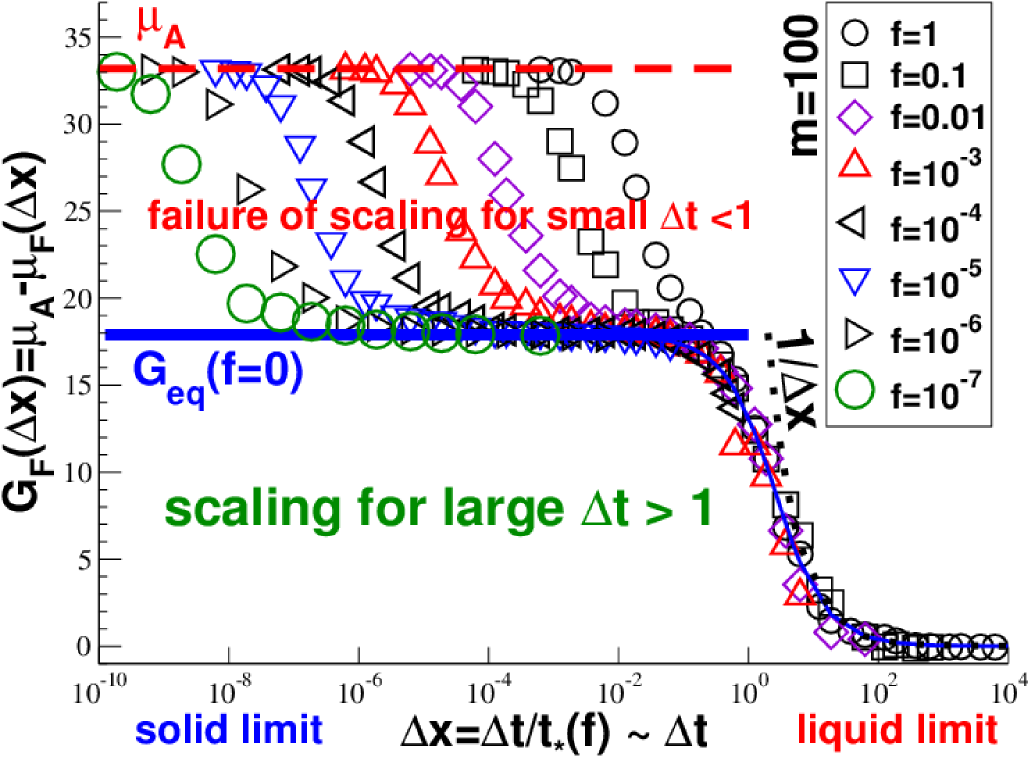
The dimensionless variable $\Delta x=\Delta t/t_{\star}$ has been changed in the main text only as a function of the attempt frequency $f$ while the sampling time $\Delta t$ was kept constant for clarity. The scaling also holds if $\Delta t$ is varied at a constant terminal time $t_{\star}$ as was done for permanent networks Wittmer et al. (2016). As shown in Fig. 10 for the stress-fluctuation formula $G_{\mathrm{F}}$, this assumes that both $\Delta t$ and $t_{\star}(f)$ are sufficiently large. The time average over a sampling time $\Delta t=t_{\mathrm{traj}}=10^{5}$ is replaced by averages over (independent) subintervals of length $\Delta t\leq t_{\mathrm{traj}}$. Note that the largest values of $\Delta x$ indicated in Fig. 10 for each $f$ correspond to the data given in Fig. 5. As expected, all data points collapse on a master curve (thin solid line) as long as $\Delta x$ remains sufficiently large. The data for small $\Delta x$, where the scaling fails, correspond to $\Delta t\ll 1$. This merely shows that the additional time scale $t_{\mathrm{A}}$ (Fig. 6) becomes relevant. Since $\mu_{\mathrm{F}}$ vanishes for small $\Delta t$, this leads to the limit $G_{\mathrm{F}}\to\mu_{\mathrm{A}}$ indicated by the dashed line.

Figure 11: Comparison of $G(t)=\mu_{\mathrm{A}}-h(t)$ and $G_{\mathrm{F}}(\Delta t)\equiv\mu_{\mathrm{A}}-\mu_{\mathrm{F}}(\Delta t)$ for one example in the liquid limit ($f=0.01$, $\Delta x=62.5$). Confirming Eq. (4), $G_{\mathrm{F}}(\Delta t)$ is equivalent to the weighted integral over $G(t)$ indicated by the dotted line. Note that $G(t\approx\Delta t)\approx G_{\mathrm{F}}(\Delta t)$ in the three time regimes where the response modulus has a plateau (shoulder). $G_{\mathrm{F}}(\Delta t)$ is delayed with respect to $G(t)$ due to the strong weight of small times to the integral Eq. (47). The thin solid line indicates Eq. (6).

Appendix F Comparison of $G(t)$ and $G_{\mathrm{F}}(\Delta t)$

Assuming $y(t)$ to be an arbitrary well-behaved function of $t$ let us consider the linear functional

$${\cal P}_{\Delta t}[y(t)]\equiv\frac{2}{\Delta t^{2}}\int_{0}^{\Delta t}\text{d}t\ (\Delta t-t)\ y(t)$$ (47)

motivated by Eq. (4). Note that contributions at the lower boundary of the integral have a strong weight due to the factor $(\Delta t-t)$ and that for a constant function

$$y(t)=c\mbox{ we have }{\cal P}_{\Delta t}[c]=c,$$ (48)

i.e. the $\Delta t$-dependence drops out. This does even hold to leading order if $y(t)\approx c$ only for large $t$ or for a finite $t$-window if this window is sufficiently large. Assuming time translational invariance the shear stress fluctuation $\mu_{\mathrm{F}}(\Delta t)$ is quite generally given by $\mu_{\mathrm{F}}(\Delta t)={\cal P}_{\Delta t}[h(t)]$ Wittmer et al. (2015a); foo (a). Since $\mu_{\mathrm{A}}$ is constant, Eq. (48) and Eq. (1) imply

$$G_{\mathrm{F}}(\Delta t)\equiv\mu_{\mathrm{A}}-\mu_{\mathrm{F}}(\Delta t)={\cal P}_{\Delta t}[G(t)]$$ (49)

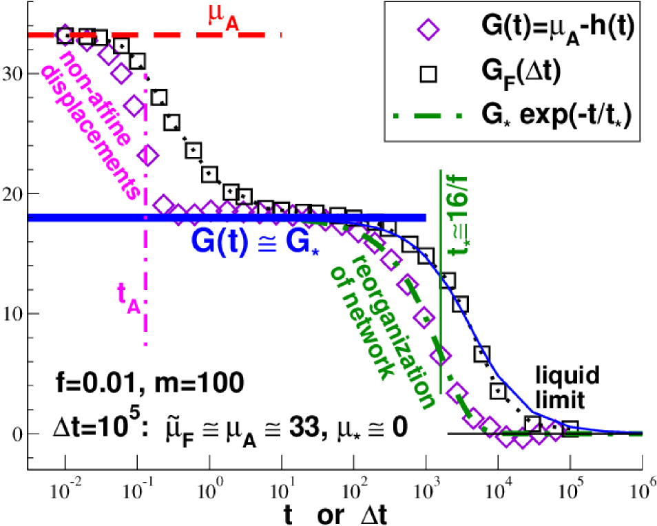
in agreement with Eq. (4). According to Eq. (48), $G_{\mathrm{F}}(\Delta t)$ should become similar to $G(t\approx\Delta t)$ in the three time windows $t\ll t_{\mathrm{A}}$, $t_{\mathrm{A}}\ll t\ll t_{\star}(f)$ and $t_{\star}(f)\ll t$ where $h(t)$ and $G(t)$ become approximatively constant (Fig. 6). This is consistent with the data presented in Fig. 11 for $f=0.01$. Note that specifically $G_{\mathrm{F}}(\Delta t)\approx\mu_{\mathrm{A}}$ for $\Delta t\ll t_{\mathrm{A}}$ in agreement with Fig. 10.

References

- Alexander (1998) S. Alexander, Physics Reports 296, 65 (1998).
- Hansen and McDonald (2006) J. Hansen and I. McDonald, Theory of simple liquids (Academic Press, New York, 2006), 3nd edition.
- Götze (2009) W. Götze, Complex Dynamics of Glass-Forming Liquids: A Mode-Coupling Theory (Oxford University Press, Oxford, 2009).
- de Gennes (1979) P. G. de Gennes, Scaling Concepts in Polymer Physics (Cornell University Press, Ithaca, New York, 1979).
- Doi and Edwards (1986) M. Doi and S. F. Edwards, The Theory of Polymer Dynamics (Clarendon Press, Oxford, 1986).
- Witten and Pincus (2004) T. Witten and P. A. Pincus, Structured Fluids: Polymers, Colloids, Surfactants (Oxford University Press, Oxford, 2004).
- Rubinstein and Colby (2003) M. Rubinstein and R. Colby, Polymer Physics (Oxford University Press, Oxford, 2003).
- Stauffer and Aharnony (1994) D. Stauffer and A. Aharnony, Introduction to percolation theory (Taylor & Francis, London, 1994).
- Ulrich et al. (2006) S. Ulrich, X. Mao, P. Goldbart, and A. Zippelius, Europhysics Lett. 76, 677 (2006).
- Wittmer et al. (2016) J. P. Wittmer, H. Xu, and J. Baschnagel, Phys. Rev. E 93, 012103 (2016).
- Wittmer et al. (2013) J. P. Wittmer, H. Xu, P. Polińska, F. Weysser, and J. Baschnagel, J. Chem. Phys. 138, 12A533 (2013).
- Wittmer et al. (2015a) J. P. Wittmer, H. Xu, and J. Baschnagel, Phys. Rev. E 91, 022107 (2015a).
- Wittmer et al. (2015b) J. P. Wittmer, H. Xu, O. Benzerara, and J. Baschnagel, Mol. Phys. 113, 2881 (2015b).
- Wittmer et al. (2015c) J. P. Wittmer, I. Kriuchevskyi, J. Baschnagel, and H. Xu, Eur. Phys. J. B 88, 242 (2015c).
- Allen and Tildesley (1994) M. Allen and D. Tildesley, Computer Simulation of Liquids (Oxford University Press, Oxford, 1994).
- Lebowitz et al. (1967) J. L. Lebowitz, J. K. Percus, and L. Verlet, Phys. Rev. 153, 250 (1967).
- Barrat et al. (1988) J.-L. Barrat, J.-N. Roux, J.-P. Hansen, and M. L. Klein, Europhys. Lett. 7, 707 (1988).
- Wittmer et al. (2002) J. P. Wittmer, A. Tanguy, J.-L. Barrat, and L. Lewis, Europhys. Lett. 57, 423 (2002).
- Tanguy et al. (2002) A. Tanguy, J. P. Wittmer, F. Leonforte, and J.-L. Barrat, Phys. Rev. B 66, 174205 (2002).
- Flenner and Szamel (2015) E. Flenner and G. Szamel, Phys. Rev. Lett. 107, 105505 (2015).
- Xu et al. (2012) H. Xu, J. Wittmer, P. Polińska, and J. Baschnagel, Phys. Rev. E 86, 046705 (2012).
- Squire et al. (1969) D. R. Squire, A. C. Holt, and W. G. Hoover, Physica 42, 388 (1969).
- Lutsko (1989) J. F. Lutsko, J. Appl. Phys 65, 2991 (1989).
- Mizuno et al. (2013) H. Mizuno, S. Mossa, and J.-L. Barrat, Phys. Rev. E 87, 042306 (2013).
- foo (a) A similar relation exists in polymer theory Doi and Edwards (1986) expressing the radius of gyration of a chain as a weighted integral over internal mean-squared segment sizes.
- foo (b) One may see Eq. (4) as the fundamental definition of the -dependent stress-fluctuation formula. Similar expressions can be formulated for other response functions and associated stress-fluctuation formulae.
- Zilman et al. (2003) A. Zilman, J. Kieffer, F. Molino, G. Porte, and S. A. Safran, Phys. Rev. Lett. 91, 2003 (2003).
- Hed and Safran (2006) G. Hed and S. Safran, Eur. Phys. J. E 19, 69 (2006).
- Testard et al. (2008) V. Testard, J. Oberdisse, and C. Ligoure, Macromolecules 41, 7219 (2008).
- Montarnal et al. (2011) D. Montarnal, M. Capelot, F. Tournilhac, and L. Leibler, Science 334, 965 (2011).
- Smallenburg et al. (2013) F. Smallenburg, L. Leibler, and F. Sciortino, Phys. Rev. Lett. 111, 188002 (2013).
- Roldán-Vargas et al. (2013) S. Roldán-Vargas, F. Smallenburg, W. Kob, and F. Sciortino, J. Chem. Phys. 139, 244910 (2013).
- Tonhauser et al. (2010) C. Tonhauser, D. Wilms, Y. Korth, H. Frey, and C. Friedrich, Macromolecular Rapid Comm. 31, 2127 (2010).
- Berthier et al. (2010) L. Berthier, E. Flenner, H. Jacquin, and G. Szamel, Phys. Rev. E 81, 031505 (2010).
- Berthier et al. (2011) L. Berthier, H. Jacquin, and F. Zamponi, Phys. Rev. E 84, 051103 (2011).
- Wittmer et al. (1998) J. P. Wittmer, A. Milchev, and M. E. Cates, J. Chem. Phys. 109, 834 (1998).
- Huang et al. (2006) C. C. Huang, H. Xu, F. Crevel, J. Wittmer, and J.-P. Ryckaert, in Computer Simulations in Condensed Matter: from Materials to Chemical Biology (Springer, Lect. Notes Phys., International School of Solid State Physics, Berlin/Heidelberg, 2006), vol. 704, pp. 379–418.
- Duering et al. (1991) E. Duering, K. Kremer, and G. S. Grest, Phys. Rev. Lett. 67, 3531 (1991).
- Klix et al. (2012) C. Klix, F. Ebert, F. Weysser, M. Fuchs, G. Maret, and P. Keim, Phys. Rev. Lett. 109, 178301 (2012).
- foo (c) This could be generalized by imposing an energy penalty with being the number of springs per bead. One may, e.g., consider for and , and for all other and in this way generate equilibrium polymer systems Wittmer et al. (1998); Huang et al. (2006) with a few branching points where .
- foo (d) Detailed balance implies that a bond can neither be broken nor created with . Note also that the neighbor list of beads around the pivot monomer contains exactly the same number of possible new sites before and after the hopping of the spring end from monomer to sketched in panel (c) of Fig. 1, i.e. no additional weights are needed to ensure detailed balance Landau and Binder (2000).
- Landau and Binder (2000) D. P. Landau and K. Binder, A Guide to Monte Carlo Simulations in Statistical Physics (Cambridge University Press, Cambridge, 2000).
- foo (e) Assuming time-reversal symmetry this power is expected Wittmer et al. (2015c); Hansen and McDonald (2006). Time-reversal symmetry applies on this time scale since the Langevin thermostat is irrelevant below a time of order .
- foo (f) Equation (23) is merely stated here as a phenomenological description of the data. A theoretical justification will be presented elsewhere.
- foo (g) For convenience, we assume monodisperse particles of unit mass , i.e. particle momenta and velocities are equivalent.
- Goldstein et al. (2001) H. Goldstein, J. Safko, and C. Poole, Classical Mechanics (Addison-Wesley, 2001), 3nd edition.