Explicit solutions for a nonlinear model on the honeycomb and triangular lattices.

Abstract

We study a simple nonlinear model defined on the honeycomb and triangular lattices. We propose a bilinearization scheme for the field equations and demonstrate that the resulting system is closely related to the well-studied integrable models, such as the Hirota bilinear difference equation and the Ablowitz-Ladik system. This result is used to derive the two sets of explicit solutions: the $N$-soliton solutions and ones constructed of the Toeplitz determinants.

2010 Mathematics Subject Classification: 37J35, 11C20, 35C08, 15B05

1 Introduction.

We study a simple nonlinear model defined on the honeycomb and triangular lattices (HL and TL). The main aim of this work is to extend the direct methods of the soliton theory to the case of ‘non-square’, i.e. different from $\mathbb{Z}^{2}$, lattices.

Although there has been considerable interest in the integrable nonlinear models on such lattices (see e.g. [7, 10, 15, 2, 3, 11, 9, 8, 6, 12]) there are still many problems to solve in this field. The main source of difficulties arising in studies of integrable models on the HL and TL is a lack of natural ways to separate variables. This hinders the usage of the standard approaches like, for example, the inverse scattering transform.

There are several strategies to address the non-square lattices. One of them, which was used, in, for example, [7, 10, 15], is to consider the HL and TL as sublattices of sections of the $\mathbb{Z}^{3}$-lattice. In other words, this approach is to consider the model in question as a restriction of a more general (higher dimensional) one. Another approach has been developed in the works of Adler, Bobenko, Suris and co-authors [2, 3, 11, 9, 8, 6, 12] who elaborated a framework for integrable models on non-square lattices and, more generally, on arbitrary graphs. Among different aspects of this approach we would highlight two moments. First, there is an almost algorithmical way to convert an integrable model on a graph that possesses the property of the three-dimensional consistency [4] to the one on the quad-graph [3, 11], i.e. to the system of four-point equations (compare with the system of the discrete Moutard equations from [15]). The second ingredient is the special form of the Lax (or zero-curvature) representation, which is called in [3] the “trivial monodromy representation”. The results of [2, 3, 11, 9, 8, 6, 12] provide answers to many questions arising in the theory of integrable systems. However, if we consider the problem of finding solutions, we have to admit that there is still much work to be done. While in the classical integrable models (on the square lattice, in our case) the zero-curvature representation is a base for the inverse scattering transform which is a tool to derive solutions (at least to linearize the problem), the corresponding methods for models on graphs, that use the trivial monodromy representation, are, so far, to be developed. The possibility to convert an integrable model into the one on the quad-graph is very attracting from the viewpoint of the so-called direct methods. However, a practical implementation of this idea may face some difficulties (we return to this question in section 2.3).

In this work we do not study general aspects of the integrability and the geometry of the HL and TL. We restrict ourselves to the following problem: to find explicit solutions for one of the ‘universal’ integrable models of the paper [3] which was studied in [11]. This model is described in section 2. In section 3, we introduce new variables (the tau-functions), bilinearize the field equations and demonstrate that the resulting system is closely related to the well-studied integrable models, such as the Hirota bilinear difference (or discrete KP) and the Ablowitz-Ladik equations (the important difference between our approach and the one of [15, 11] is that we use, instead of the four-point quad-equations, a system of three-point equations). Then, we present the two sets of explicit solutions for this system that provide the two families of explicit solutions for the equations we want to solve: solutions constructed of the Toeplitz determinants and the $N$-soliton solutions (see section 4 for the case of HL and section 5 for the case of TL).

Of course, during the implementation of this standard program, we meet the manifestations of the peculiar features of the HL and TL. However, as a reader will see, one can overcome the emerging complications by elementary means.

2 Definitions and main equations.

2.1 Honeycomb lattice.

The model that we study in this paper can be defined in terms of the action

$$\mathcal{S}=\sum\limits_{\mathsf{e}\in\mathsf{E}}\mathcal{L}(\mathsf{e})$$ (1)

where $\mathsf{E}=\{\mathsf{e}\}$ is the set of edges of the lattice. The edge function $\mathcal{L}(\mathsf{e})$ depends on variables defined on the set of nodes $\mathsf{V}=\{\mathsf{v}\}$ of the lattice, $\mathcal{L}(\mathsf{e})=\mathcal{L}\left(\mathsf{v}_{+}(\mathsf{e}),\mathsf{v}_{-}(\mathsf{e})\right)$ where $\mathsf{v}_{\pm}(\mathsf{e})$ are the two nodes connected by the edge $\mathsf{e}$ (so, in fact, it is an ‘interaction’ function), and is given by

$$\mathcal{L}(\mathsf{e})=\Gamma(\mathsf{e})\ln\left|u(\mathsf{v}_{+}(\mathsf{e}))-u(\mathsf{v}_{-}(\mathsf{e}))\right|$$ (2)

where $\Gamma(\mathsf{e})$ are constants that depend only on the direction of the edge $\mathsf{e}$, $\Gamma(\mathsf{e})\in\{\Gamma_{1},\Gamma_{2},\Gamma_{3}\}$ (see equation (11) below) and are subjected to the restriction, which appears in [3, 11],

$$\sum_{\mathsf{e}\;(\mathsf{v}\in\mathsf{e})}\Gamma(\mathsf{e})=0,\qquad\mathsf{v}\in\mathsf{V}$$ (3)

(we discuss this restriction in the Conclusion). Here, $u=u(\mathsf{v})$ is a function that should be found from the ‘variational’ equations

$$\left.\partial\mathcal{S}\right/\partial u(\mathsf{v})=0,\qquad\mathsf{v}\in\mathsf{V}.$$ (4)

In what follows, we extensively use the fact that the HL is a bipartite graph. So, from the beginning, we consider its set of vertices $\mathsf{V}$ as a sum of two subsets, which we call ‘positive’ and ‘negative’, $\mathsf{V}=\mathsf{V}^{+}\cup\mathsf{V}^{-}$ (in figure 1, the vertices that belong to $\mathsf{V}^{+}$ are shown by black circles and the vertices that belong to $\mathsf{V}^{-}$ are shown by white ones). Thus, the maps $\mathsf{v}_{\pm}(\mathsf{e})$ are maps to $\mathsf{V}^{\pm}$, $\mathsf{v}_{\pm}:\mathsf{E}\to\mathsf{V}^{\pm}$.

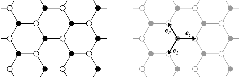
Figure 1: Bipartition of the HL and base vectors.

Hereafter, instead of the $\mathsf{e}$-$\mathsf{v}$ notation, we use the vector one. To this end we introduce coplanar vectors $\bm{e}_{1}$, $\bm{e}_{2}$ and $\bm{e}_{3}$ related by

$$\sum_{i=1}^{3}\bm{e}_{i}=\bm{0}$$ (5)

(see figure 1), the set of lattice vectors $\Lambda$ (positions of the nodes of the HL),

$$\Lambda=\left\{\left.\bm{n}=\sum_{i=1}^{3}n_{i}\bm{e}_{i},\quad n_{i}\in\mathbb{Z}\quad\right|\quad\sum_{i=1}^{3}n_{i}\neq 2\,\mathop{\mbox{mod}}\,3\right\},$$ (6)

which can be decomposed as

$$\Lambda=\Lambda^{+}\cup\Lambda^{-}$$ (7)

with

$$\begin{array}[]{l}\Lambda^{+}=\left\{\left.\bm{n}=\sum\limits_{i=1}^{3}n_{i}\bm{e}_{i},\quad n_{i}\in\mathbb{Z}\quad\right|\quad\sum\limits_{i=1}^{3}n_{i}=0\,\mathop{\mbox{mod}}\,3\;\right\},\\[11.38109pt] \Lambda^{-}=\left\{\left.\bm{n}=\sum\limits_{i=1}^{3}n_{i}\bm{e}_{i},\quad n_{i}\in\mathbb{Z}\quad\right|\quad\sum\limits_{i=1}^{3}n_{i}=1\,\mathop{\mbox{mod}}\,3\;\right\}\end{array}$$ (8)

(the vertex whose position is determined by $\bm{n}\in\Lambda^{\pm}$ belongs to $\mathsf{V}^{\pm}$) and write $u(\bm{n})$ instead of $u(\mathsf{v})$. It should be noted that, first, the usage of the three integer coordinates $n_{i}$ ($i=1,2,3$) does not mean that we are passing to the cubic lattice $\mathbb{Z}^{3}$ and, secondly, that one should be careful and not forget the fact that the decomposition $\bm{n}=\sum_{i=1}^{3}n_{i}\bm{e}_{i}$ is not unique: triples $\left(n_{1},n_{2},n_{3}\right)$ and $\left(n_{1}+N,n_{2}+N,n_{3}+N\right)$ with integer non-zero $N$ define the same vector $\bm{n}$.

In vector terms, the action $\mathcal{S}$ (1) can be presented as

$$\mathcal{S} = \sum\limits_{\bm{n}\in\Lambda^{+}}\sum\limits_{i=1}^{3}\Gamma_{i}\,\ln\left|u(\bm{n})-u(\bm{n}+\bm{e}_{i})\right|$$ (9)

$$= \sum\limits_{\bm{n}\in\Lambda^{-}}\sum\limits_{i=1}^{3}\Gamma_{i}\,\ln\left|u(\bm{n})-u(\bm{n}-\bm{e}_{i})\right|$$ (10)

where we use, instead of $\Gamma(\mathsf{e})$, constants $\Gamma_{i}$,

$$\Gamma(\mathsf{e})=\Gamma_{i}\quad\mbox{if}\quad\mathsf{e}\,\|\,\bm{e}_{i}\quad(i=1,2,3),$$ (11)

(where $\|$ stands for “parallel”) subjected to the restriction (3),

$$\sum\limits_{i=1}^{3}\Gamma_{i}=0.$$ (12)

The ‘variational’ equations (4) can now be written as

$$\sum_{i=1}^{3}\frac{\Gamma_{i}}{u(\bm{n})-u(\bm{n}+\bm{e}_{i})}=0\qquad(\bm{n}\in\Lambda^{+}),$$ (13)

$$\sum_{i=1}^{3}\frac{\Gamma_{i}}{u(\bm{n})-u(\bm{n}-\bm{e}_{i})}=0\qquad(\bm{n}\in\Lambda^{-}).$$ (14)

Namely these equations are the main object of our study.

2.2 Triangular lattice.

It is straightforward to verify that any solution of (13) and (14) is, at the same time, a solution for the field equations of the model similar to (1) and (2) but defined on the TL which is a sublattice of the HL discussed previously.

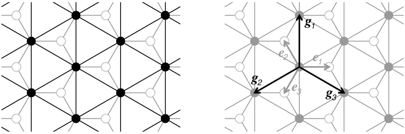
Figure 2: Honeycomb and triangular lattices

Indeed, one can easily derive from (13) and (14) explicit expressions for $u(\bm{n})$ in terms of the values of $u$ at the adjacent points. In other words, we can eliminate, for example, the ‘negative’ vertices,

$$u(\bm{n})=-\frac{\sum_{i=1}^{3}\Gamma_{i}\;u(\bm{n}-\bm{e}_{i-1})u(\bm{n}-\bm{e}_{i+1})}{\sum_{i=1}^{3}\Gamma_{i}\;u(\bm{n}-\bm{e}_{i})}\qquad(\bm{n}\in\Lambda^{-}).$$ (15)

In this equation, as well as in the rest of the paper, we use the following convention: all arithmetic operations with $\bm{e}$- and $\Gamma$-indices are understood modulo $3$,

$$\bm{e}_{i\pm 3}=\bm{e}_{i},\qquad\Gamma_{i\pm 3}=\Gamma_{i}\qquad(i=1,2,3).$$ (16)

Equations (15) and (12) lead to

$$\frac{\Gamma_{i}}{u(\bm{n})-u(\bm{n}+\bm{e}_{i})} = -\frac{\Gamma_{i-1}}{u(\bm{n})-u(\bm{n}+\bm{e}_{i}-\bm{e}_{i+1})}$$ (17)

$$-\frac{\Gamma_{i+1}}{u(\bm{n})-u(\bm{n}+\bm{e}_{i}-\bm{e}_{i-1})}\qquad(\bm{n}\in\Lambda^{+})$$

Now, equation (13) implies

$$\sum_{i=1}^{3}\Gamma_{i}\left[\frac{1}{u(\bm{n})-u(\bm{n}+\bm{g}_{i})}+\frac{1}{u(\bm{n})-u(\bm{n}-\bm{g}_{i})}\right]=0\qquad(\bm{n}\in\Lambda^{+})$$ (18)

where

$$\bm{g}_{1}=\bm{e}_{2}-\bm{e}_{3},\qquad\bm{g}_{2}=\bm{e}_{3}-\bm{e}_{1},\qquad\bm{g}_{3}=\bm{e}_{1}-\bm{e}_{2}$$ (19)

or

$$\bm{g}_{i}=\bm{e}_{i+1}-\bm{e}_{i-1}.$$ (20)

It is easy to see that these equations have the form $\partial\mathcal{S}_{{\!\scriptscriptstyle\triangle}}/\partial u(\bm{n})=0$ with

$$\mathcal{S}_{{\!\scriptscriptstyle\triangle}}=\sum_{\bm{n}\in\Lambda^{+}}\sum_{i=1}^{3}\Gamma_{i}\,\ln\left|u(\bm{n})-u(\bm{n}+\bm{g}_{i})\right|.$$ (21)

Thus, solutions for (13) and (14) solve also the field equations for the model similar to (1) and (2), with the same interaction, only, this time, along the edges of the TL $\Lambda^{+}$ (it is clear that one can repeat the same procedure to arrive at the lattice $\Lambda^{-}$).

2.3 Cross-ratio system.

In this section we discuss the results of [11] and their possible applications to the problem we are going to solve. The authors of [11] developed a general construction that enables to transform a problem on a graph to the system of quad-equations. In particular, they considered a model (which they call “additive rational Toda system”) which is a generalized version of the model discussed in this paper. Briefly, their scheme for the HL can described as follows: we extend our lattice by adding the vertices corresponding to the faces of the HL and consider equations we want to solve on $\Lambda^{ext}=\Lambda\cup\Lambda^{\circ}$, where

$$\Lambda^{\circ}=\left\{\left.\bm{n}=\sum\limits_{i=1}^{3}n_{i}\bm{e}_{i},\quad n_{i}\in\mathbb{Z}\quad\right|\quad\sum\limits_{i=1}^{3}n_{i}=2\mathop{\mbox{mod}}3\;\right\}.$$ (22)

It has been shown that, if one introduce $u(\bm{n})$ with $\bm{n}\in\Lambda^{\circ}$ by the equations

$$\frac{\Gamma_{i}}{u(\bm{n})-u(\bm{n}+\bm{e}_{i})}=\frac{\gamma_{i+1}}{u(\bm{n})-u(\bm{n}-\bm{e}_{i+1})}-\frac{\gamma_{i-1}}{u(\bm{n})-u(\bm{n}-\bm{e}_{i-1})}\qquad(\bm{n}\in\Lambda^{+})$$ (23)

with

$$\Gamma_{i}=\gamma_{i+1}-\gamma_{i-1}\qquad(\gamma_{i\pm 3}=\gamma_{i}),$$ (24)

then $u(\bm{n})$ is a solution for (13) provided it obey the so-called cross-ratio system on $\Lambda^{ext}$,

$$0 = \gamma_{i+1}\left[u(\bm{n}+\bm{e}_{i})-u(\bm{n}-\bm{e}_{i+1})\right]\left[u(\bm{n})-u(\bm{n}-\bm{e}_{i-1})\right]$$ (25)

$$- \gamma_{i-1}\left[u(\bm{n}+\bm{e}_{i})-u(\bm{n}-\bm{e}_{i-1})\right]\left[u(\bm{n})-u(\bm{n}-\bm{e}_{i+1})\right]\qquad(\bm{n}\in\Lambda^{+}).$$

In a similar way, it can be shown that the system

$$0 = \gamma_{i+1}\left[u(\bm{n}-\bm{e}_{i})-u(\bm{n}+\bm{e}_{i+1})\right]\left[u(\bm{n})-u(\bm{n}+\bm{e}_{i-1})\right]$$ (26)

$$- \gamma_{i-1}\left[u(\bm{n}-\bm{e}_{i})-u(\bm{n}+\bm{e}_{i-1})\right]\left[u(\bm{n})-u(\bm{n}+\bm{e}_{i+1})\right]\qquad(\bm{n}\in\Lambda^{-}).$$

implies (14). In both cases, one arrives at the set of the cross-ratio equations

$$\mathfrak{q}_{jk}(\bm{n}) := \gamma_{j}\left[u(\bm{n})-u(\bm{n}+\bm{e}_{k})\right]\left[u(\bm{n}+\bm{e}_{j}+\bm{e}_{k})-u(\bm{n}+\bm{e}_{j})\right]$$ (27)

$$- \gamma_{k}\left[u(\bm{n})-u(\bm{n}+\bm{e}_{j})\right]\left[u(\bm{n}+\bm{e}_{j}+\bm{e}_{k})-u(\bm{n}+\bm{e}_{k})\right]=0$$

where $(j,k)\in\{(1,2),(1,3),(2,3)\}$. Thus, one may try to use the already known solutions for cross-ratio equation to obtain the ones for (13) and (14). However, it turns out to be not a trivial problem. The case is that the cross-ratio system of [11] is not the same that the cross-ratio equation of, for example, [21, 20] or [19, 17]. The latter, is usually understood as an equation on $\mathbb{Z}^{2}$ whereas here, following the construction of [11], we have three types of quadrilaterals and hence three equations with different labelling (in the terminology of [11]). Thus, to use the results of [21, 20, 19, 17] one has either to find common solutions for the all three cross-ratio equations or to find out how to ‘glue together’ solutions for equations with different parameters. This is an interesting problem. which, however, is outside the scope of this paper. Moreover, in what follows we do not exploit the quad-equations approach and use, instead of the cross-ratio equation, another well-known system.

3 Bilinearization of the field equations.

In this section we present the main result of this paper. We bilinearize the field equations (13) and (14) and demonstrate the relationships of the resulting system with the already known integrable models. The procedure that we use is, for the most part, rather standard. However, there are few non-trivial moments that need some additional comments. We formulate some of the key statements ‘as is’, without preliminary motivation, hoping that a reader will find the answers to possible questions in the following proofs and discussion.

We study a two-dimensional lattice. However, we have the three type of translations that correspond to the three vectors $\bm{e}_{i}$. Of course, one can introduce a basis consisting of two vectors and proceed in the standard manner, but, in our opinion, such approach has its disadvantages, most of which stem from the fact that it disregards the symmetry of the problem. Here we use another scheme. We consider our equations as a three-dimensional problem, bearing in mind that at some stage we have to take into account the fact that $\sum_{i=1}^{3}\bm{e}_{i}=\bm{0}$.

The ‘three-dimensionality’ of the equations that we want to solve does not provide insuperable problems: there are some already known integrable systems in dimensions higher than two (see, for example, [5, 16] for the lists of integrable discrete three-dimensional equations) and in what follows we use one of them. The second moment, stemming from the necessity to ensure the triviality of the superposition of the translations corresponding to $\sum_{i=1}^{3}\bm{e}_{i}$, turns out to be more embarrassing: a straightforward application of corresponding restrictions can drastically narrow the family of available solutions (we return to this question in the next sections when discussing the specific solutions). To overcome these difficulties, we ‘replace’ the vectors $\bm{e}_{i}$ with arbitrary vectors $\bm{\alpha}_{i}$,

$$\bm{e}_{i}\to\bm{\alpha}_{i}-\bm{\alpha}_{*},\qquad\bm{\alpha}_{*}=\frac{1}{3}\sum_{i=1}^{3}\bm{\alpha}_{i}$$ (28)

which automatically takes into account (5). In other words, we will consider, instead of $u(\bm{n})$, $\bm{n}=\sum\nolimits_{i=1}^{3}n_{i}\bm{e}_{i}$, functions of $\bm{\nu}=\sum\nolimits_{i=1}^{3}n_{i}\left(\bm{\alpha}_{i}-\bm{\alpha}_{*}\right)$.

Then, we make the substitution

$$u(\bm{n})=\left\{\begin{array}[]{ccl}q(\bm{\nu})&&(\bm{n}\in\Lambda^{+})\\[5.69054pt] \displaystyle-1/r(\bm{\nu}-2\bm{\alpha}_{*})&&(\bm{n}\in\Lambda^{-})\end{array}\right.$$ (29)

and introduce the triplet of the tau-functions $(\sigma,\tau,\rho)$ by

$$q=\frac{\sigma}{\tau},\qquad r=\frac{\rho}{\tau}.$$ (30)

Finally, it can be shown that this construction leads to solutions for our equations (13) and (14) provided $\sigma$, $\tau$, and $\rho$ solve the following bilinear system:

$$\sigma(\bm{\nu}+\bm{\alpha})\tau(\bm{\nu}+\bm{\beta})-\tau(\bm{\nu}+\bm{\alpha})\sigma(\bm{\nu}+\bm{\beta}) = a_{\bm{\alpha},\bm{\beta}}\,\tau(\bm{\nu})\sigma(\bm{\nu}+\bm{\alpha}+\bm{\beta}),$$ (31)

$$\tau(\bm{\nu}+\bm{\alpha})\rho(\bm{\nu}+\bm{\beta})-\rho(\bm{\nu}+\bm{\alpha})\tau(\bm{\nu}+\bm{\beta}) = a_{\bm{\alpha},\bm{\beta}}\,\rho(\bm{\nu})\tau(\bm{\nu}+\bm{\alpha}+\bm{\beta}),$$ (32)

$$\tau(\bm{\nu})\tau(\bm{\nu}+\bm{\alpha}+\bm{\beta})+\rho(\bm{\nu})\sigma(\bm{\nu}+\bm{\alpha}+\bm{\beta}) = b_{\bm{\alpha},\bm{\beta}}\,\tau(\bm{\nu}+\bm{\alpha})\tau(\bm{\nu}+\bm{\beta})$$ (33)

where skew-symmetric constants $a_{\bm{\alpha},\bm{\beta}}$ and symmetric constants $b_{\bm{\alpha},\bm{\beta}}$ are related to $\Gamma_{i}$ by

$$\Gamma_{i}=a_{\bm{\alpha}_{i+1},\bm{\alpha}_{i-1}}b_{\bm{\alpha}_{i+1},\bm{\alpha}_{i-1}}.$$ (34)

Here (and in what follows) we use the convention similar to (16),

$$\bm{\alpha}_{i\pm 3}=\bm{\alpha}_{i}\qquad(i=1,2,3).$$ (35)

The main differences between the original system (13), (14) and system (31)–(33) (except that the latter is bilinear) are the following. First, whereas equations (13) and (14) are defined on the sublattices of the two-dimensional HL ($\Lambda^{+}$ and $\Lambda^{-}$), in (31)–(33) one has to deal with the lattice which is $\mathbb{Z}^{3}$ (the parameters $\bm{\alpha}$ and $\bm{\beta}$ belong to $\{\bm{\alpha}_{1},\bm{\alpha}_{2},\bm{\alpha}_{3}\}$). Secondly, instead of two subsystems ((13) for $\Lambda^{+}$ and (14) for $\Lambda^{-}$) we consider all equations of (31)–(33) as defined on all points of $\mathbb{Z}^{3}$. Thus, whereas the tau-functions $\sigma$ and $\rho$ were introduced in (30) for different sublattices of the HL ($\Lambda^{+}$ and $\Lambda^{-}$ correspondingly), in the framework of (31)–(33) they are parts of the triplet $\{\sigma,\tau,\rho\}$ which is associated with each point of $\mathbb{Z}^{3}$. In other words, we have passed from the bipartite system (13) and (14), which reflects the geometry of the HL, to a translationally-invariant system (31)–(33) which is easier to handle, for example, when one is looking for solutions.

Sometimes, to avoid writing separate formulae for $\Lambda^{+}$ and $\Lambda^{-}$, we will take into account the summand $2\bm{\alpha}_{*}$ in (29) by introducing $\bm{\nu}_{\pm}$,

$$\begin{array}[]{lcl}\bm{\nu}_{+}(\bm{n})=\bm{\nu}(\bm{n})&&(\bm{n}\in\Lambda^{+})\\ \bm{\nu}_{-}(\bm{n})=\bm{\nu}(\bm{n})-2\bm{\alpha}_{*}&&(\bm{n}\in\Lambda^{-})\end{array}$$ (36)

that can be presented as

$$\bm{\nu}_{\pm}\left(\sum_{i=1}^{3}n_{i}\bm{e}_{i}\right)=\sum_{i=1}^{3}\left[n_{i}-\mathcal{N}\left(n_{1},n_{2},n_{3}\right)\right]\bm{\alpha}_{i}$$ (37)

with

$$\mathcal{N}\left(n_{1},n_{2},n_{3}\right)=\left\{\begin{array}[]{lcl}\frac{1}{3}\sum_{i=1}^{3}n_{i}&&(\sum_{i=1}^{3}n_{i}=0\,\mathop{\mbox{mod}}3)\\[5.69054pt] \frac{1}{3}\left(\sum_{i=1}^{3}n_{i}+2\right)&&(\sum_{i=1}^{3}n_{i}=1\,\mathop{\mbox{mod}}3)\end{array}\right.$$ (38)

or, alternatively,

$$\mathcal{N}\left(n_{1},n_{2},n_{3}\right)=\left\lfloor\frac{1}{3}\left(\sum_{i=1}^{3}n_{i}+2\right)\right\rfloor$$ (39)

where $\lfloor...\rfloor$ stands for the floor function (integer part): for any integer $N$ and $0\leqslant\delta<1$, $\lfloor N+\delta\rfloor=N$. Note that the differences $n_{i}-\mathcal{N}\left(n_{1},n_{2},n_{3}\right)$ do not depend on the decomposition of a lattice vector $\bm{n}$ into $\bm{n}=\sum_{i=1}^{3}n_{i}\bm{e}_{i}$.

To summarize, the main result of this paper can be presented as

Proposition 3.1.

Any solution for the bilinear system (31)–(33) with the coefficients that satisfy the restriction (34) provide a solution for the nonlinear HL equations (13) and (14), as well as for the nonlinear TL equations (18), which can be obtained by

$$u(\bm{n})=\left\{\begin{array}[]{ccl}\sigma(\bm{\nu}_{+}(\bm{n}))/\tau(\bm{\nu}_{+}(\bm{n}))&&(\bm{n}\in\Lambda^{+})\\[11.38109pt] -\tau(\bm{\nu}_{-}(\bm{n}))/\rho(\bm{\nu}_{-}(\bm{n}))&&(\bm{n}\in\Lambda^{-})\end{array}\right.$$ (40)

where vectors $\bm{\nu}_{\pm}(\bm{n})$ are defined in (37).

In the following subsections we prove this proposition by demonstrating how equations (31)–(33) ‘help’ us to solve the field equations (13), (14) and (18).

3.1 Solving equations (13).

Let us consider a ‘positive’ vertex, $\bm{n}\in\Lambda^{+}$. It follows from definition (29) that

$$u(\bm{n})=q(\bm{\nu}),\qquad u(\bm{n}+\bm{e}_{i})=-1/r(\bm{\nu}-\bm{\alpha}_{i+1}-\bm{\alpha}_{i-1})$$ (41)

which leads to

$$u(\bm{n})-u(\bm{n}+\bm{e}_{i})=\frac{\tau(\bm{\nu}-\bm{\alpha}_{i+1}-\bm{\alpha}_{i-1})\tau(\bm{\nu})+\rho(\bm{\nu}-\bm{\alpha}_{i+1}-\bm{\alpha}_{i-1})\sigma(\bm{\nu})}{\rho(\bm{\nu}-\bm{\alpha}_{i+1}-\bm{\alpha}_{i-1})\tau(\bm{\nu})}.$$ (42)

Equation (33) factorizes the numerator,

$$u(\bm{n})-u(\bm{n}+\bm{e}_{i})=b_{\bm{\alpha}_{i+1},\bm{\alpha}_{i-1}}\frac{\tau(\bm{\nu}-\bm{\alpha}_{i+1})\tau(\bm{\nu}-\bm{\alpha}_{i-1})}{\rho(\bm{\nu}-\bm{\alpha}_{i+1}-\bm{\alpha}_{i-1})\tau(\bm{\nu})},$$ (43)

which leads, together with (34) and (32), to

$$\frac{\Gamma_{i}}{u(\bm{n})-u(\bm{n}+\bm{e}_{i})}=r(\bm{\nu}-\bm{\alpha}_{i+1})-r(\bm{\nu}-\bm{\alpha}_{i-1}).$$ (44)

Now, it is clear that the summation over $i=1,2,3$ yields (13).

This proves that any solution of (31)–(34) provides a solution for (13).

3.2 Solving equations (14).

In a similar way one can demonstrate that system (31)–(33) yields solutions for (14). For any $\bm{n}\in\Lambda^{-}$,

$$u(\bm{n})=-1/r(\bm{\nu}^{\prime}),\qquad u(\bm{n}-\bm{e}_{i})=q(\bm{\nu}^{\prime}+\bm{\alpha}_{i+1}+\bm{\alpha}_{i-1})\qquad(\bm{\nu}^{\prime}=\bm{\nu}_{-}(\bm{n}))$$ (45)

and

$$u(\bm{n})-u(\bm{n}-\bm{e}_{i})=-\frac{\tau(\bm{\nu}^{\prime})\tau(\bm{\nu}^{\prime}+\bm{\alpha}_{i+1}+\bm{\alpha}_{i-1})+\rho(\bm{\nu}^{\prime})\sigma(\bm{\nu}^{\prime}+\bm{\alpha}_{i+1}+\bm{\alpha}_{i-1})}{\rho(\bm{\nu}^{\prime})\tau(\bm{\nu}^{\prime}+\bm{\alpha}_{i+1}+\bm{\alpha}_{i-1})}.$$ (46)

After application of (33) and (32) the above equation leads to

$$u(\bm{n})-u(\bm{n}-\bm{e}_{i})=-b_{\bm{\alpha}_{i+1},\bm{\alpha}_{i-1}}\frac{\tau(\bm{\nu}^{\prime}+\bm{\alpha}_{i+1})\tau(\bm{\nu}^{\prime}+\bm{\alpha}_{i-1})}{\rho(\bm{\nu}^{\prime})\tau(\bm{\nu}^{\prime}+\bm{\alpha}_{i+1}+\bm{\alpha}_{i-1})}$$ (47)

and

$$\frac{\Gamma_{i}}{u(\bm{n})-u(\bm{n}-\bm{e}_{i})}=r(\bm{\nu}^{\prime}+\bm{\alpha}_{i+1})-r(\bm{\nu}^{\prime}+\bm{\alpha}_{i-1})$$ (48)

which demonstrates that $u(\bm{n})$ solves (14), i.e. that any solution of (31)–(34) provides a solution for (14).

3.3 Solving equations (18).

To conclude this section we give another proof of the fact that the proposed construction (29)–(34) provides solutions for equations (18) for the TL.

For any $\bm{n}\in\Lambda^{+}$,

$$u(\bm{n})=q(\bm{\nu}),\qquad u(\bm{n}+\bm{g}_{i})=q(\bm{\nu}+\bm{\alpha}_{i+1}-\bm{\alpha}_{i-1})$$ (49)

and

$$u(\bm{n})-u(\bm{n}+\bm{g}_{i})=\frac{\sigma(\bm{\nu})\tau(\bm{\nu}+\bm{\alpha}_{i+1}-\bm{\alpha}_{i-1})-\tau(\bm{\nu})\sigma(\bm{\nu}+\bm{\alpha}_{i+1}-\bm{\alpha}_{i-1})}{\tau(\bm{\nu})\tau(\bm{\nu}+\bm{\alpha}_{i+1}-\bm{\alpha}_{i-1})}$$ (50)

which, with the help of (31), can be rewritten as

$$u(\bm{n})-u(\bm{n}+\bm{g}_{i})=-a_{\bm{\alpha}_{i+1},\bm{\alpha}_{i-1}}\frac{\sigma(\bm{\nu}+\bm{\alpha}_{i+1})\tau(\bm{\nu}-\bm{\alpha}_{i-1})}{\tau(\bm{\nu})\tau(\bm{\nu}+\bm{\alpha}_{i+1}-\bm{\alpha}_{i-1})}.$$ (51)

This, together with (33), leads to

$$\frac{\Gamma_{i}}{u(\bm{n})-u(\bm{n}+\bm{g}_{i})}=-q^{-1}(\bm{\nu}+\bm{\alpha}_{i+1})-r(\bm{\nu}-\bm{\alpha}_{i-1})$$ (52)

and then to

$$\frac{\Gamma_{i}}{u(\bm{\nu})-u(\bm{n}+\bm{g}_{i})}+\frac{\Gamma_{i}}{u(\bm{\nu})-u(\bm{n}-\bm{g}_{i})}=w_{i+1}(\bm{\nu})-w_{i-1}(\bm{\nu})$$ (53)

where

$$w_{i}(\bm{\nu})=r(\bm{\nu}-\bm{\alpha}_{i})-q^{-1}(\bm{\nu}+\bm{\alpha}_{i}).$$ (54)

Again, the structure of the summand in (18) exposed in (53) leads to the fact that the summation over $i$ produces zero result. This proves that any solution of (31)–(34) provides a solution for (18).

3.4 Möbius invariance.

Another interesting fact that has not been mentioned yet, is the invariance of the field equations for HL or TL with respect to the Möbius transformations:

Proposition 3.2.

If $u(\bm{n})$ solves (13) and (14), or (18), so does

$$\frac{a\,u(\bm{n})+b}{c\,u(\bm{n})+d}$$ (55)

with constant $a$, $b$, $c$ and $d$, $ad-bc\neq 0$.

The proof of this statement is straightforward and is not presented here.

Thus, one can add three arbitrary constants to any solution presented in the following sections.

4 Exact solutions for the HL.

In this section we discuss system (31)–(33) and then present the two sets of exact solutions for the field equations (13) and (14) which are obtained by modification of the already known ones that have been derived for (31)–(33).

4.1 Ablowitz-Ladik-Hirota system.

Here, we collect some known facts about the system (31)–(33), which we write now as

$$0 = a_{\alpha,\beta}\tau\left(\mathop{\mathbb{T}_{\alpha\beta}}{\sigma}\right)-\left(\mathop{\mathbb{T}_{\alpha}}{\sigma}\right)\left(\mathop{\mathbb{T}_{\beta}}{\tau}\right)+\left(\mathop{\mathbb{T}_{\alpha}}{\tau}\right)\left(\mathop{\mathbb{T}_{\beta}}{\sigma}\right),$$ (56)

$$0 = a_{\alpha,\beta}\rho\left(\mathop{\mathbb{T}_{\alpha\beta}}{\tau}\right)-\left(\mathop{\mathbb{T}_{\alpha}}{\tau}\right)\left(\mathop{\mathbb{T}_{\beta}}{\rho}\right)+\left(\mathop{\mathbb{T}_{\alpha}}{\rho}\right)\left(\mathop{\mathbb{T}_{\beta}}{\tau}\right),$$ (57)

$$0 = b_{\alpha,\beta}\left(\mathop{\mathbb{T}_{\alpha}}{\tau}\right)\left(\mathop{\mathbb{T}_{\beta}}{\tau}\right)-\tau\left(\mathop{\mathbb{T}_{\alpha\beta}}{\tau}\right)-\rho\left(\mathop{\mathbb{T}_{\alpha\beta}}{\sigma}\right)$$ (58)

where we use the ‘abstract shift’ notation. Further, we recall that the shifts $\mathbb{T}_{\alpha}$ are, in our case, a way to write the translations $\mathbb{T}_{\alpha}:f(\bm{\nu})\to f(\bm{\nu}+\bm{\alpha})$ and identify the parameters $\alpha$ with the vectors $\bm{\alpha}_{i}$. However, now we want to present some simple, algebraic, consequences of system (56)–(58) which do not depend on the origin of these equations and the ‘inner structure’ of the tau-functions. Thus, one can think of (56)–(58) as a system of difference (or functional) equations with arbitrary, save the consistency restriction that we discuss below (see (65)), skew-symmetric functions $a_{\alpha,\beta}$ and symmetric functions $b_{\alpha,\beta}$ of arbitrary (scalar or vector) parameters $\alpha$ and $\beta$.

It can be shown that an immediate consequence of, say, (57) is the fact that $\tau$ solves the famous Hirota bilinear difference equation (HBDE) [18], also known as the discrete KP equation:

$$0=a_{\alpha,\beta}\left(\mathop{\mathbb{T}_{\gamma}}{\tau}\right)\left(\mathop{\mathbb{T}_{\alpha\beta}}{\tau}\right)-a_{\alpha,\gamma}\left(\mathop{\mathbb{T}_{\beta}}{\tau}\right)\left(\mathop{\mathbb{T}_{\alpha\gamma}}{\tau}\right)+a_{\beta,\gamma}\left(\mathop{\mathbb{T}_{\alpha}}{\tau}\right)\left(\mathop{\mathbb{T}_{\beta\gamma}}{\tau}\right)$$ (59)

(we prove this statement in appendix A.1). Moreover, it turns out that functions $\sigma$ and $\rho$ also solve (59),

$$0=a_{\alpha,\beta}\left(\mathop{\mathbb{T}_{\gamma}}{\omega}\right)\left(\mathop{\mathbb{T}_{\alpha\beta}}{\omega}\right)-a_{\alpha,\gamma}\left(\mathop{\mathbb{T}_{\beta}}{\omega}\right)\left(\mathop{\mathbb{T}_{\alpha\gamma}}{\omega}\right)+a_{\beta,\gamma}\left(\mathop{\mathbb{T}_{\alpha}}{\omega}\right)\left(\mathop{\mathbb{T}_{\beta\gamma}}{\omega}\right),\quad\omega=\sigma,\rho$$ (60)

(see appendix A.1). Thus, equation (57), or (56), can be viewed as the linear problem (or the so-called Lax representation) for the HBDE (see, e.g., [13, 14, 22, 29, 24]). On the other hand, another consequences of equations (56) and (57),

$$0 = a_{\alpha,\beta}\left(\mathop{\mathbb{T}_{\gamma}}{\tau}\right)\left(\mathop{\mathbb{T}_{\alpha\beta}}{\sigma}\right)-a_{\alpha,\gamma}\left(\mathop{\mathbb{T}_{\beta}}{\tau}\right)\left(\mathop{\mathbb{T}_{\alpha\gamma}}{\sigma}\right)+a_{\beta,\gamma}\left(\mathop{\mathbb{T}_{\alpha}}{\tau}\right)\left(\mathop{\mathbb{T}_{\beta\gamma}}{\sigma}\right),$$ (61)

$$0 = a_{\alpha,\beta}\left(\mathop{\mathbb{T}_{\gamma}}{\rho}\right)\left(\mathop{\mathbb{T}_{\alpha\beta}}{\tau}\right)-a_{\alpha,\gamma}\left(\mathop{\mathbb{T}_{\beta}}{\rho}\right)\left(\mathop{\mathbb{T}_{\alpha\gamma}}{\tau}\right)+a_{\beta,\gamma}\left(\mathop{\mathbb{T}_{\alpha}}{\rho}\right)\left(\mathop{\mathbb{T}_{\beta\gamma}}{\tau}\right)$$ (62)

(see appendix A.2 for a proof), can be interpreted as describing the Bäcklund transformations

$$\mbox{BT}_{\mbox{\tiny HBDE}}:\qquad\sigma\stackrel{{\scriptstyle(\ref{alh-bt-st})}}{{\longrightarrow}}\tau\stackrel{{\scriptstyle(\ref{alh-bt-tr})}}{{\longrightarrow}}\rho$$ (63)

between different solutions for the HBDE (note that this chain can be continued in both directions, $...\to\sigma\to\tau\to\rho\to...$ via the extended version of (56) and (57)).

Clearly, one can derive a great number of identities for the functions that satisfy (56) and (57). Here, we write down only one example,

$$A_{\alpha,\beta,\gamma}\tau\left(\mathop{\mathbb{T}_{\alpha\beta\gamma}}{\sigma}\right)=a_{\beta,\gamma}\left(\mathop{\mathbb{T}_{\alpha}}{\sigma}\right)\left(\mathop{\mathbb{T}_{\beta\gamma}}{\tau}\right)-a_{\alpha,\gamma}\left(\mathop{\mathbb{T}_{\beta}}{\sigma}\right)\left(\mathop{\mathbb{T}_{\alpha\gamma}}{\tau}\right)+a_{\alpha,\beta}\left(\mathop{\mathbb{T}_{\gamma}}{\sigma}\right)\left(\mathop{\mathbb{T}_{\alpha\beta}}{\tau}\right)$$ (64)

with $A_{\alpha,\beta,\gamma}=a_{\alpha,\beta}a_{\alpha,\gamma}a_{\beta,\gamma}$ which may be useful, if one wants to demonstrate the so-called three-dimensional consistency of (56) and (57) (see appendix A.3).

Till now, we have considered only the first two equations of the (56)–(58). The last one can be viewed in the framework of the theory of the HBDE as a nonlinear restriction, which is compatible with (56) and (57) provided the constants $a_{\alpha,\beta}$ and $b_{\alpha,\beta}$ met the following condition:

$$a_{\alpha,\beta}b_{\alpha,\beta}-a_{\alpha,\gamma}b_{\alpha,\gamma}+a_{\beta,\gamma}b_{\beta,\gamma}=0$$ (65)

which is derived in appendix A.4.

It turns out that the restricted system (31)–(33) is closely related to another integrable model, which is even ‘older’ than the HBDE: equations (31)–(33) describe the so-called Miwa shifts of the Ablowitz-Ladik hierarchy (ALH) [1].

Indeed, as is demonstrated in B, the functions

$$Q=\frac{E}{b_{\kappa,\kappa}}\frac{\mathop{\mathbb{T}_{\kappa}}{\sigma}}{\tau},\qquad R=\frac{1}{E}\frac{\mathbb{T}_{\kappa}^{-1}\rho}{\tau}$$ (66)

where $E$ is defined by

$$\mathop{\mathbb{T}_{\alpha}}{E}=\frac{1}{b_{\alpha,\kappa}}\;E$$ (67)

satisfy, for a fixed value of $\kappa$,

$$\mathbb{E}_{\alpha}Q-Q = \xi_{\alpha}\left[1-R\left(\mathbb{E}_{\alpha}Q\right)\right]\left(\mathop{\mathbb{T}_{\alpha}}{Q}\right)$$ (68)

$$R-\mathbb{E}_{\alpha}R = \xi_{\alpha}\left[1-R\left(\mathbb{E}_{\alpha}Q\right)\right]\mathbb{T}_{\kappa}^{-1}R$$ (69)

where $\mathbb{E}_{\alpha}=\mathbb{T}_{\alpha}\mathbb{T}_{\kappa}^{-1}$ and $\xi_{\alpha}=a_{\alpha,\kappa}b_{\alpha,\kappa}$. Introducing the $n$-dependence by

$$Q_{n}=\mathbb{T}_{\kappa}^{n}Q,\qquad R_{n}=\mathbb{T}_{\kappa}^{-n}R$$ (70)

one can rewrite (68) and (69) as

$$\mathbb{E}_{\alpha}Q_{n}-Q_{n} = \xi_{\alpha}\left[1-R_{n}\left(\mathbb{E}_{\alpha}Q_{n}\right)\right]\mathbb{E}_{\alpha}Q_{n+1},$$ (71)

$$R_{n}-\mathbb{E}_{\alpha}R_{n} = \xi_{\alpha}\left[1-R_{n}\left(\mathbb{E}_{\alpha}Q_{n}\right)\right]R_{n-1}.$$ (72)

These equations are nothing but the so-called functional representation of the positive flows of the ALH [25, 26]: if we consider $Q_{n}$ and $R_{n}$ as functions of an infinite number of variables, $Q_{n}=Q_{n}\left(z_{m}\right)_{m=1,...,\infty}$, $R_{n}=R_{n}\left(z_{m}\right)_{m=1,...,\infty}$ and identify the shifts $\mathbb{E}_{\alpha}$ with the Miwa shifts,

$$\mathbb{E}_{\alpha}F_{n}\left(z_{m}\right)_{m=1,...,\infty}=F_{n}\left(z_{m}+i\xi_{\alpha}^{m}/m\right)_{m=1,...,\infty},$$ (73)

then equations (71) and (72) can be viewed as an infinite set of differential equation, the simplest of which are given by

$$i\left.\partial Q_{n}\right/\partial z_{1} = \left[1-Q_{n}R_{n}\right]Q_{n+1},$$ (74)

$$-i\left.\partial R_{n}\right/\partial z_{1} = \left[1-Q_{n}R_{n}\right]R_{n-1}$$ (75)

(the complex version of the discrete nonlinear Schrödinger equation). This infinite set of differential equation is the positive part of the ALH. We do not discuss here the negative ALH, whose equations as well can be ‘derived’ from (56)–(58), referring to, for example, section 6 of [27] for details. What is important for our present study is that the ALH (and hence the system (56)–(58)) is an integrable model, which during its 40-year history have attracted considerable interest and which is one of the best-studied integrable systems.

Thus, one can use various results that have been obtained for the HBDE and the ALH to derive solutions for (31)–(33) and hence for system (13) and (14). Namely this approach is used in the following sections where we present two types of solutions: solution built of the Toeplitz determinants and the soliton solutions.

4.2 Toeplitz solutions for the HL.

Here, we presents solutions for our field equations, constructed of the determinants of the Toeplitz matrices $\mathsf{A}^{m}_{\ell}$, defined by

$$\mathsf{A}^{m}_{\ell}=\det\left|\omega_{m-a+b}\right|_{a,b=1,...,\ell}\qquad(\ell\geqslant 1)$$ (76)

and $\mathsf{A}^{m}_{0}=1$. It can be shown that these determinants satisfy the following identities:

$$(\xi-\eta)\mathsf{A}^{m+1}_{\ell+1}\left(\mathop{\mathbb{T}_{\xi\eta}}{\mathsf{A}^{m}_{\ell}}\right)=\left(\mathop{\mathbb{T}_{\xi}}{\mathsf{A}^{m}_{\ell}}\right)\left(\mathop{\mathbb{T}_{\eta}}{\mathsf{A}^{m+1}_{\ell+1}}\right)-\left(\mathop{\mathbb{T}_{\xi}}{\mathsf{A}^{m+1}_{\ell+1}}\right)\left(\mathop{\mathbb{T}_{\eta}}{\mathsf{A}^{m}_{\ell}}\right)$$ (77)

and

$$\left(\mathop{\mathbb{T}_{\xi}}{\mathsf{A}^{m}_{\ell}}\right)\left(\mathop{\mathbb{T}_{\eta}}{\mathsf{A}^{m}_{\ell}}\right)=\mathsf{A}^{m}_{\ell}\left(\mathop{\mathbb{T}_{\xi\eta}}{\mathsf{A}^{m}_{\ell}}\right)+\mathsf{A}^{m+1}_{\ell+1}\left(\mathop{\mathbb{T}_{\xi\eta}}{\mathsf{A}^{m-1}_{\ell-1}}\right)$$ (78)

with shifts $\mathbb{T}_{\zeta}$ being defined by $\mathop{\mathbb{T}_{\zeta}}{\mathsf{A}^{m}_{\ell}}=\det\left|\mathop{\mathbb{T}_{\zeta}}{\omega_{m-a+b}}\right|_{a,b=1,...,\ell}$ where

$$\mathop{\mathbb{T}_{\zeta}}{\omega_{m}}=\omega_{m+1}-\zeta\omega_{m}.$$ (79)

We present, in C, a sketch of a proof of these identities which is based on the results from [28].

It is easy to see from (77) and (78) that tau-functions defined by

$$\sigma=\mathsf{A}^{m-1}_{\ell-1},\quad\tau=\mathsf{A}^{m}_{\ell},\quad\rho=\mathsf{A}^{m+1}_{\ell+1}\qquad(\ell,m=\mbox{constant})$$ (80)

solve equations similar to (56)–(58) with $a_{\xi,\eta}=\xi-\eta$ and $b_{\xi,\eta}=1$,

$$(\xi-\eta)\tau\left(\mathop{\mathbb{T}_{\xi\eta}}{\sigma}\right) = \left(\mathop{\mathbb{T}_{\xi}}{\sigma}\right)\left(\mathop{\mathbb{T}_{\eta}}{\tau}\right)-\left(\mathop{\mathbb{T}_{\eta}}{\sigma}\right)\left(\mathop{\mathbb{T}_{\xi}}{\tau}\right),$$ (81)

$$(\xi-\eta)\rho\left(\mathop{\mathbb{T}_{\xi\eta}}{\tau}\right) = \left(\mathop{\mathbb{T}_{\xi}}{\tau}\right)\left(\mathop{\mathbb{T}_{\eta}}{\rho}\right)-\left(\mathop{\mathbb{T}_{\eta}}{\tau}\right)\left(\mathop{\mathbb{T}_{\xi}}{\rho}\right),$$ (82)

$$\left(\mathop{\mathbb{T}_{\xi}}{\tau}\right)\left(\mathop{\mathbb{T}_{\eta}}{\tau}\right) = \tau\left(\mathop{\mathbb{T}_{\xi\eta}}{\tau}\right)+\rho\left(\mathop{\mathbb{T}_{\xi\eta}}{\sigma}\right).$$ (83)

Thus, one can obtain solutions for our equations by identifying the translations by vectors $\bm{\alpha}_{i}$ with the shifts $\mathbb{T}_{\alpha_{i}}$ where $\{\alpha_{i}\}_{i=1..3}$ is a set of parameters. To write the final formulae, it is convenient to use the $n_{i}$-representation of the lattice vectors and the ‘Fourier’ representation of the functions $\omega_{m}$,

$$\omega_{m}=\int\nolimits_{\gamma}dh\,\hat{\omega}(h)\;h^{m}$$ (84)

with arbitrary contour $\gamma$ and function $\hat{\omega}(h)$. The definition (79) of the shift $\mathbb{T}_{\zeta}$ can be rewritten as

$$\mathop{\mathbb{T}_{\zeta}}{\omega_{m}}=\int\nolimits_{\gamma}dh\,\hat{\omega}(h)\left(h-\zeta\right)h^{m}$$ (85)

and can be extended, using (37), to

$$\omega_{m}(\bm{n})=\int\nolimits_{\gamma}dh\,\hat{\omega}(h,\bm{n})\;h^{m}$$ (86)

with

$$\hat{\omega}(h,\bm{n})=\hat{\omega}(h)\;\prod_{i=1}^{3}\left(h-\alpha_{i}\right)^{n_{i}-\mathcal{N}\left(n_{1},n_{2},n_{3}\right)}\qquad\biggl{(}\bm{n}=\sum_{i=1}^{3}n_{i}\bm{e}_{i}\biggr{)}$$ (87)

and $\mathcal{N}\left(n_{1},n_{2},n_{3}\right)$ being defined in (39).

Gathering the above formulae and making simple modifications, like setting $m=0$ (note that the factor $h^{m}$ can be incorporated into the definition of $\hat{\omega}(h)$) and introducing determinants $\mathsf{D}_{k}$ instead of $\mathsf{A}^{m+k}_{\ell+k}$, we can formulate the following

Proposition 4.1.

The Toeplitz solutions for the nonlinear HL equations (13)–(14) are given by

$$u(\bm{n})=\epsilon\left[\frac{\mathsf{D}_{-\epsilon}(\bm{n})}{\mathsf{D}_{0}(\bm{n})}\right]^{\epsilon}\qquad(\bm{n}\in\Lambda^{\epsilon})$$ (88)

where $\epsilon=\pm 1$, $\Lambda^{\pm 1}=\Lambda^{\pm}$,

$$\mathsf{D}_{k}(\bm{n})=\left\{\begin{array}[]{lcl}\det\left|\omega_{k-a+b}(\bm{n})\right|_{a,b=1,...,\ell+k}&&(\ell+k\geqslant 1)\\ 1&&(\ell+k=0)\end{array}\right.\qquad k=0,\pm 1$$ (89)

and

$$\omega_{m}(\bm{n})=\int\nolimits_{\gamma}dh\,\hat{\omega}(h)\;h^{m}\,\prod_{i=1}^{3}\left(h-\alpha_{i}\right)^{n_{i}-\mathcal{N}\left(n_{1},n_{2},n_{3}\right)}\qquad\biggl{(}\bm{n}=\sum_{i=1}^{3}n_{i}\bm{e}_{i}\biggr{)}$$ (90)

with arbitrary positive integer $\ell$, parameters $\alpha_{i}$ ($i=1,2,3$), contour $\gamma$ and function $\hat{\omega}(h)$, and $\mathcal{N}\left(n_{1},n_{2},n_{3}\right)$ being defined in (39).

Here, we would like to make a comment about the role of the construction (28). One can repeat the calculations of this section without introducing the vectors $\bm{\alpha}_{i}$ and using the shifts $\mathbb{T}_{\varepsilon_{i}}$ describing the ‘original’ translations $f(\bm{n})\to f(\bm{n}+\bm{e}_{i})$. This leads to the relations (90) of proposition 4.1 with $\alpha_{i}$ replaced with $\varepsilon_{i}$ and $\mathcal{N}=0$. However, the restriction $\prod_{i}\mathbb{T}_{\varepsilon_{i}}=1$ implies $\prod_{i}\left(h-\varepsilon_{i}\right)=1$ which means that the integral in (90) is reduced to the sum over the three roots of the cubic equation. Clearly, this family of solutions is noticeably less rich than the one presented above.

4.3 Soliton solutions for the HL.

To derive the $N$-soliton solutions for our model we use the results of [27] where we have presented a large number of identities (soliton Fay identities) for the matrices of a special type. These $N{\times}N$ matrices are defined by

$$\begin{array}[]{lcl}\mathsf{L}\mathsf{A}-\mathsf{A}\mathsf{R}&=&|\,1\,\rangle\langle\,a\,|,\\ \mathsf{R}\mathsf{B}-\mathsf{B}\mathsf{L}&=&|\,1\,\rangle\langle\,b\,|\end{array}$$ (91)

where $\mathsf{L}$ and $\mathsf{R}$ are diagonal constant $N{\times}N$ matrices, $|\,1\,\rangle$ is the $N$-column with all components equal to $1$, $\langle\,a\,|$ and $\langle\,b\,|$ are $N$-component rows that usually depend on the coordinates describing the model (note that we have replaced the $N$-columns $|\,\alpha\,\rangle$ and $|\,\beta\,\rangle$ used in [27] with $|\,1\,\rangle$, which can be done by means of the simple gauge transform).

In [27], the soliton Fay identities are formulated in terms of the shifts defined by

$$\begin{array}[]{lcl}\mathop{\mathbb{T}_{\xi}}{\langle\,a\,|}&=&\langle\,a\,|\left(\mathsf{R}-\xi\right)^{-1},\\[5.69054pt] \mathop{\mathbb{T}_{\xi}}{\langle\,b\,|}&=&\langle\,b\,|\left(\mathsf{L}-\xi\right)\end{array}$$ (92)

which determine the shifts of all other objects (the matrices $\mathsf{A}$ and $\mathsf{B}$, their determinants, the tau-functions constructed of $\mathsf{A}$ and $\mathsf{B}$ etc).

The soliton tau-functions have been defined in [27] as

$$\tau=\det\left|\mathsf{1}+\mathsf{A}\mathsf{B}\right|$$ (93)

and

$$\begin{array}[]{lcl}\sigma&=&\tau\langle\,a\,|(\mathsf{1}+\mathsf{B}\mathsf{A})^{-1}|\,1\,\rangle,\\[5.69054pt] \rho&=&\tau\langle\,b\,|(\mathsf{1}+\mathsf{A}\mathsf{B})^{-1}|\,1\,\rangle\end{array}$$ (94)

The simplest soliton Fay identities, which are equations (3.12)–(3.14) of [27], are exactly equations (33) with $b_{\xi,\eta}=1$ and (31)–(32) with $a_{\xi,\eta}=\xi-\eta$.

Thus, to obtain the $N$-soliton solutions one only needs to introduce the $\bm{n}$-dependence of the matrices $\mathsf{A}$ and $\mathsf{B}$ as well as of the rows $\langle\,a\,|$ and $\langle\,b\,|$, which can be done by (37) and the identification of the translations by vectors $\bm{\alpha}_{i}$ with the shifts $\mathbb{T}_{\alpha_{i}}$ ($i=1,2,3$):

$$\begin{array}[]{lcl}\mathsf{A}(\bm{n})&=&\mathsf{A}_{0}\prod_{i=1}^{3}\left(\mathsf{R}-\alpha_{i}\right)^{\mathcal{N}\left(n_{1},n_{2},n_{3}\right)-n_{i}}\\[5.69054pt] \mathsf{B}(\bm{n})&=&\mathsf{B}_{0}\prod_{i=1}^{3}\left(\mathsf{L}-\alpha_{i}\right)^{n_{i}-\mathcal{N}\left(n_{1},n_{2},n_{3}\right)}\end{array}$$ (95)

with constant matrices $\mathsf{A}_{0}$ and $\mathsf{B}_{0}$ (that are, in fact, $\mathsf{A}(\bm{0})$ and $\mathsf{B}(\bm{0})$) and similar formulae for $\langle\,a(\bm{n})\,|$ and $\langle\,b(\bm{n})\,|$.

After expressing, from (91), $\mathsf{A}_{0}$ and $\mathsf{B}_{0}$ in terms of $\langle\,a_{0}\,|=\langle\,a(\bm{0})\,|$ and $\langle\,b_{0}\,|=\langle\,b(\bm{0})\,|$ one can write the resulting formulae as follows:

Proposition 4.2.

The $N$-soliton solutions for the nonlinear HL equations (13)–(14) are given by

$$u(\bm{n})=\langle\,c_{\pm}\,|\left[\mathsf{A}^{\mp 1}(\bm{n})+\mathsf{B}^{\pm 1}(\bm{n})\right]^{-1}|\,1\,\rangle^{\pm 1}\qquad(\bm{n}\in\Lambda^{\pm}).$$ (96)

where the matrices $\mathsf{A}(\bm{n})$ and $\mathsf{B}(\bm{n})$ are defined in (95) with

$$\mathsf{A}_{0}=\left(\frac{a_{0k}}{L_{j}-R_{k}}\right)_{j,k=1,...,N},\qquad\mathsf{B}_{0}=\left(\frac{b_{0k}}{R_{j}-L_{k}}\right)_{j,k=1,...,N}$$ (97)

and the constant N-rows $\langle\,c_{\pm}\,|$ are given by $\langle\,c_{+}\,|=\langle\,1\,|\mathsf{C}$ and $\langle\,c_{-}\,|=\langle\,1\,|\mathsf{C}^{T}$ (the superscript ‘T’ stands for the transposition) with

$$\mathsf{C}=\mathsf{M}^{-1},\qquad\mathsf{M}=\left(\frac{1}{L_{j}-R_{k}}\right)_{j,k=1,...,N}.$$ (98)

Here, constants $\alpha_{i}$ ($i=1,2,3$), $L_{k}$, $R_{k}$, $a_{0k}$ and $b_{0k}$ ($k=1,...,N$) are the parameters describing the solution.

Again, as in section 4.2, we would like to note that using the main result of this paper, formulated in proposition 3.1, without introducing the $\bm{\alpha}$-vectors (see (28)) one arrives at the restrictions $\prod_{i=1}^{3}\left(\mathsf{L}-\varepsilon_{i}\right)=\prod_{i=1}^{3}\left(\mathsf{R}-\varepsilon_{i}\right)=\mathsf{1}.$ Thus, for a given set of the $\varepsilon$-parameters, one has to construct two diagonal matrices of only three roots of the cubic equation. Clearly, in this case one can hardly cross the Hirota’s $3$-soliton threshold, whereas proposition 4.2, resulting from (28) gives $N$-soliton solutions for arbitrary $N$.

5 Exact solutions for the TL.

In this section, we present solutions for equations (18),

$$\sum_{i=1}^{3}\Gamma_{i}\left[\frac{1}{u(\bm{n})-u(\bm{n}+\bm{g}_{i})}+\frac{1}{u(\bm{n})-u(\bm{n}-\bm{g}_{i})}\right]=0\qquad(\bm{n}\in\Lambda^{{\!\scriptscriptstyle\triangle}})$$ (99)

that describe the nonlinear field model (21) defined on the TL

$$\Lambda^{{\!\scriptscriptstyle\triangle}}=\left\{\sum_{i=1}^{3}n_{i}\bm{g}_{i},\quad n_{i}\in\mathbb{Z}\right\}.$$ (100)

In view of the results of section 2.2, we do not need to perform any additional calculations. We can identify TL with $\Lambda^{+}$,

$$\Lambda^{{\!\scriptscriptstyle\triangle}}=\Lambda^{+}=\left\{\bm{n}=\sum\limits_{i=1}^{3}n_{i}\bm{e}_{i}\quad\Biggl{|}\quad\sum\limits_{i=1}^{3}n_{i}=0\mathop{\mbox{mod}}3\right\},$$ (101)

and use the formulae presented in the previous section. Here, we rewrite them in the vector form evading the use of the coordinates $n_{i}$. This can be done as follows. Any vector from $\Lambda^{+}$, can be presented as

$$\bm{n}=\sum\limits_{i=1}^{3}\hat{n}_{i}\bm{e}_{i}$$ (102)

where the new integer coordinates, that satisfy $\sum\nolimits_{i=1}^{3}\hat{n}_{i}=0$, are given by

$$\hat{n}_{i}=n_{i}-\mathcal{N}\left(n_{1},n_{2},n_{3}\right)$$ (103)

with integer (due to (101)) $\mathcal{N}\left(n_{1},n_{2},n_{3}\right)=\frac{1}{3}\sum\nolimits_{i=1}^{3}n_{i}.$ In the case of the equilateral lattice,

$$\bm{e}_{i}^{2}=e^{2},\qquad\angle\left(\bm{e}_{i},\bm{e}_{i+1}\right)=2\pi/3\qquad(i=1,2,3)$$ (104)

the coordinates $\hat{n}_{i}$ can be expressed as

$$\hat{n}_{i}=\frac{2}{3e^{2}}\left(\bm{n},\bm{e}_{i}\right)$$ (105)

where braces $(\,,)$ denote the standard scalar product. Thus, we can rewrite the coordinate-dependent formulae from the previous section in the vector form using the identity

$$\sum_{i=1}^{3}\hat{n}_{i}\lambda_{i}=\left(\bm{n},\bm{\lambda}\right),\qquad\bm{\lambda}=\frac{2}{3e^{2}}\sum_{i=1}^{3}\lambda_{i}\bm{e}_{i}.$$ (106)

In particular, sums that stem from the construction (28) can be rewritten as follows: if

$$\alpha_{*}=\frac{1}{3}\sum_{i=1}^{3}\alpha_{i},$$ (107)

then

$$\sum_{i=1}^{3}n_{i}\left(\alpha_{i}-\alpha_{*}\right)=\frac{2}{3e^{2}}\left(\bm{n},\sum_{i=1}^{3}\alpha_{i}\bm{e}_{i}\right),$$ (108)

while the typical lattice factor, that appear in (90) and (95), can be written in the exponential form as

$$\prod_{i=1}^{3}\left(x-\alpha_{i}\right)^{n_{i}-\mathcal{N}\left(n_{1},n_{2},n_{3}\right)}=e^{\left(\bm{\varphi}(x),\bm{n}\right)}$$ (109)

where

$$\bm{\varphi}(x)=\frac{2}{3e^{2}}\sum_{i=1}^{3}\bm{e}_{i}\,\ln\left(x-\alpha_{i}\right).$$ (110)

In what follows, we apply these vector formulae to modify the results of section 4.

5.1 Toeplitz solutions for the TL.

It is clear that to obtain the Toeplitz solutions for equation (99), one can use results presented in proposition 4.1. The only change that we make (except of adding the condition $\bm{n}\in\Lambda^{{\!\scriptscriptstyle\triangle}}=\Lambda^{+}$), is to the rewrite formula (90) for the $\bm{n}$-dependence of $\omega_{m}$. This leads to

Proposition 5.1.

The Toeplitz solutions for the nonlinear TL equations (99) are given by

$$u(\bm{n})=\frac{\mathsf{D}_{-1}(\bm{n})}{\mathsf{D}_{0}(\bm{n})}\qquad(\bm{n}\in\Lambda^{{\!\scriptscriptstyle\triangle}})$$ (111)

where

$$\mathsf{D}_{k}(\bm{n})=\left\{\begin{array}[]{lcl}\det\left|\omega_{k-a+b}(\bm{n})\right|_{a,b=1,...,\ell+k}&&(\ell+k\geqslant 1)\\ 1&&(\ell+k=0)\end{array}\right.\qquad k=0,-1$$ (112)

and

$$\omega_{m}(\bm{n})=\int\nolimits_{\gamma}dh\,\hat{\omega}(h)\;h^{m}\;e^{\left(\bm{\varphi}(h),\bm{n}\right)}$$ (113)

with arbitrary positive constant $\ell$, parameters $\alpha_{i}$ ($i=1,2,3$), contour $\gamma$ and function $\hat{\omega}(h)$, and the vector function $\bm{\varphi}(h)$ being defined in (110).

5.2 Soliton solutions for the TL.

As in the case of the Toeplitz solutions, we use results obtained for the HL, gathered in proposition 4.2, and present them as

Proposition 5.2.

The $N$-soliton solutions for the nonlinear TL equations (99) are given by

$$u(\bm{n})=\langle\,1\,|\mathsf{M}^{-1}\left[\mathsf{A}^{-1}(\bm{n})+\mathsf{B}(\bm{n})\right]^{-1}|\,1\,\rangle\qquad(\bm{n}\in\Lambda^{{\!\scriptscriptstyle\triangle}}).$$ (114)

where the matrices $\mathsf{A}(\bm{n})$ and $\mathsf{B}(\bm{n})$ are given by

$$\begin{array}[]{lclcl}\mathsf{A}(\bm{n})&=&\mathsf{A}_{0}\;\mathrm{diag}\left(\;e^{-\left(\bm{\phi}_{k},\bm{n}\right)}\;\right)_{k=1,...,N}&&\bm{\phi}_{k}=\bm{\varphi}\left(R_{k}\right)\\[5.69054pt] \mathsf{B}(\bm{n})&=&\mathsf{B}_{0}\;\mathrm{diag}\left(\;e^{\left(\bm{\psi}_{k},\bm{n}\right)}\;\right)_{k=1,...,N}&&\bm{\psi}_{k}=\bm{\varphi}\left(L_{k}\right)\end{array}$$ (115)

with the vector function $\bm{\varphi}(h)$ defined in (110),

$$\mathsf{A}_{0}=\left(\frac{a_{0k}}{L_{j}-R_{k}}\right)_{j,k=1,...,N},\qquad\mathsf{B}_{0}=\left(\frac{b_{0k}}{R_{j}-L_{k}}\right)_{j,k=1,...,N}$$ (116)

and

$$\mathsf{M}=\left(\frac{1}{L_{j}-R_{k}}\right)_{j,k=1,...,N}.$$ (117)

Here, constants $\alpha_{i}$ ($i=1,2,3$), $L_{k}$, $R_{k}$, $a_{0k}$ and $b_{0k}$ ($k=1,...,N$) are the parameters describing the solution.

The one-soliton solution ($N=1$) can be presented, after replacing the vectors $\bm{\phi}_{1}$ and $\bm{\psi}_{1}$ with $\bm{\phi}_{\pm}=\frac{1}{2}\left(\bm{\psi}_{1}\pm\bm{\phi}_{1}\right)$ and the redefinition of the constants, in the following form:

$$u(\bm{n})=\frac{\exp\left[\delta_{+}-\left(\bm{\phi}_{+},\bm{n}\right)\right]}{\cosh\left[\delta_{-}-\left(\bm{\phi}_{-},\bm{n}\right)\right]}$$ (118)

where

$$\bm{\phi}_{\pm}=\frac{1}{3e^{2}}\sum_{i=1}^{3}\left[\ln\left(R-\alpha_{i}\right)\pm\ln\left(L-\alpha_{i}\right)\right]\bm{e}_{i}.$$ (119)

Here, $L$, $R$ (that we use instead of $L_{1}$ and $R_{1}$) and $\delta_{\pm}$ are arbitrary constants and $\alpha_{i}$ ($i=1,2,3$) are related to $\Gamma_{i}$ by $\Gamma_{i}=\alpha_{i+1}-\alpha_{i-1}$ (because of the arbitrariness of $L$ and $R$, one can take any particular solution of these equations, for example, $\alpha_{1}=-\Gamma_{2}$, $\alpha_{2}=\Gamma_{1}$ and $\alpha_{3}=0$). Note that the presented solution is, at the same time, the $\Lambda^{+}$-part of the one-soliton solution for the HL (the values of $u(\bm{n})$ with $\bm{n}\in\Lambda^{-}$ can be obtained from (15)).

6 Conclusion.

To conclude, we would like to give some comments related to the derivation of the explicit solutions presented in this paper, as well as to some questions that have not been discussed in the preceding sections.

First we want to repeat the main steps that we made to take into account the specific features of the HL. The key moment of the bilinearization is the introduction of the tau-functions. One can see that in the equations of proposition 3.1 the tau-functions appear in a nonstandard way. The asymmetry between $\sigma$ and $\rho$ (the latter appears in the denominator) can be ‘explained’ by the wish to obtain the homogeneity of the differences $u(\bm{n})-u(\bm{n}\pm\bm{e}_{i})$ with respect to the scaling/gauge transformations $(\sigma,\tau,\rho)\to\left(e^{\lambda}\sigma,\tau,e^{-\lambda}\rho\right)$ which is typical in complex models, like the one by Ablowitz and Ladik, where, usually, one has to use the triplet of tau-functions. As to the shift $\bm{\nu}\to\bm{\nu}-2\bm{\alpha}_{*}$ that we introduced in (29) for the negative sublattice $\Lambda^{-}$, we cannot give any sound ‘motivation’, one can consider it as a trick to eliminate the asymmetry between the equations on $\Lambda^{+}$ and $\Lambda^{-}$.

Now, we would like to return to the restriction (3) or (12). Restrictions of this type often appear in the studies of integrable models. If we consider, for example, the HBDE, the restriction similar to (12) is present in the most of the works devoted to this system (including the original paper [18]). However, as it has been demonstrated in, for example, [23], it is not needed for integrability (the widespread opinion now is that it is required for the existence of Hirota-form soliton solutions). The same result one can find in, for example, [5]: in the list of the integrable systems the HBDE is written in the form that contradicts the Hirota’s assumption. Thus, one can try to obtain solutions for the model considered in this paper without (3) or (12) which is an interesting problem from the viewpoint of applications. The $\ln$-type potential (like in (2)) appears in physics as the two-dimensional Coulomb potential. However, (12) makes it impossible to interpret our model as describing a system of two-dimensional point charges because in this case the constants of interaction should be multiplicative, i.e. to be of the form $\Gamma_{i}\propto Q_{\bm{n}}Q_{\bm{n}\pm\bm{e}_{i}}$ ($Q_{\bm{n}}$ is the value of the charge of the particle occupying a node at $\bm{n}$) with $\sum_{i=1}^{3}Q_{\bm{n}\pm\bm{e}_{i}}=0$, and it is rather difficult to find examples of physical systems with such distribution of charges.

Finally, we would like to point out possible continuations of this work. The most straightforward one is to consider the three-dimensional graphite-type lattices using the integrability of the enlarged set of equations (31)–(33). Another possible generalization is to study time-dependent systems related to the action (1) and (2). However, these questions are out of the scope of the present paper and will be addressed in future publications.

Appendix A Properties of the Hirota system.

To simplify the presentation of the proofs of the statements made in section 4.1 we introduce

$$\mathfrak{s}_{\alpha,\beta} = a_{\alpha,\beta}\tau\left(\mathop{\mathbb{T}_{\alpha\beta}}{\sigma}\right)-\left(\mathop{\mathbb{T}_{\alpha}}{\sigma}\right)\left(\mathop{\mathbb{T}_{\beta}}{\tau}\right)+\left(\mathop{\mathbb{T}_{\alpha}}{\tau}\right)\left(\mathop{\mathbb{T}_{\beta}}{\sigma}\right),$$ (120)

$$\mathfrak{r}_{\alpha,\beta} = a_{\alpha,\beta}\rho\left(\mathop{\mathbb{T}_{\alpha\beta}}{\tau}\right)-\left(\mathop{\mathbb{T}_{\alpha}}{\tau}\right)\left(\mathop{\mathbb{T}_{\beta}}{\rho}\right)+\left(\mathop{\mathbb{T}_{\alpha}}{\rho}\right)\left(\mathop{\mathbb{T}_{\beta}}{\tau}\right),$$ (121)

$$\mathfrak{t}_{\alpha,\beta} = b_{\alpha,\beta}\left(\mathop{\mathbb{T}_{\alpha}}{\tau}\right)\left(\mathop{\mathbb{T}_{\beta}}{\tau}\right)-\tau\left(\mathop{\mathbb{T}_{\alpha\beta}}{\tau}\right)-\rho\left(\mathop{\mathbb{T}_{\alpha\beta}}{\sigma}\right)$$ (122)

which are nothing but the right-hand sides of equations (56)–(58) (all gothic letters stand for the functions which are zero in the framework of the problem we study).

A.1 Proof of (59) and (60).

By trivial algebra one can show that the quantity

$$\mathfrak{t}^{\prime}_{\alpha,\beta,\gamma}=a_{\alpha,\beta}\left(\mathop{\mathbb{T}_{\gamma}}{\tau}\right)\left(\mathop{\mathbb{T}_{\alpha\beta}}{\tau}\right)-a_{\alpha,\gamma}\left(\mathop{\mathbb{T}_{\beta}}{\tau}\right)\left(\mathop{\mathbb{T}_{\alpha\gamma}}{\tau}\right)+a_{\beta,\gamma}\left(\mathop{\mathbb{T}_{\alpha}}{\tau}\right)\left(\mathop{\mathbb{T}_{\beta\gamma}}{\tau}\right)$$ (123)

can be presented as a linear combination of $\mathfrak{r}_{\alpha,\beta}$:

$$\rho\,\mathfrak{t}^{\prime}_{\alpha,\beta,\gamma}=\left(\mathop{\mathbb{T}_{\gamma}}{\tau}\right)\mathfrak{r}_{\alpha,\beta}-\left(\mathop{\mathbb{T}_{\beta}}{\tau}\right)\mathfrak{r}_{\alpha,\gamma}+\left(\mathop{\mathbb{T}_{\alpha}}{\tau}\right)\mathfrak{r}_{\beta,\gamma}$$ (124)

This means that equations $\mathfrak{r}_{\alpha,\beta}=0$, i.e. equations (57) imply $\mathfrak{t}^{\prime}_{\alpha,\beta,\gamma}=0$, i.e. equations (59). In a similar way, the functions

$$\mathfrak{s}^{\prime}_{\alpha,\beta,\gamma} = a_{\alpha,\beta}\left(\mathop{\mathbb{T}_{\gamma}}{\sigma}\right)\left(\mathop{\mathbb{T}_{\alpha\beta}}{\sigma}\right)-a_{\alpha,\gamma}\left(\mathop{\mathbb{T}_{\beta}}{\sigma}\right)\left(\mathop{\mathbb{T}_{\alpha\gamma}}{\sigma}\right)+a_{\beta,\gamma}\left(\mathop{\mathbb{T}_{\alpha}}{\sigma}\right)\left(\mathop{\mathbb{T}_{\beta\gamma}}{\sigma}\right)$$ (125)

$$\mathfrak{r}^{\prime}_{\alpha,\beta,\gamma} = a_{\alpha,\beta}\left(\mathop{\mathbb{T}_{\gamma}}{\rho}\right)\left(\mathop{\mathbb{T}_{\alpha\beta}}{\rho}\right)-a_{\alpha,\gamma}\left(\mathop{\mathbb{T}_{\beta}}{\rho}\right)\left(\mathop{\mathbb{T}_{\alpha\gamma}}{\rho}\right)+a_{\beta,\gamma}\left(\mathop{\mathbb{T}_{\alpha}}{\rho}\right)\left(\mathop{\mathbb{T}_{\beta\gamma}}{\rho}\right)$$ (126)

can be presented as

$$\tau\,\mathfrak{s}^{\prime}_{\alpha,\beta,\gamma} = \left(\mathop{\mathbb{T}_{\gamma}}{\sigma}\right)\mathfrak{s}_{\alpha,\beta}-\left(\mathop{\mathbb{T}_{\beta}}{\sigma}\right)\mathfrak{s}_{\alpha,\gamma}+\left(\mathop{\mathbb{T}_{\alpha}}{\sigma}\right)\mathfrak{s}_{\beta,\gamma}$$ (127)

$$\left(\mathop{\mathbb{T}_{\alpha\beta\gamma}}{\tau}\right)\mathfrak{r}^{\prime}_{\alpha,\beta,\gamma} = \left(\mathop{\mathbb{T}_{\alpha\beta}}{\rho}\right)\left(\mathop{\mathbb{T}_{\gamma}}{\mathfrak{r}_{\alpha,\beta}}\right)-\left(\mathop{\mathbb{T}_{\alpha\gamma}}{\rho}\right)\left(\mathop{\mathbb{T}_{\beta}}{\mathfrak{r}_{\alpha,\gamma}}\right)+\left(\mathop{\mathbb{T}_{\beta\gamma}}{\rho}\right)\left(\mathop{\mathbb{T}_{\alpha}}{\mathfrak{r}_{\beta,\gamma}}\right)$$ (128)

which proves (60).

A.2 Proof of (61) and (62).

To prove (61) and (62) we present the right-hand sides of the latter,

$$\mathfrak{s}^{\prime\prime}_{\alpha,\beta,\gamma} = a_{\alpha,\beta}\left(\mathop{\mathbb{T}_{\gamma}}{\tau}\right)\left(\mathop{\mathbb{T}_{\alpha\beta}}{\sigma}\right)-a_{\alpha,\gamma}\left(\mathop{\mathbb{T}_{\beta}}{\tau}\right)\left(\mathop{\mathbb{T}_{\alpha\gamma}}{\sigma}\right)+a_{\beta,\gamma}\left(\mathop{\mathbb{T}_{\alpha}}{\tau}\right)\left(\mathop{\mathbb{T}_{\beta\gamma}}{\sigma}\right)$$ (129)

$$\mathfrak{r}^{\prime\prime}_{\alpha,\beta,\gamma} = a_{\alpha,\beta}\left(\mathop{\mathbb{T}_{\gamma}}{\rho}\right)\left(\mathop{\mathbb{T}_{\alpha\beta}}{\tau}\right)-a_{\alpha,\gamma}\left(\mathop{\mathbb{T}_{\beta}}{\rho}\right)\left(\mathop{\mathbb{T}_{\alpha\gamma}}{\tau}\right)+a_{\beta,\gamma}\left(\mathop{\mathbb{T}_{\alpha}}{\rho}\right)\left(\mathop{\mathbb{T}_{\beta\gamma}}{\tau}\right)$$ (130)

as

$$\tau\,\mathfrak{s}^{\prime\prime}_{\alpha,\beta,\gamma} = \left(\mathop{\mathbb{T}_{\gamma}}{\tau}\right)\mathfrak{s}_{\alpha,\beta}-\left(\mathop{\mathbb{T}_{\beta}}{\tau}\right)\mathfrak{s}_{\alpha,\gamma}+\left(\mathop{\mathbb{T}_{\alpha}}{\tau}\right)\mathfrak{s}_{\beta,\gamma}$$ (131)

$$\rho\,\mathfrak{r}^{\prime\prime}_{\alpha,\beta,\gamma} = \left(\mathop{\mathbb{T}_{\gamma}}{\rho}\right)\mathfrak{r}_{\alpha,\beta}-\left(\mathop{\mathbb{T}_{\beta}}{\rho}\right)\mathfrak{r}_{\alpha,\gamma}+\left(\mathop{\mathbb{T}_{\alpha}}{\rho}\right)\mathfrak{r}_{\beta,\gamma}$$ (132)

A.3 Proof of (64).

The identity (64) follows from the fact that

$$\mathfrak{S}_{\alpha,\beta,\gamma} = a_{\alpha,\beta}a_{\alpha,\gamma}a_{\beta,\gamma}\tau\left(\mathop{\mathbb{T}_{\alpha\beta\gamma}}{\sigma}\right)$$ (133)

$$-a_{\beta,\gamma}\left(\mathop{\mathbb{T}_{\alpha}}{\sigma}\right)\left(\mathop{\mathbb{T}_{\beta\gamma}}{\tau}\right)+a_{\alpha,\gamma}\left(\mathop{\mathbb{T}_{\beta}}{\sigma}\right)\left(\mathop{\mathbb{T}_{\alpha\gamma}}{\tau}\right)-a_{\alpha,\beta}\left(\mathop{\mathbb{T}_{\gamma}}{\sigma}\right)\left(\mathop{\mathbb{T}_{\alpha\beta}}{\tau}\right)$$

satisfies

$$\left(\mathop{\mathbb{T}_{\gamma}}{\sigma}\right)\mathfrak{t}^{\prime}_{\alpha,\beta,\gamma}+\left(\mathop{\mathbb{T}_{\gamma}}{\tau}\right)\mathfrak{S}_{\alpha,\beta,\gamma}=a_{\alpha,\gamma}a_{\beta,\gamma}\tau\left(\mathop{\mathbb{T}_{\gamma}}{\mathfrak{s}_{\alpha,\beta}}\right)+a_{\beta,\gamma}\left(\mathop{\mathbb{T}_{\beta\gamma}}{\tau}\right)\mathfrak{s}_{\alpha,\gamma}-a_{\alpha,\gamma}\left(\mathop{\mathbb{T}_{\alpha\gamma}}{\tau}\right)\mathfrak{s}_{\beta,\gamma}$$ (134)

It should be noted that permutations of the parameters $\alpha$, $\beta$ and $\gamma$ lead to the same result (the left-hand side of the above equation is a skew-symmetric function). Thus, the equations (56) for the three pairs of the parameters, $(\alpha,\beta)$, $(\alpha,\gamma)$ and $(\beta,\gamma)$ lead to the same expression for the function $\left(\mathop{\mathbb{T}_{\alpha\beta\gamma}}{\sigma}\right)$ which means that they have the property of the three-dimensional consistency.

A.4 Derivation of (65).

The necessity of the condition (65) for the compatibility of (56)–(58) comes from the following observation:

$$\tau\mathfrak{t}^{\prime}_{\alpha,\beta,\gamma}+\rho\mathfrak{s}^{\prime\prime}_{\alpha,\beta,\gamma}+a_{\alpha,\beta}\left(\mathop{\mathbb{T}_{\gamma}}{\tau}\right)\mathfrak{t}_{\alpha,\beta}-a_{\alpha,\gamma}\left(\mathop{\mathbb{T}_{\beta}}{\tau}\right)\mathfrak{t}_{\alpha,\gamma}+a_{\beta,\gamma}\left(\mathop{\mathbb{T}_{\alpha}}{\tau}\right)\mathfrak{t}_{\beta,\gamma}$$

$$\qquad=\left(\mathop{\mathbb{T}_{\alpha}}{\tau}\right)\left(\mathop{\mathbb{T}_{\beta}}{\tau}\right)\left(\mathop{\mathbb{T}_{\gamma}}{\tau}\right)\mathfrak{o}_{\alpha,\beta,\gamma}$$ (135)

where $\mathfrak{o}_{\alpha,\beta,\gamma}$ is the right-hand side of equation (65).

Appendix B Equations (56)–(58) and the ALH.

To derive the ALH equations (68) and (69) we need the ‘deformed’ version of (56) and (57),

$$a_{\alpha,\beta}\tau\left(\mathop{\mathbb{T}_{\alpha\beta\gamma}}{\sigma}\right) = -b_{\alpha,\gamma}\left(\mathop{\mathbb{T}_{\alpha}}{\tau}\right)\left(\mathop{\mathbb{T}_{\beta\gamma}}{\sigma}\right)+b_{\beta,\gamma}\left(\mathop{\mathbb{T}_{\beta}}{\tau}\right)\left(\mathop{\mathbb{T}_{\alpha\gamma}}{\sigma}\right)$$ (136)

$$a_{\alpha,\beta}\rho\left(\mathop{\mathbb{T}_{\alpha\beta\gamma}}{\tau}\right) = b_{\beta,\gamma}\left(\mathop{\mathbb{T}_{\beta}}{\rho}\right)\left(\mathop{\mathbb{T}_{\alpha\gamma}}{\tau}\right)-b_{\alpha,\gamma}\left(\mathop{\mathbb{T}_{\alpha}}{\rho}\right)\left(\mathop{\mathbb{T}_{\beta\gamma}}{\tau}\right)$$ (137)

which can be obtained along the lines of A. The above equations,

$$\hat{\mathfrak{s}}_{\alpha,\beta,\gamma} = a_{\alpha,\beta}\tau\left(\mathop{\mathbb{T}_{\alpha\beta\gamma}}{\sigma}\right)+b_{\alpha,\gamma}\left(\mathop{\mathbb{T}_{\alpha}}{\tau}\right)\left(\mathop{\mathbb{T}_{\beta\gamma}}{\sigma}\right)-b_{\beta,\gamma}\left(\mathop{\mathbb{T}_{\beta}}{\tau}\right)\left(\mathop{\mathbb{T}_{\alpha\gamma}}{\sigma}\right)$$ (138)

$$\hat{\mathfrak{r}}_{\alpha,\beta,\gamma} = a_{\alpha,\beta}\rho\left(\mathop{\mathbb{T}_{\alpha\beta\gamma}}{\tau}\right)-b_{\beta,\gamma}\left(\mathop{\mathbb{T}_{\beta}}{\rho}\right)\left(\mathop{\mathbb{T}_{\alpha\gamma}}{\tau}\right)+b_{\alpha,\gamma}\left(\mathop{\mathbb{T}_{\alpha}}{\rho}\right)\left(\mathop{\mathbb{T}_{\beta\gamma}}{\tau}\right)$$ (139)

are the linear cobinations of the already used ‘zeroes’:

$$\left(\mathop{\mathbb{T}_{\gamma}}{\tau}\right)\hat{\mathfrak{s}}_{\alpha,\beta,\gamma} = \tau\left(\mathop{\mathbb{T}_{\gamma}}{\mathfrak{s}_{\alpha,\beta}}\right)+\left(\mathop{\mathbb{T}_{\beta\gamma}}{\sigma}\right)\mathfrak{t}_{\alpha,\gamma}-\left(\mathop{\mathbb{T}_{\alpha\gamma}}{\sigma}\right)\mathfrak{t}_{\beta,\gamma}$$ (140)

$$\left(\mathop{\mathbb{T}_{\alpha\beta}}{\tau}\right)\hat{\mathfrak{r}}_{\alpha,\beta,\gamma} = \left(\mathop{\mathbb{T}_{\alpha\beta\gamma}}{\tau}\right)\mathfrak{r}_{\alpha,\beta}-\left(\mathop{\mathbb{T}_{\beta}}{\rho}\right)\left(\mathop{\mathbb{T}_{\alpha}}{\mathfrak{t}_{\beta,\gamma}}\right)+\left(\mathop{\mathbb{T}_{\alpha}}{\rho}\right)\left(\mathop{\mathbb{T}_{\beta}}{\mathfrak{t}_{\alpha,\gamma}}\right)$$ (141)

which means that equations $\mathfrak{s}_{\alpha,\beta}=\mathfrak{r}_{\alpha,\beta}=\mathfrak{t}_{\alpha,\beta}=0$ imply $\hat{\mathfrak{s}}_{\alpha,\beta,\gamma}=\hat{\mathfrak{r}}_{\alpha,\beta,\gamma}=0$.

But setting $\beta=\gamma=\kappa$ in (136) and (137), applying $\mathbb{T}_{\kappa}^{-1}$ and rewriting the resulting equations in terms of $Q$ and $R$ (see (66) and (67)) one arrives at

$$\mathbb{T}_{\alpha}\mathbb{T}_{\kappa}^{-1}Q-Q = a_{\alpha,\kappa}b_{\alpha,\kappa}\;P_{\alpha}\;\mathbb{T}_{\alpha}Q$$ (142)

$$R-\mathbb{T}_{\alpha}\mathbb{T}_{\kappa}^{-1}R = a_{\alpha,\kappa}b_{\alpha,\kappa}\;P_{\alpha}\;\mathbb{T}_{\kappa}^{-1}R$$ (143)

where

$$P_{\alpha}=\frac{\left(\mathbb{T}_{\alpha}\tau\right)\left(\mathbb{T}_{\kappa}^{-1}\tau\right)}{b_{\alpha,\kappa}\;\tau\left(\mathbb{T}_{\alpha}\mathbb{T}_{\kappa}^{-1}\tau\right)}$$ (144)

which can be presented (by means of the shifted by $\mathbb{T}_{\kappa}^{-1}$ equations (58) with $\beta=\kappa$ and the definitions of $Q$ and $R$) as

$$P_{\alpha}=1-R\left(\mathbb{T}_{\alpha}\mathbb{T}_{\kappa}^{-1}Q\right).$$ (145)

This completes the proof of (68) and (69).

Appendix C Proof of (77) and (78).

Here, we present the outline of the derivation (or verification) of equations (77) and (78) for the Toeplitz determinants.

We use some of the identities that where collected in [28] and that can be derived by applying the Jacobi identity to the determinants (76) and the framed ones,

$$\mathsf{F}^{m}_{\ell+1}(\zeta)=\det\left|\begin{array}[]{ccccc}1&\zeta&\zeta^{2}&\dots&\zeta^{\ell}\cr\omega_{m-1}&\omega_{m}&\omega_{m+1}&\dots&\omega_{m+\ell-1}\cr\vdots&\vdots&\vdots&\ddots&\vdots\end{array}\right|.$$ (146)

We start with equations (A.3) and (A.7) from the Appendix A of [28]:

$$\mathsf{A}^{k}_{\ell-1}\,\mathsf{F}^{k+1}_{\ell+1}(\zeta)-\mathsf{A}^{k+1}_{\ell}\,\mathsf{F}^{k}_{\ell}(\zeta)+\zeta\mathsf{A}^{k}_{\ell}\,\mathsf{F}^{k+1}_{\ell}(\zeta)=0$$ (147)

and

$$\mathsf{A}^{k}_{\ell}\mathsf{F}^{k}_{\ell+1}-\mathsf{A}^{k}_{\ell+1}\mathsf{F}^{k}_{\ell}-\mathsf{A}^{k-1}_{\ell}\mathsf{F}^{k+1}_{\ell+1}=0.$$ (148)

Rewriting $\mathsf{F}^{m}_{\ell+1}$ as a $\ell$-determinant,

$$\mathsf{F}^{m}_{\ell+1}(\zeta)=\det\left|\Omega_{m+a-b}(\zeta)\right|_{a,b=1,...,\ell}$$ (149)

with

$$\Omega_{m}(\zeta)=\omega_{m}-\zeta\omega_{m-1}.$$ (150)

and using definition (79) one can present $\mathsf{F}^{m}_{\ell+1}$-determinants as shifted $\mathsf{A}^{m}_{\ell}$-determinants,

$$\mathsf{F}^{m}_{\ell+1}(\zeta)=\mathop{\mathbb{T}_{\zeta}}{\mathsf{A}^{m-1}_{\ell}}$$ (151)

which converts (147) and (148) into

$$\mathfrak{p}^{m}_{\ell}(\zeta) := \zeta\mathsf{A}^{m}_{\ell+1}\left(\mathop{\mathbb{T}_{\zeta}}{\mathsf{A}^{m}_{\ell}}\right)-\mathsf{A}^{m+1}_{\ell+1}\left(\mathop{\mathbb{T}_{\zeta}}{\mathsf{A}^{m-1}_{\ell}}\right)+\mathsf{A}^{m}_{\ell}\left(\mathop{\mathbb{T}_{\zeta}}{\mathsf{A}^{m}_{\ell+1}}\right)=0,$$ (152)

$$\mathfrak{q}^{m}_{\ell}(\zeta) := \mathsf{A}^{m}_{\ell}\left(\mathop{\mathbb{T}_{\zeta}}{\mathsf{A}^{m+1}_{\ell}}\right)-\mathsf{A}^{m+1}_{\ell}\left(\mathop{\mathbb{T}_{\zeta}}{\mathsf{A}^{m}_{\ell}}\right)+\mathsf{A}^{m+1}_{\ell+1}\left(\mathop{\mathbb{T}_{\zeta}}{\mathsf{A}^{m}_{\ell-1}}\right)=0.$$ (153)

Now, we demonstrate that the combinations of the determinants that appear in (77) and (78),

$$\mathfrak{u}^{m}_{\ell}(\xi,\eta):=(\xi-\eta)\mathsf{A}^{m+1}_{\ell+1}\left(\mathop{\mathbb{T}_{\xi\eta}}{\mathsf{A}^{m}_{\ell}}\right)-\left(\mathop{\mathbb{T}_{\xi}}{\mathsf{A}^{m}_{\ell}}\right)\left(\mathop{\mathbb{T}_{\eta}}{\mathsf{A}^{m+1}_{\ell+1}}\right)+\left(\mathop{\mathbb{T}_{\xi}}{\mathsf{A}^{m+1}_{\ell+1}}\right)\left(\mathop{\mathbb{T}_{\eta}}{\mathsf{A}^{m}_{\ell}}\right)$$ (154)

and

$$\mathfrak{v}^{m}_{\ell}(\xi,\eta):=\left(\mathop{\mathbb{T}_{\xi}}{\mathsf{A}^{m}_{\ell}}\right)\left(\mathop{\mathbb{T}_{\eta}}{\mathsf{A}^{m}_{\ell}}\right)-\mathsf{A}^{m}_{\ell}\left(\mathop{\mathbb{T}_{\xi\eta}}{\mathsf{A}^{m}_{\ell}}\right)-\mathsf{A}^{m+1}_{\ell+1}\left(\mathop{\mathbb{T}_{\xi\eta}}{\mathsf{A}^{m-1}_{\ell-1}}\right)$$ (155)

vanish by virtue of the equations $\mathfrak{p}^{m}_{\ell}(\zeta)=\mathfrak{q}^{m}_{\ell}(\zeta)=0$.

It is a straightforward (though rather tedious) exercise in algebra to verify that

$$\begin{array}[]{l}\mathsf{A}^{m+1}_{\ell}\left(\mathop{\mathbb{T}_{\xi\eta}}{\mathsf{A}^{m}_{\ell-1}}\right)\mathfrak{u}^{m}_{\ell}(\xi,\eta)\\[2.84526pt] -\mathsf{A}^{m+1}_{\ell+1}\left(\mathop{\mathbb{T}_{\xi\eta}}{\mathsf{A}^{m}_{\ell}}\right)\mathfrak{u}^{m}_{\ell-1}(\xi,\eta)\end{array}=\begin{array}[]{l}\left(\mathop{\mathbb{T}_{\eta}}{\mathsf{A}^{m}_{\ell}}\right)\left(\mathop{\mathbb{T}_{\xi\eta}}{\mathsf{A}^{m}_{\ell-1}}\right)\mathfrak{p}^{m+1}_{\ell}(\xi)\\[2.84526pt] -\left(\mathop{\mathbb{T}_{\xi}}{\mathsf{A}^{m}_{\ell}}\right)\left(\mathop{\mathbb{T}_{\xi\eta}}{\mathsf{A}^{m}_{\ell-1}}\right)\mathfrak{p}^{m+1}_{\ell}(\eta)\\[2.84526pt] -\mathsf{A}^{m+1}_{\ell+1}\left(\mathop{\mathbb{T}_{\xi}}{\mathsf{A}^{m+1}_{\ell}}\right)\left(\mathop{\mathbb{T}_{\eta}}{\mathfrak{p}^{m}_{\ell-1}(\xi)}\right)\\[2.84526pt] +\mathsf{A}^{m+1}_{\ell+1}\left(\mathop{\mathbb{T}_{\eta}}{\mathsf{A}^{m+1}_{\ell}}\right)\left(\mathop{\mathbb{T}_{\xi}}{\mathfrak{p}^{m}_{\ell-1}(\eta)}\right)\end{array}$$ (156)

which means that

$$\mathfrak{u}^{m}_{\ell}(\xi,\eta)=u_{m}(\xi,\eta)\mathsf{A}^{m+1}_{\ell+1}\left(\mathop{\mathbb{T}_{\xi\eta}}{\mathsf{A}^{m}_{\ell}}\right)$$ (157)

where the coefficients $u_{m}(\xi,\eta)$ do not depend on the sizes of the involved determinants. Thus, to determine $u_{m}(\xi,\eta)$ one can use the lowest-order version of this equation (say, with $\ell=1$) and obtain $u_{m}(\xi,\eta)=0$ and, hence, $\mathfrak{u}^{m}_{\ell}(\xi,\eta)=0$ which is the statement (77) that we want to prove.

In a similar way, it is straightforward to ascertain that

$$\begin{array}[]{l}\left(\mathop{\mathbb{T}_{\xi}}{\mathsf{A}^{m}_{\ell}}\right)\left(\mathop{\mathbb{T}_{\eta}}{\mathsf{A}^{m}_{\ell}}\right)\mathfrak{v}^{m}_{\ell+1}(\xi,\eta)\\[2.84526pt] -\left(\mathop{\mathbb{T}_{\xi}}{\mathsf{A}^{m}_{\ell+1}}\right)\left(\mathop{\mathbb{T}_{\eta}}{\mathsf{A}^{m}_{\ell+1}}\right)\mathfrak{v}^{m}_{\ell}(\xi,\eta)\end{array}=\begin{array}[]{l}-\mathsf{A}^{m}_{\ell+1}\left(\mathop{\mathbb{T}_{\eta}}{\mathsf{A}^{m}_{\ell}}\right)\left(\mathop{\mathbb{T}_{\xi}}{\mathfrak{p}^{m}_{\ell}(\eta)}\right)\\[2.84526pt] -\left(\mathop{\mathbb{T}_{\eta}}{\mathsf{A}^{m}_{\ell}}\right)\left(\mathop{\mathbb{T}_{\xi\eta}}{\mathsf{A}^{m-1}_{\ell}}\right)\mathfrak{q}^{m}_{\ell+1}(\xi)\\[2.84526pt] +\left(\mathop{\mathbb{T}_{\xi}}{\mathsf{A}^{m}_{\ell+1}}\right)\left(\mathop{\mathbb{T}_{\xi\eta}}{\mathsf{A}^{m}_{\ell}}\right)\mathfrak{p}^{m}_{\ell}(\eta)\\[2.84526pt] +\mathsf{A}^{m+1}_{\ell+1}\left(\mathop{\mathbb{T}_{\xi}}{\mathsf{A}^{m}_{\ell+1}}\right)\left(\mathop{\mathbb{T}_{\eta}}{\mathfrak{q}^{m-1}_{\ell}(\xi)}\right)\\[2.84526pt] \end{array}$$ (158)

that leads to

$$\mathfrak{v}^{m}_{\ell}(\xi,\eta)=v_{m}(\xi,\eta)\left(\mathop{\mathbb{T}_{\xi}}{\mathsf{A}^{m}_{\ell}}\right)\left(\mathop{\mathbb{T}_{\eta}}{\mathsf{A}^{m}_{\ell}}\right)$$ (159)

where the coefficient $v_{m}(\xi,\eta)$ is the same for all $\ell$. Again, rewriting the definition of $\mathfrak{v}^{m}_{\ell}(\xi,\eta)$ for small $\ell$ one can show that $v_{m}(\xi,\eta)$ and, hence, $\mathfrak{v}^{m}_{\ell}(\xi,\eta)$ are equal to zero, which proves (78).

References

- [1] M.J. Ablowitz and J.F. Ladik, Nonlinear differential-difference equations. J.Math.Phys., 16 (1975) 598–603.
- [2] V.E. Adler, Legendre transforms on a triangular lattice. Functional Analysis and Its Applications, 34 (2000) 1–9 (Translated from Funktsional nyi Analiz i Ego Prilozheniya, 34 (2000) 1–11).
- [3] V.E. Adler, Discrete equations on planar graphs. J.Phys.A, 34 (2001) 10453–10460.
- [4] V.E. Adler, A.I. Bobenko, Yu.B. Suris, Classification of integrable equations on quad-graphs. The consistency approach. Commun.Math.Phys., 233 (2003) 513–543.
- [5] V.E. Adler, A.I. Bobenko and Yu.B. Suris, Classification of integrable discrete equations of octahedron type. Int.Math.Res.Notices, 2012 (2012) 1822–1889.
- [6] V.E. Adler and Yu.B. Suris, Q4: Integrable master equation related to an elliptic curve. Int.Math.Res.Notices 2004 (2004) 2523–2553.
- [7] S.I. Agafonov and A.I. Bobenko, Hexagonal circle patterns with constant intersection angles and discrete Painlevé and Riccati equations. J.Math.Phys., 44 (2003) 3455–3469.
- [8] A.I. Bobenko and T. Hoffmann, Hexagonal circle patterns and integrable systems: Patterns with constant angles. Duke Math.J., 116 (2003) 525–566.
- [9] A.I. Bobenko, T. Hoffmann and Yu.B. Suris, Hexagonal circle patterns and integrable systems: Patterns with the multi-ratio property and Lax equations on the regular triangular lattice. Int.Math.Res.Notices, 2002 (2002) 111–164.
- [10] A.I. Bobenko, C. Mercat and Yu.B. Suris, Linear and nonlinear theories of discrete analytic functions. Integrable structure and isomonodromic Greens function. J.Reine Angew.Math., 583 (2005) 117–161.
- [11] A.I. Bobenko and Yu.B. Suris, Integrable systems on quad-graphs. Int.Math.Res.Notices, 2002 (2002) 573–611.
- [12] R. Boll and Yu.B. Suris, Non-symmetric discrete Toda systems from quad-graphs. Applicable Analysis, 89 (2010) 547–569.
- [13] E. Date, M. Jinbo and T. Miwa, Method for generating discrete soliton equations.1. JPSJ, 51 (1982) 4116–4124.
- [14] E. Date, M. Jinbo and T. Miwa, Method for generating discrete soliton equations.2. JPSJ, 51 (1982) 4125–4131.
- [15] A. Doliwa, M. Nieszporski and P.M. Santini, Integrable lattices and their sublattices II. From the B-quadrilateral lattice to the self-adjoint schemes on the triangular and the honeycomb lattices. J.Math.Phys., 48 (2007) 113506.
- [16] E.V. Ferapontov, V.S. Novikov and I. Roustemoglou, On the classification of discrete Hirota-type equations in 3D. Int.Math.Res.Notices, 2015 (2015) 4933–4974.
- [17] J. Hietarinta and D. Zhang, Soliton solutions for ABS lattice equations: II. Casoratians and bilinearization. J.Phys.A, 42 (2009) 404006.
- [18] R. Hirota, Discrete analogue of a generalized Toda equation. JPSJ, 50 (1981) 3785–3791.
- [19] F. Nijhoff, J. Atkinson and J. Hietarinta, Soliton solutions for ABS lattice equations: I. Cauchy matrix approach. J.Phys.A, 42 (2009) 404005.
- [20] F. Nijhoff and H. Capel, The discrete Korteweg-de Vries equation. Acta Appl.Math., 39 (1995) 133–158.
- [21] F.W. Nijhoff, G.R.W. Quispel and H.W. Capel, Direct linearization of nonlinear difference-difference equations. Phys.Lett.A, 97 (1983) 125–128.
- [22] J.J.C. Nimmo, Darboux transformations and the discrete KP equation. J.Phys.A, 30 (1997) 8693–8704.
- [23] A. Ramani, B. Grammaticos and J.Satsuma, Integrability of multidimensional discrete systems. Phys.Lett.A, 169 (1992) 323–328.
- [24] T. Tokihiro, J. Satsuma and R. Willox, On special function solutions to nonlinear integrable equations. Phys.Lett.A, 236 (1997) 23–29.
- [25] V.E. Vekslerchik, Functional representation of the Ablowitz-Ladik hierarchy. J.Phys.A, 31 (1998) 1087–1099.
- [26] V.E. Vekslerchik, Functional representation of the Ablowitz-Ladik hierarchy.II. J.Nonlin.Math.Phys., 9 (2002) 157–180.
- [27] V.E. Vekslerchik, Soliton Fay identities: II. Bright soliton case. Journal of Physics A, 48 (2015) 445204.
- [28] V.E. Vekslerchik, Explicit solutions for a (2+1)-dimensional Toda-like chain. Journal of Physics A, 46 (2013) 055202.
- [29] R. Willox , T. Tokihiro and J. Satsuma, Darboux and binary Darboux transformations for the nonautonomous discrete KP equation J.Math.Phys., 38 (1997) 6455–6469.