Neighborhood Mixture Model for Knowledge Base Completion

Abstract

Knowledge bases are useful resources for many natural language processing tasks, however, they are far from complete. In this paper, we define a novel entity representation as a mixture of its neighborhood in the knowledge base and apply this technique on TransE—a well-known embedding model for knowledge base completion. Experimental results show that the neighborhood information significantly helps to improve the results of the TransE model, leading to better performance than obtained by other state-of-the-art embedding models on three benchmark datasets for triple classification, entity prediction and relation prediction tasks.

Keywords: Knowledge base completion, embedding model, mixture model, link prediction, triple classification, entity prediction, relation prediction.

1 Introduction

Knowledge bases (KBs), such as WordNet [Miller, 1995], YAGO [Suchanek et al., 2007], Freebase [Bollacker et al., 2008] and DBpedia [Lehmann et al., 2015], represent relationships between entities as triples $(\mathrm{head\ entity,relation,tail\ entity})$. Even very large knowledge bases are still far from complete [Socher et al., 2013, West et al., 2014]. Knowledge base completion or link prediction systems [Nickel et al., 2016a] predict which triples not in a knowledge base are likely to be true [Taskar et al., 2004, Bordes et al., 2011].

Embedding models for KB completion associate entities and/or relations with dense feature vectors or matrices. Such models obtain state-of-the-art performance [Bordes et al., 2013, Wang et al., 2014, Guu et al., 2015, Xiao et al., 2016a, Nguyen et al., 2016, Das et al., 2017] and generalize to large KBs [Krompaß et al., 2015].

Most embedding models for KB completion learn only from triples and by doing so, ignore lots of information implicitly provided by the structure of the knowledge graph. Recently, several authors have addressed this issue by incorporating relation path information into model learning [Lin et al., 2015a, Guu et al., 2015, Toutanova et al., 2016] and have shown that the relation paths between entities in KBs provide useful information and improve knowledge base completion. For instance, a three-relation path

$$(\mathrm{head},\mathrm{born\_in\_hospital}/\mathrm{r_{1}},\mathrm{e_{1}})$$

$$\Rightarrow (\mathrm{e_{1}},\mathrm{hospital\_located\_in\_city}/\mathrm{r_{2}},\mathrm{e_{2}})$$

$$\Rightarrow (\mathrm{e_{2}},\mathrm{city\_in\_country}/\mathrm{r_{3}},\mathrm{tail})$$

is likely to indicate that the fact $(\mathrm{head},\mathrm{nationality},\mathrm{tail})$ could be true, so the relation path here $\mathrm{p}=\{\mathrm{r_{1}},\mathrm{r_{2}},\mathrm{r_{3}}\}$ is useful for predicting the relationship “$\mathrm{nationality}$” between the $\mathrm{head}$ and $\mathrm{tail}$ entities.

Figure 1: An example fragment of a KB.

Besides the relation paths, there could be other useful information implicitly presented in the knowledge base that could be exploited for better KB completion. For instance, the whole neighborhood of entities could provide lots of useful information for predicting the relationship between two entities. Consider for example a KB fragment given in Figure 1. If we know that Ben Affleck has won an Oscar award and Ben Affleck lives in Los Angeles, then this can help us to predict that Ben Affleck is an actor or a film maker, rather than a lecturer or a doctor. If we additionally know that Ben Affleck’s gender is male then there is a higher chance for him to be a film maker. This intuition can be formalized by representing an entity vector as a relation-specific mixture of its neighborhood as follows:

$$\mathrm{Ben\_Affleck} =\omega_{r,1}(\mathrm{Violet\_Anne},\mathrm{child\_of})$$

$$+\omega_{r,2}(\mathrm{male},\mathrm{gender}^{-1})$$

$$+\omega_{r,3}(\mathrm{Los\_Angeles},\mathrm{lives\_in}^{-1})$$

$$+\omega_{r,4}(\mathrm{Oscar\_award},\mathrm{won}^{-1}),$$

where $\omega_{r,i}$ are the mixing weights that indicate how important each neighboring relation is for predicting the relation $r$. For example, for predicting the $\mathrm{occupation}$ relationship, the knowledge about the $\mathrm{child\_of}$ relationship might not be that informative and thus the corresponding mixing coefficient can be close to zero, whereas it could be relevant for predicting some other relationship, such as $\mathrm{parent}$ or $\mathrm{spouse}$, in which case the relation-specific mixing coefficient for the $\mathrm{child\_of}$ relationship could be high.

The primary contribution of this paper is introducing and formalizing the neighborhood mixture model. We demonstrate its usefulness by applying it to the well-known TransE model [Bordes et al., 2013]. However, it could be applied to other embedding models as well, such as Bilinear models [Bordes et al., 2012, Yang et al., 2015] and STransE [Nguyen et al., 2016]. While relation path models exploit extra information using longer paths existing in the KB, the neighborhood mixture model effectively incorporates information about many paths simultaneously. Our extensive experiments on three benchmark datasets show that it achieves superior performance over competitive baselines in three KB completion tasks: triple classification, entity prediction and relation prediction.

2 Neighborhood mixture modeling

In this section, we start by explaining how to formally construct the neighbor-based entity representations in section 2.1, and then describe the Neighborhood Mixture Model applied to the TransE model [Bordes et al., 2013] in section 2.2. Section 2.3 explains how we train our model.

2.1 Neighbor-based entity representation

Let $\mathcal{E}$ denote the set of entities and $\mathcal{R}$ the set of relation types. Denote by $\mathcal{R}^{-1}$ the set of inverse relations $r^{-1}$. Denote by $\mathcal{G}$ the knowledge graph consisting of a set of correct tiples $(h,r,t)$, such that $h,t\in\mathcal{E}$ and $r\in\mathcal{R}$. Let $\mathcal{K}$ denote the symmetric closure of $\mathcal{G}$, i.e. if a triple $(h,r,t)\in\mathcal{G}$, then both $(h,r,t)$ and $(t,r^{-1},h)\in\mathcal{K}$.

Define:

$$\mathcal{N}_{e,r}=\{e^{\prime}|(e^{\prime},r,e)\in\mathcal{K}\}$$

as a set of neighboring entities connected to entity $e$ with relation $r$. Then

$$\mathcal{N}_{e}=\{(e^{\prime},r)|r\in\mathcal{R}\cup\mathcal{R}^{-1},e^{\prime}\in\mathcal{N}_{e,r}\}$$

is the set of all entity and relation pairs that are neighbors for entity $e$.

Each entity $e$ is associated with a k-dimensional vector $\boldsymbol{v}_{e}\in\mathbb{R}^{k}$ and relation-dependent vectors $\boldsymbol{u}_{e,r}\in\mathbb{R}^{k},r\in\mathcal{R}\cup\mathcal{R}^{-1}$. Now we can define the neighborhood-based entity representation $\boldsymbol{\vartheta}_{e,r}$ for an entity $e\in\mathcal{E}$ for predicting the relation $r\in\mathcal{R}$ as follows:

$$\boldsymbol{\vartheta}_{e,r}=a_{e}\boldsymbol{v}_{e}+\sum_{(e^{\prime},r^{\prime})\in\mathcal{N}_{e}}b_{r,r^{\prime}}\boldsymbol{u}_{e^{\prime},r^{\prime}},$$ (1)

$a_{e}$ and $b_{r,r^{\prime}}$ are the mixture weights that are constrained to sum to 1 for each neighborhood:

$$a_{e} \propto\delta+\exp\alpha_{e}$$ (2)

$$b_{r,r^{\prime}} \propto\exp\beta_{r,r^{\prime}}$$ (3)

where $\delta\geqslant 0$ is a hyper-parameter that controls the contribution of the entity vector $\boldsymbol{v}_{e}$ to the neighbor-based mixture, $\alpha_{e}$ and $\beta_{r,r^{\prime}}$ are the learnable exponential mixture parameters.

In real-world factual KBs, e.g. Freebase [Bollacker et al., 2008], some entities, such as “$\mathrm{male}$”, can have thousands or millions neighboring entities sharing the same relation “$\mathrm{gender}$.” For such entities, computing the neighbor-based vectors can be computationally very expensive. To overcome this problem, we introduce in our implementation a filtering threshold $\tau$ and consider in the neighbor-based entity representation construction only those relation-specific neighboring entity sets for which $|\mathcal{N}_{e,r}|\leq\tau$.

2.2 TransE-NMM: applying neighborhood mixtures to TransE

Embedding models define for each triple $(h,r,t)\in\mathcal{G}$, a score function $f(h,r,t)$ that measures its implausibility. The goal is to choose $f$ such that the score $f(h,r,t)$ of a plausible triple $(h,r,t)$ is smaller than the score $f(h^{\prime},r^{\prime},t^{\prime})$ of an implausible triple $(h^{\prime},r^{\prime},t^{\prime})$.

TransE [Bordes et al., 2013] is a simple embedding model for knowledge base completion, which, despite of its simplicity, obtains very competitive results [García-Durán et al., 2016, Nickel et al., 2016b]. In TransE, both entities $e$ and relations $r$ are represented with k-dimensional vectors $\boldsymbol{v}_{e}\in\mathbb{R}^{k}$ and $\boldsymbol{v}_{r}\in\mathbb{R}^{k}$, respectively. These vectors are chosen such that for each triple $(h,r,t)\in\mathcal{G}$:

$$\boldsymbol{v}_{h}+\boldsymbol{v}_{r}\approx\boldsymbol{v}_{t}$$ (4)

The score function of the TransE model is the norm of this translation:

$$f(h,r,t)_{\mathrm{TransE}}=\|\boldsymbol{v}_{h}+\boldsymbol{v}_{r}-\boldsymbol{v}_{t}\|_{\ell_{1/2}}$$ (5)

We define the score function of our new model TransE-NMM in terms of the neighbor-based entity vectors as follows:

$$f(h,r,t)=\|\boldsymbol{\vartheta}_{h,r}+\boldsymbol{v}_{r}-\boldsymbol{\vartheta}_{t,r^{-1}}\|_{\ell_{1/2}},$$ (6)

using either the $\ell_{1}$ or the $\ell_{2}$-norm, and $\boldsymbol{\vartheta}_{h,r}$ and $\boldsymbol{\vartheta}_{t,r^{-1}}$ are defined following the Equation 1. The relation-specific entity vectors $\boldsymbol{u}_{e,r}$ used to construct the neighbor-based entity vectors $\boldsymbol{\vartheta}_{e,r}$ are defined based on the TransE translation operator:

$$\boldsymbol{u}_{e,r}=\boldsymbol{v}_{e}+\boldsymbol{v}_{r}$$ (7)

in which $\boldsymbol{v}_{r^{-1}}=-\boldsymbol{v}_{r}$. For each correct triple $(h,r,t)$, the sets of neighboring entities $\mathcal{N}_{h,r}$ and $\mathcal{N}_{t,r^{-1}}$ exclude the entities $t$ and $h$, respectively.

If we set the filtering threshold $\tau=0$ then $\boldsymbol{\vartheta}_{h,r}=\boldsymbol{v}_{h}$ and $\boldsymbol{\vartheta}_{t,r^{-1}}=\boldsymbol{v}_{t}$ for all triples. In this case, TransE-NMM reduces to the plain TransE model. In all our experiments presented in section 4, the baseline TransE results are obtained with the TransE-NMM with $\tau=0$.

2.3 Parameter optimization

The TransE-NMM model parameters include the vectors $\boldsymbol{v}_{e},\boldsymbol{v}_{r}$ for entities and relation types, the entity-specific weights $\boldsymbol{\alpha}=\{\alpha_{e}|e\in\mathcal{E}\}$ and relation-specific weights $\boldsymbol{\beta}=\{\beta_{r,r^{\prime}}|r,r^{\prime}\in\mathcal{R}\cup\mathcal{R}^{-1}\}$. To learn these parameters, we minimize the $L_{2}$-regularized margin-based objective function:

$$\mathcal{L} =\sum_{\begin{subarray}{c}(h,r,t)\in\mathcal{G}\\ (h^{\prime},r,t^{\prime})\in\mathcal{G}^{\prime}_{(h,r,t)}\end{subarray}}[\gamma+f(h,r,t)-f(h^{\prime},r,t^{\prime})]_{+}$$

$$+\dfrac{\lambda}{2}\Big{(}\|\boldsymbol{\alpha}\|_{2}^{2}+\|\boldsymbol{\beta}\|_{2}^{2}\Big{)},$$ (8)

where $[x]_{+}=\max(0,x)$, $\gamma$ is the margin hyper-parameter, $\lambda$ is the $L_{2}$ regularization parameter and

$$\mathcal{G}^{\prime}_{(h,r,t)} =\{(h^{\prime},r,t)\mid h^{\prime}\in\mathcal{E},(h^{\prime},r,t)\notin\mathcal{G}\}$$

$$\cup\{(h,r,t^{\prime})\mid t^{\prime}\in\mathcal{E},(h,r,t^{\prime})\notin\mathcal{G}\}$$

is the set of incorrect triples generated by corrupting the correct triple $(h,r,t)\in\mathcal{G}$. We applied the “Bernoulli” trick to choose whether to generate the head or tail entities when sampling incorrect triples [Wang et al., 2014, Lin et al., 2015b, He et al., 2015, Ji et al., 2015, Ji et al., 2016].

We use Stochastic Gradient Descent (SGD) with RMSProp adaptive learning rate to minimize $\mathcal{L}$, and impose the following hard constraints during training: $\|\boldsymbol{v}_{e}\|_{2}\leqslant 1$ and $\|\boldsymbol{v}_{r}\|_{2}\leqslant 1$. We employ alternating optimization to minimize $\mathcal{L}$. We first initialize the entity and relation-specific mixing parameters $\boldsymbol{\alpha}$ and $\boldsymbol{\beta}$ to zero and only learn the randomly initialized entity and relation vectors $\boldsymbol{v}_{e}$ and $\boldsymbol{v}_{r}$. Then we fix the learned vectors and only optimize the mixing parameters. In the final step, we fix again the mixing parameters and fine-tune the vectors. In all experiments presented in section 4, we train for 200 epochs during each three optimization step.

Model	Score function $f(h,r,t)$	Opt.
STransE	$\|\textbf{W}_{r,1}\boldsymbol{v}_{h}+\boldsymbol{v}_{r}-\textbf{W}_{r,2}\boldsymbol{v}_{t}\|_{\ell_{1/2}}$ ; $\textbf{W}_{r,1}$, $\textbf{W}_{r,2}$ $\in$ $\mathbb{R}^{k\times k}$; $\boldsymbol{v}_{r}\in\mathbb{R}^{k}$	SGD
SE	$\|\textbf{W}_{r,1}\boldsymbol{v}_{h}-\textbf{W}_{r,2}\boldsymbol{v}_{t}\|_{\ell_{1/2}}$ ; $\textbf{W}_{r,1}$, $\textbf{W}_{r,2}$ $\in$ $\mathbb{R}^{k\times k}$	SGD
Unstructured	$\|\boldsymbol{v}_{h}-\boldsymbol{v}_{t}\|_{\ell_{1/2}}$	SGD
TransE	$\|\boldsymbol{v}_{h}+\boldsymbol{v}_{r}-\boldsymbol{v}_{t}\|_{\ell_{1/2}}$ ; $\boldsymbol{v}_{r}\in\mathbb{R}^{k}$	SGD
TransH	$\|(\textbf{I}-\boldsymbol{r}_{p}\boldsymbol{r}_{p}^{\top})\boldsymbol{v}_{h}+\boldsymbol{v}_{r}-(\textbf{I}-\boldsymbol{r}_{p}\boldsymbol{r}_{p}^{\top})\boldsymbol{v}_{t}\|_{\ell_{1/2}}$	SGD
	$\boldsymbol{r}_{p}$, $\boldsymbol{v}_{r}\in$ $\mathbb{R}^{k}$ ; I: Identity matrix size $k\times k$
TransD	$\|(\textbf{I}+\boldsymbol{r}_{p}\boldsymbol{h}_{p}^{\top})\boldsymbol{v}_{h}+\boldsymbol{v}_{r}-(\textbf{I}+\boldsymbol{r}_{p}\boldsymbol{t}_{p}^{\top})\boldsymbol{v}_{t}\|_{\ell_{1/2}}$	AdaDelta
	$\boldsymbol{r}_{p}$, $\boldsymbol{v}_{r}$ $\in$ $\mathbb{R}^{n}$ ; $\boldsymbol{h}_{p},\boldsymbol{t}_{p}$ $\in$ $\mathbb{R}^{k}$ ; I: Identity matrix size $n\times k$
TransR	$\|\textbf{W}_{r}\boldsymbol{v}_{h}+\boldsymbol{v}_{r}-\textbf{W}_{r}\boldsymbol{v}_{t}\|_{\ell_{1/2}}$ ; $\textbf{W}_{r}$ $\in$ $\mathbb{R}^{n\times k}$ ; $\boldsymbol{v}_{r}$ $\in$ $\mathbb{R}^{n}$	SGD
TranSparse	$\|\textbf{W}_{r}^{h}(\theta_{r}^{h})\boldsymbol{v}_{h}+\boldsymbol{v}_{r}-\textbf{W}_{r}^{t}(\theta_{r}^{t})\boldsymbol{v}_{t}\|_{\ell_{1/2}}$ ; $\textbf{W}_{r}^{h}$, $\textbf{W}_{r}^{t}$ $\in$ $\mathbb{R}^{n\times k}$; $\theta_{r}^{h}$, $\theta_{r}^{t}\in\mathbb{R}$ ; $\boldsymbol{v}_{r}$ $\in$ $\mathbb{R}^{n}$	SGD
SME	$(\textbf{W}_{1,1}\boldsymbol{v}_{h}+\textbf{W}_{1,2}\boldsymbol{v}_{r}+\textbf{b}_{1})^{\top}(\textbf{W}_{2,1}\boldsymbol{v}_{t}+\textbf{W}_{2,2}\boldsymbol{v}_{r}+\textbf{b}_{2})$	SGD
	$\textbf{b}_{1}\text{, }\textbf{b}_{2}\in\mathbb{R}^{n}$; $\textbf{W}_{1,1}$, $\textbf{W}_{1,2},\textbf{W}_{2,1}$, $\textbf{W}_{2,2}\in\mathbb{R}^{n\times k}$
DISTMULT	$\boldsymbol{v}_{h}^{\top}\textbf{W}_{r}\boldsymbol{v}_{t}$ ; $\textbf{W}_{r}$ is a diagonal matrix $\in$ $\mathbb{R}^{k\times k}$	AdaGrad
NTN	$\boldsymbol{v}_{r}^{\top}\mathit{tanh}(\boldsymbol{v}_{h}^{\top}\textbf{M}_{r}\boldsymbol{v}_{t}+\textbf{W}_{r,1}\boldsymbol{v}_{h}+\textbf{W}_{r,2}\boldsymbol{v}_{t}+\textbf{b}_{r})$	L-BFGS
	$\boldsymbol{v}_{r}\text{, }\textbf{b}_{r}\in\mathbb{R}^{n}$; $\textbf{M}_{r}\in\mathbb{R}^{k\times k\times n}$; $\textbf{W}_{r,1}$, $\textbf{W}_{r,2}\in\mathbb{R}^{n\times k}$
Bilinear-comp	$\boldsymbol{v}_{h}^{\top}\textbf{W}_{r_{1}}\textbf{W}_{r_{2}}...\textbf{W}_{r_{m}}\boldsymbol{v}_{t}$ ; $\textbf{W}_{r_{1}},\textbf{W}_{r_{2}},...,\textbf{W}_{r_{m}}\in\mathbb{R}^{k\times k}$	AdaGrad
TransE-comp	$\|\boldsymbol{v}_{h}+\boldsymbol{v}_{r_{1}}+\boldsymbol{v}_{r_{2}}+...+\boldsymbol{v}_{r_{m}}-\boldsymbol{v}_{t}\|_{\ell_{1/2}}$ ; $\boldsymbol{v}_{r_{1}},\boldsymbol{v}_{r_{2}},...,\boldsymbol{v}_{r_{m}}\in\mathbb{R}^{k}$	AdaGrad

Table 1: The score functions $f(h,r,t)$ and the optimization methods (Opt.) of several prominent embedding models for KB completion. In all of these models, the entities $h$ and $t$ are represented by vectors $\boldsymbol{v}_{h}$ and $\boldsymbol{v}_{t}\in\mathbb{R}^{k}$ respectively.

3 Related work

Table 1 summarizes related embedding models for link prediction and KB completion. The models differ in their score function $f(h,r,t)$ and the algorithm used to optimize their margin-based objective function, e.g., SGD, AdaGrad [Duchi et al., 2011], AdaDelta [Zeiler, 2012] or L-BFGS [Liu and Nocedal, 1989].

The Unstructured model [Bordes et al., 2012] assumes that the head and tail entity vectors are similar. As the Unstructured model does not take the relationship into account, it cannot distinguish different relation types. The Structured Embedding (SE) model [Bordes et al., 2011] extends the Unstructured model by assuming that the head and tail entities are similar only in a relation-dependent subspace, where each relation is represented by two different matrices. Futhermore, the SME model [Bordes et al., 2012] uses four different matrices to project entity and relation vectors into a subspace. The TransH model [Wang et al., 2014] associates each relation with a relation-specific hyperplane and uses a projection vector to project entity vectors onto that hyperplane. TransD [Ji et al., 2015] and TransR/CTransR [Lin et al., 2015b] extend the TransH model by using two projection vectors and a matrix to project entity vectors into a relation-specific space, respectively. TEKE_H [Wang and Li, 2016] extends TransH to incorporate rich context information in an external text corpus. lppTransD [Yoon et al., 2016] extends the TransD model to additionally use two projection vectors for representing each relation. STransE [Nguyen et al., 2016] and TranSparse [Ji et al., 2016] can be also viewed as extensions of the TransR model, where head and tail entities are associated with their own projection matrices.

The DISTMULT model [Yang et al., 2015] is based on the Bilinear model [Nickel et al., 2011, Bordes et al., 2012, Jenatton et al., 2012] where each relation is represented by a diagonal rather than a full matrix. The neural tensor network (NTN) model [Socher et al., 2013] uses a bilinear tensor operator to represent each relation while the ProjE model [Shi and Weninger, 2017] could be viewed as a simplified version of NTN with diagonal matrices. Quadratic forms are also used to model entities and relations in KG2E [He et al., 2015], ComplEx [Trouillon et al., 2016], TATEC [García-Durán et al., 2016] and RSTE [Tay et al., 2017]. In addition, HolE [Nickel et al., 2016b] uses circular correlation—a compositional operator—which could be interpreted as a compression of the tensor product.

Recently, several authors have shown that relation paths between entities in KBs provide richer information and improve the relationship prediction [Neelakantan et al., 2015, Lin et al., 2015a, García-Durán et al., 2015, Guu et al., 2015, Wang et al., 2016, Feng et al., 2016b, Liu et al., 2016, Niepert, 2016, Wei et al., 2016, Toutanova et al., 2016]. In fact, our TransE-NMM model can be also viewed as a three-relation path model as it takes into account the neighborhood entity and relation information of both head and tail entities in each triple.

?) constructed relation paths between entities and viewing entities and relations in the path as pseudo-words applied Word2Vec algorithms [Mikolov et al., 2013] to produce pre-trained vectors for these pseudo-words. ?) showed that using these pre-trained vectors for initialization helps to improve the performance of the TransE, SME and SE models. rTransE [García-Durán et al., 2015], PTransE [Lin et al., 2015a] and TransE-comp [Guu et al., 2015] are extensions of the TransE model. These models similarly represent a relation path by a vector which is the sum of the vectors of all relations in the path, whereas in the Bilinear-comp model [Guu et al., 2015], each relation is a matrix and so it represents the relation path by matrix multiplication. Our neighborhood mixture model can be adapted to both relation path models Bilinear-comp and TransE-comp, by replacing head and tail entity vectors by the neighbor-based vector representations, thus combining advantages of both path and neighborhood information. ?) reviews other approaches for learning from KBs and multi-relational data.

4 Experiments

To investigate the usefulness of the neighbor mixtures, we compare the performance of the TransE-NMM against the results of the baseline TransE and other state-of-the-art embedding models on the triple classification, entity prediction and relation prediction tasks.

4.1 Datasets

Dataset:	WN11	FB13	NELL186
#R	11	13	186
#E	38,696	75,043	14,463
#Train	112,581	316,232	31,134
#Valid	2,609	5,908	5,000
#Test	10,544	23,733	5,000

Table 2: Statistics of the experimental datasets used in this study (and previous works). #E is the number of entities, #R is the number of relation types, and #Train, #Valid and #Test are the numbers of correct triples in the training, validation and test sets, respectively. Each validation and test set also contains the same number of incorrect triples as the number of correct triples.

We conduct experiments using three publicly available datasets WN11, FB13 and NELL186. For all of them, the validation and test sets containing both correct and incorrect triples have already been constructed. Statistical information about these datasets is given in Table 2.

The two benchmark datasets, WN11 and FB13, were produced by ?) for triple classification. WN11 is derived from the large lexical KB WordNet [Miller, 1995] involving 11 relation types. FB13 is derived from the large real-world fact KB FreeBase [Bollacker et al., 2008] covering 13 relation types. The NELL186 dataset was introduced by ?) for both triple classification and entity prediction tasks, containing 186 most frequent relations in the KB of the CMU Never Ending Language Learning project [Carlson et al., 2010].

4.2 Evaluation tasks

We evaluate our model on three commonly used benchmark tasks: triple classification, entity prediction and relation prediction. This subsection describes those tasks in detail.

Triple classification:

The triple classification task was first introduced by ?), and since then it has been used to evaluate various embedding models. The aim of the task is to predict whether a triple $(h,r,t)$ is correct or not.

For classification, we set a relation-specific threshold $\theta_{r}$ for each relation type $r$. If the implausibility score of an unseen test triple $(h,r,t)$ is smaller than $\theta_{r}$ then the triple will be classified as correct, otherwise incorrect. Following ?), the relation-specific thresholds are determined by maximizing the micro-averaged accuracy, which is a per-triple average, on the validation set. We also report the macro-averaged accuracy, which is a per-relation average.

Entity prediction:

The entity prediction task [Bordes et al., 2013] predicts the head or the tail entity given the relation type and the other entity, i.e. predicting $h$ given $(?,r,t)$ or predicting $t$ given $(h,r,?)$ where $?$ denotes the missing element. The results are evaluated using a ranking induced by the function $f(h,r,t)$ on test triples. Note that the incorrect triples in the validation and test sets are not used for evaluating the entity prediction task nor the relation prediction task.

Each correct test triple $(h,r,t)$ is corrupted by replacing either its head or tail entity by each of the possible entities in turn, and then we rank these candidates in ascending order of their implausibility score. This is called as the “Raw” setting protocol. For the “Filtered” setting protocol described in ?), we also filter out before ranking any corrupted triples that appear in the KB. Ranking a corrupted triple appearing in the KB (i.e. a correct triple) higher than the original test triple is also correct, but is penalized by the “Raw” score, thus the “Filtered” setting provides a clearer view on the ranking performance.

In addition to the mean rank and the Hits@10 (i.e., the proportion of test triples for which the target entity was ranked in the top 10 predictions), which were originally used in the entity prediction task [Bordes et al., 2013], we also report the mean reciprocal rank (MRR), which is commonly used in information retrieval. In both “Raw” and “Filtered” settings, mean rank is always greater or equal to 1 and lower mean rank indicates better entity prediction performance. The MRR and Hits@10 scores always range from 0.0 to 1.0, and higher score reflects better prediction result.

Relation prediction:

The relation prediction task [Lin et al., 2015a] predicts the relation type given the head and tail entities, i.e. predicting $r$ given $(h,?,t)$ where $?$ denotes the missing element. We corrupt each correct test triple $(h,r,t)$ by replacing its relation $r$ by each possible relation type in turn, and then rank these candidates in ascending order of their implausibility score. Just as in the entity prediction task, we use two setting protocols, “Raw” and “Filtered”, and evaluate on mean rank, MRR and Hits@10.

4.3 Hyper-parameter tuning

For all evaluation tasks, results for TransE are obtained with TransE-NMM with the filtering threshold $\tau=0$, while we set $\tau=10$ for TransE-NMM.

For triple classification, we first performed a grid search to choose the optimal hyper-parameters for TransE by monitoring the micro-averaged triple classification accuracy after each training epoch on the validation set. For all datasets, we chose either the $\ell_{1}$ or $\ell_{2}$ norm in the score function $f$ and the initial RMSProp learning rate $\eta\in\{0.001,0.01\}$. Following the previous work [Wang et al., 2014, Lin et al., 2015b, Ji et al., 2015, He et al., 2015, Ji et al., 2016], we selected the margin hyper-parameter $\gamma\in\{1,2,4\}$ and the number of vector dimensions $k\in\{20,50,100\}$ on WN11 and FB13. On NELL186, we set $\gamma=1$ and $k=50$ [Guo et al., 2015, Luo et al., 2015]. The highest accuracy on the validation set was obtained when using $\eta=0.01$ for all three datasets, and when using $\ell_{2}$ norm for NELL186, $\gamma=4$, $k=20$ and $\ell_{1}$ norm for WN11, and $\gamma=1$, $k=100$ and $\ell_{2}$ norm for FB13.

We set the hyper-parameters $\eta$, $\gamma$, $k$, and the $\ell_{1}$ or the $\ell_{2}$-norm in our TransE-NMM model to the same optimal hyper-parameters searched for TransE. We then used a grid search to select the hyper-parameter $\delta\in\{0,1,5,10\}$ and $L_{2}$ regularizer $\lambda\in\{0.005,0.01,0.05\}$ for TransE-NMM. By monitoring the micro-averaged accuracy after each training epoch, we obtained the highest accuracy on validation set when using $\delta=1$ and $\lambda=0.05$ for both WN11 and FB13, and $\delta=0$ and $\lambda=0.01$ for NELL186.

For both entity prediction and relation prediction tasks, we set the hyper-parameters $\eta$, $\gamma$, $k$, and the $\ell_{1}$ or the $\ell_{2}$-norm for both TransE and TransE-NMM to be the same as the optimal parameters found for the triple classification task. We then monitored on TransE the filtered MRR on validation set after each training epoch. We chose the model with highest validation MRR, which was then used to evaluate the test set. For TransE-NMM, we searched the hyper-parameter $\delta\in\{0,1,5,10\}$ and $L_{2}$ regularizer $\lambda\in\{0.005,0.01,0.05\}$. By monitoring the filtered MRR after each training epoch, we selected the best model with the highest filtered MRR on the validation set. Specifically, for the entity prediction task, we selected $\delta=10$ and $\lambda=0.005$ for WN11, $\delta=5$ and $\lambda=0.01$ for FB13, and $\delta=5$ and $\lambda=0.005$ for NELL186. For the relation prediction task, we selected $\delta=10$ and $\lambda=0.005$ for WN11, $\delta=10$ and $\lambda=0.05$ for FB13, and $\delta=1$ and $\lambda=0.05$ for NELL186.

Data	Method		Triple class.		Entity prediction			Relation prediction
			Mic.	Mac.	MR	MRR	H@10	MR	MRR	H@10
WN11	R	TransE	85.21	82.53	4324	0.102	19.21	2.37	0.679	99.93
		TransE-NMM	86.82	84.37	3687	0.094	17.98	2.14	0.687	99.92
	F	TransE			4304	0.122	21.86	2.37	0.679	99.93
		TransE-NMM			3668	0.109	20.12	2.14	0.687	99.92
FB13	R	TransE	87.57	86.66	9037	0.204	35.39	1.01	0.996	99.99
		TransE-NMM	88.58	87.99	8289	0.258	35.53	1.01	0.996	100.0
	F	TransE			5600	0.213	36.28	1.01	0.996	99.99
		TransE-NMM			5018	0.267	36.36	1.01	0.996	100.0
NELL186	R	TransE	92.13	88.96	309	0.192	36.55	8.43	0.580	77.18
		TransE-NMM	94.57	90.95	238	0.221	37.55	6.15	0.677	82.16
	F	TransE			279	0.268	47.13	8.32	0.602	77.26
		TransE-NMM			214	0.292	47.82	6.08	0.690	82.20

Table 3: Experimental results of TransE (i.e. TransE-NMM with $\tau=0$) and TransE-NMM with $\tau=10$. Micro-averaged (labeled as Mic.) and Macro-averaged (labeled as Mac.) accuracy results are for the triple classification task. MR, MRR and H@10 abbreviate the mean rank, the mean reciprocal rank and Hits@10 (in %), respectively. “R” and “F” denote the “Raw” and “Filtered” settings used in the entity prediction and relation prediction tasks, respectively.

5 Results

5.1 Quantitative results

Table 3 presents the results of TransE and TransE-NMM on triple classification, entity prediction and relation prediction tasks on all experimental datasets. The results show that TransE-NMM generally performs better than TransE in all three evaluation tasks.

Method	W11	F13
TransR [Lin et al., 2015b]	85.9	82.5
CTransR [Lin et al., 2015b]	85.7	-
TEKE_H [Wang and Li, 2016]	84.8	84.2
TransD [Ji et al., 2015]	86.4	89.1
TranSparse-S [Ji et al., 2016]	86.4	88.2
TranSparse-US [Ji et al., 2016]	86.8	87.5
NTN [Socher et al., 2013]	70.6	87.2
TransH [Wang et al., 2014]	78.8	83.3
SLogAn [Liang and Forbus, 2015]	75.3	85.3
KG2E [He et al., 2015]	85.4	85.3
Bilinear-comp [Guu et al., 2015]	77.6	86.1
TransE-comp [Guu et al., 2015]	80.3	87.6
TransR-FT [Feng et al., 2016a]	86.6	82.9
TransG [Xiao et al., 2016b]	87.4	87.3
lppTransD [Yoon et al., 2016]	86.2	88.6
TransE	85.2	87.6
TransE-NMM	86.8	88.6

Table 4: Micro-averaged accuracy results (in %) for triple classification on WN11 (labeled as W11) and FB13 (labeled as F13) test sets. Scores in bold and underline are the best and second best scores, respectively.

Method	Triple class.		Entity pred.
	Mic.	Mac.	MR	H@10
TransE-LLE	90.08	84.50	535	20.02
SME-LLE	93.64	89.39	253	37.14
SE-LLE	93.95	88.54	447	31.55
TransE-SkipG	85.33	80.06	385	30.52
SME-SkipG	92.86	89.65	293	39.70
SE-SkipG	93.07	87.98	412	31.12
TransE	92.13	88.96	309	36.55
TransE-NMM	94.57	90.95	238	37.55

Table 5: Results on the NELL186 test set. Results for the entity prediction task are in the “Raw” setting. “-SkipG” abbreviates “-Skip-gram”.

Specifically, TransE-NMM obtains higher triple classification results than TransE in all three experimental datasets, for example, with 2.44% absolute improvement in the micro-averaged accuracy on the NELL186 dataset (i.e. 31% reduction in error). In terms of entity prediction, TransE-NMM obtains better mean rank, MRR and Hits@10 scores than TransE on both FB13 and NELL186 datasets. Specifically, on NELL186 TransE-NMM gains a significant improvement of $279-214=65$ in the filtered mean rank (which is about 23% relative improvement), while on the FB13 dataset, TransE-NMM improves with $0.267-0.213=0.054$ in the filtered MRR (which is about 25% relative improvement). On the WN11 dataset, TransE-NMM only achieves better mean rank for entity prediction. The relation prediction results of TransE-NMM and TransE are relatively similar on both WN11 and FB13 because the number of relation types is small in these two datasets. On NELL186, however, TransE-NMM does significantly better than TransE.

In Table 4, we compare the micro-averaged triple classification accuracy of our TransE-NMM model with the previously reported results on the WN11 and FB13 datasets. The first 6 rows report the performance of models that use TransE to initialize the entity and relation vectors. The last 11 rows present the accuracy of models with randomly initialized parameters.

Table 4 shows that our TransE-NMM model obtains the second highest result on both WN11 and FB13. Note that there are higher results reported for NTN [Socher et al., 2013], Bilinear-comp and TransE-comp [Guu et al., 2015] when entity vectors are initialized by averaging the pre-trained word vectors [Mikolov et al., 2013, Pennington et al., 2014]. It is not surprising as many entity names in WordNet and FreeBase are lexically meaningful. It is possible for all other embedding models to utilize the pre-trained word vectors as well. However, as pointed out by ?) and ?), averaging the pre-trained word vectors for initializing entity vectors is an open problem and it is not always useful since entity names in many domain-specific KBs are not lexically meaningful.

Table 5 compares the accuracy for triple classification, the raw mean rank and raw Hits@10 scores for entity prediction on the NELL186 dataset. The first three rows present the best results reported in ?), while the next three rows present the best results reported in ?). TransE-NMM obtains the highest triple classification accuracy, the best raw mean rank and the second highest raw Hits@10 on the entity prediction task in this comparison.

5.2 Qualitative results

Table 6 presents some examples to illustrate the useful information modeled by the neighbors. We took the relation-specific mixture weights from the learned TransE-NMM model optimized on the entity prediction task, and then extracted three neighbor relations with the largest mixture weights given a relation.

Table 6 shows that those relations are semantically coherent. For example, if we know the place of birth and/or the place of death of a person and/or the location where the person is living, it is likely that we can predict the person’s nationality. On the other hand, if we know that a person works for an organization and that this person is also the top member of that organization, then it is possible that this person is the CEO of that organization.

Relation	Top 3-neighbor relations
has_instance	type_of
	subordinate_instance_of
(WN11)	domain_topic
synset_domain_topic	domain_region
	member_holonym
(WN11)	member_meronym
nationality	place_of_birth
	place_of_death
(FB13)	location
spouse	children, spouse, parents
(FB13)
CEOof	WorksFor
	TopMemberOfOrganization
(NELL186)	PersonLeadsOrganization
AnimalDevelopDisease	AnimalSuchAsInsect
	AnimalThatFeedOnInsect
(NELL186)	AnimalDevelopDisease

Table 6: Qualitative examples.

5.3 Discussion

Despite of the lower triple classification scores of TransE reported in ?), Table 4 shows that TransE in fact obtains a very competitive accuracy. Particularly, compared to the relation path model TransE-comp [Guu et al., 2015], when model parameters were randomly initialized, TransE obtains $85.2-80.3=4.9\%$ absolute accuracy improvement on the WN11 dataset while achieving similar score on the FB13 dataset. Our high results of the TransE model are probably due to a careful grid search and using the “Bernoulli” trick. Note that ?), ?) and ?) did not report the TransE results used for initializing TransR, TransD and TranSparse, respectively. They directly copied the TransE results previously reported in ?). So it is difficult to determine exactly how much TransR, TransD and TranSparse gain over TransE. These models might obtain better results than previously reported when the TransE used for initalization performs as well as reported in this paper. Furthermore, ?), ?), ?) and ?) also showed that for entity prediction TransE obtains very competitive results which are much higher than the TransE results originally published in ?).

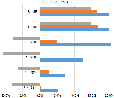
Figure 2: Relative improvement of TransE-NMM against TransE for entity prediction task in WN11 when the filtering threshold $\tau=\{10,100,500\}$ (with other hyper-parameters being the same as selected in Section 4.3). Prefixes “R-” and “F-” denote the “Raw” and “Filtered” settings, respectively. Suffixes “-MR”, “-MRR” and “-H@10” abbreviate the mean rank, the mean reciprocal rank and Hits@10, respectively.

As presented in Table 3, for entity prediction using WN11, TransE-NMM with the filtering threshold $\tau=10$ only obtains better mean rank than TransE (about 15% relative improvement) but lower Hits@10 and mean reciprocal rank. The reason might be that in semantic lexical KBs such as WordNet where relationships between words or word groups are manually constructed, whole neighborhood information might be useful. So when using a small filtering threshold, the model ignores a lot of potential information that could help predicting relationships. Figure 2 presents relative improvements in entity prediction of TransE-NMM over TransE on WN11 when varying the filtering threshold $\tau$. Figure 2 shows that TransE-NMM gains better scores with higher $\tau$ value. Specifically, when $\tau=500$ TransE-NMM does significantly better than TransE in all entity prediction metrics.

6 Conclusion and future work

We introduced a neighborhood mixture model for knowledge base completion by constructing neighbor-based vector representations for entities. We demonstrated its effect by extending TransE [Bordes et al., 2013] with our neighborhood mixture model. On three different datasets, experimental results show that our model significantly improves TransE and obtains better results than the other state-of-the-art embedding models on triple classification, entity prediction and relation prediction tasks. In future work, we plan to apply the neighborhood mixture model to other embedding models, especially to relation path models such as TransE-comp, to combine the useful information from both relation paths and entity neighborhoods.

References

- [Bollacker et al., 2008] Kurt Bollacker, Colin Evans, Praveen Paritosh, Tim Sturge, and Jamie Taylor. 2008. Freebase: A Collaboratively Created Graph Database for Structuring Human Knowledge. In Proceedings of the 2008 ACM SIGMOD International Conference on Management of Data, pages 1247–1250.
- [Bordes et al., 2011] Antoine Bordes, Jason Weston, Ronan Collobert, and Yoshua Bengio. 2011. Learning Structured Embeddings of Knowledge Bases. In Proceedings of the Twenty-Fifth AAAI Conference on Artificial Intelligence, pages 301–306.
- [Bordes et al., 2012] Antoine Bordes, Xavier Glorot, Jason Weston, and Yoshua Bengio. 2012. A Semantic Matching Energy Function for Learning with Multi-relational Data. Machine Learning, 94(2):233–259.
- [Bordes et al., 2013] Antoine Bordes, Nicolas Usunier, Alberto Garcia-Duran, Jason Weston, and Oksana Yakhnenko. 2013. Translating Embeddings for Modeling Multi-relational Data. In Advances in Neural Information Processing Systems 26, pages 2787–2795.
- [Carlson et al., 2010] Andrew Carlson, Justin Betteridge, Bryan Kisiel, Burr Settles, Estevam R. Hruschka, Jr., and Tom M. Mitchell. 2010. Toward an Architecture for Never-ending Language Learning. In Proceedings of the Twenty-Fourth AAAI Conference on Artificial Intelligence, pages 1306–1313.
- [Das et al., 2017] Rajarshi Das, Arvind Neelakantan, David Belanger, and Andrew McCallum. 2017. Chains of reasoning over entities, relations, and text using recurrent neural networks. In Proceedings of the 15th Conference of the European Chapter of the Association for Computational Linguistics.
- [Duchi et al., 2011] John Duchi, Elad Hazan, and Yoram Singer. 2011. Adaptive Subgradient Methods for Online Learning and Stochastic Optimization. The Journal of Machine Learning Research, 12:2121–2159.
- [Feng et al., 2016a] Jun Feng, Minlie Huang, Mingdong Wang, Mantong Zhou, Yu Hao, and Xiaoyan Zhu. 2016a. Knowledge graph embedding by flexible translation. In Principles of Knowledge Representation and Reasoning: Proceedings of the Fifteenth International Conference, pages 557–560.
- [Feng et al., 2016b] Jun Feng, Minlie Huang, Yang Yang, and xiaoyan zhu. 2016b. GAKE: Graph Aware Knowledge Embedding. In Proceedings of COLING 2016, the 26th International Conference on Computational Linguistics: Technical Papers, pages 641–651.
- [García-Durán et al., 2015] Alberto García-Durán, Antoine Bordes, and Nicolas Usunier. 2015. Composing Relationships with Translations. In Proceedings of the 2015 Conference on Empirical Methods in Natural Language Processing, pages 286–290.
- [García-Durán et al., 2016] Alberto García-Durán, Antoine Bordes, Nicolas Usunier, and Yves Grandvalet. 2016. Combining Two and Three-Way Embedding Models for Link Prediction in Knowledge Bases. Journal of Artificial Intelligence Research, 55:715–742.
- [Guo et al., 2015] Shu Guo, Quan Wang, Bin Wang, Lihong Wang, and Li Guo. 2015. Semantically Smooth Knowledge Graph Embedding. In Proceedings of the 53rd Annual Meeting of the Association for Computational Linguistics and the 7th International Joint Conference on Natural Language Processing (Volume 1: Long Papers), pages 84–94.
- [Guu et al., 2015] Kelvin Guu, John Miller, and Percy Liang. 2015. Traversing Knowledge Graphs in Vector Space. In Proceedings of the 2015 Conference on Empirical Methods in Natural Language Processing, pages 318–327.
- [He et al., 2015] Shizhu He, Kang Liu, Guoliang Ji, and Jun Zhao. 2015. Learning to Represent Knowledge Graphs with Gaussian Embedding. In Proceedings of the 24th ACM International on Conference on Information and Knowledge Management, pages 623–632.
- [Jenatton et al., 2012] Rodolphe Jenatton, Nicolas L. Roux, Antoine Bordes, and Guillaume R Obozinski. 2012. A latent factor model for highly multi-relational data. In Advances in Neural Information Processing Systems 25, pages 3167–3175.
- [Ji et al., 2015] Guoliang Ji, Shizhu He, Liheng Xu, Kang Liu, and Jun Zhao. 2015. Knowledge Graph Embedding via Dynamic Mapping Matrix. In Proceedings of the 53rd Annual Meeting of the Association for Computational Linguistics and the 7th International Joint Conference on Natural Language Processing (Volume 1: Long Papers), pages 687–696.
- [Ji et al., 2016] Guoliang Ji, Kang Liu, Shizhu He, and Jun Zhao. 2016. Knowledge Graph Completion with Adaptive Sparse Transfer Matrix. In Proceedings of the Thirtieth AAAI Conference on Artificial Intelligence, pages 985–991.
- [Krompaß et al., 2015] Denis Krompaß, Stephan Baier, and Volker Tresp. 2015. Type-Constrained Representation Learning in Knowledge Graphs. In Proceedings of the 14th International Semantic Web Conference, pages 640–655.
- [Lehmann et al., 2015] Jens Lehmann, Robert Isele, Max Jakob, Anja Jentzsch, Dimitris Kontokostas, Pablo N. Mendes, Sebastian Hellmann, Mohamed Morsey, Patrick van Kleef, Sören Auer, and Christian Bizer. 2015. DBpedia - A Large-scale, Multilingual Knowledge Base Extracted from Wikipedia. Semantic Web, 6(2):167–195.
- [Liang and Forbus, 2015] Chen Liang and Kenneth D. Forbus. 2015. Learning Plausible Inferences from Semantic Web Knowledge by Combining Analogical Generalization with Structured Logistic Regression. In Proceedings of the Twenty-Ninth AAAI Conference on Artificial Intelligence, pages 551–557.
- [Lin et al., 2015a] Yankai Lin, Zhiyuan Liu, Huanbo Luan, Maosong Sun, Siwei Rao, and Song Liu. 2015a. Modeling Relation Paths for Representation Learning of Knowledge Bases. In Proceedings of the 2015 Conference on Empirical Methods in Natural Language Processing, pages 705–714.
- [Lin et al., 2015b] Yankai Lin, Zhiyuan Liu, Maosong Sun, Yang Liu, and Xuan Zhu. 2015b. Learning Entity and Relation Embeddings for Knowledge Graph Completion. In Proceedings of the Twenty-Ninth AAAI Conference on Artificial Intelligence Learning, pages 2181–2187.
- [Liu and Nocedal, 1989] D. C. Liu and J. Nocedal. 1989. On the Limited Memory BFGS Method for Large Scale Optimization. Mathematical Programming, 45(3):503–528.
- [Liu et al., 2016] Qiao Liu, Liuyi Jiang, Minghao Han, Yao Liu, and Zhiguang Qin. 2016. Hierarchical Random Walk Inference in Knowledge Graphs. In Proceedings of the 39th International ACM SIGIR Conference on Research and Development in Information Retrieval, pages 445–454.
- [Luo et al., 2015] Yuanfei Luo, Quan Wang, Bin Wang, and Li Guo. 2015. Context-Dependent Knowledge Graph Embedding. In Proceedings of the 2015 Conference on Empirical Methods in Natural Language Processing, pages 1656–1661.
- [Mikolov et al., 2013] Tomas Mikolov, Wen-tau Yih, and Geoffrey Zweig. 2013. Linguistic Regularities in Continuous Space Word Representations. In Proceedings of the 2013 Conference of the North American Chapter of the Association for Computational Linguistics: Human Language Technologies, pages 746–751.
- [Miller, 1995] George A. Miller. 1995. WordNet: A Lexical Database for English. Communications of the ACM, 38(11):39–41.
- [Neelakantan et al., 2015] Arvind Neelakantan, Benjamin Roth, and Andrew McCallum. 2015. Compositional Vector Space Models for Knowledge Base Completion. In Proceedings of the 53rd Annual Meeting of the Association for Computational Linguistics and the 7th International Joint Conference on Natural Language Processing (Volume 1: Long Papers), pages 156–166.
- [Nguyen et al., 2016] Dat Quoc Nguyen, Kairit Sirts, Lizhen Qu, and Mark Johnson. 2016. STransE: a novel embedding model of entities and relationships in knowledge bases. In Proceedings of the 2016 Conference of the North American Chapter of the Association for Computational Linguistics: Human Language Technologies, pages 460–466.
- [Nickel et al., 2011] Maximilian Nickel, Volker Tresp, and Hans-Peter Kriegel. 2011. A Three-Way Model for Collective Learning on Multi-Relational Data. In Proceedings of the 28th International Conference on Machine Learning, pages 809–816.
- [Nickel et al., 2016a] Maximilian Nickel, Kevin Murphy, Volker Tresp, and Evgeniy Gabrilovich. 2016a. A Review of Relational Machine Learning for Knowledge Graphs. Proceedings of the IEEE, 104(1):11–33.
- [Nickel et al., 2016b] Maximilian Nickel, Lorenzo Rosasco, and Tomaso Poggio. 2016b. Holographic embeddings of knowledge graphs. In Proceedings of the Thirtieth AAAI Conference on Artificial Intelligence, pages 1955–1961.
- [Niepert, 2016] Mathias Niepert. 2016. Discriminative Gaifman Models. In Advances in Neural Information Processing Systems 29, pages 3405–3413.
- [Pennington et al., 2014] Jeffrey Pennington, Richard Socher, and Christopher Manning. 2014. Glove: Global Vectors for Word Representation. In Proceedings of the 2014 Conference on Empirical Methods in Natural Language Processing, pages 1532–1543.
- [Shi and Weninger, 2017] Baoxu Shi and Tim Weninger. 2017. ProjE: Embedding Projection for Knowledge Graph Completion. In Proceedings of the 31st AAAI Conference on Artificial Intelligence.
- [Socher et al., 2013] Richard Socher, Danqi Chen, Christopher D Manning, and Andrew Ng. 2013. Reasoning With Neural Tensor Networks for Knowledge Base Completion. In Advances in Neural Information Processing Systems 26, pages 926–934.
- [Suchanek et al., 2007] Fabian M. Suchanek, Gjergji Kasneci, and Gerhard Weikum. 2007. YAGO: A Core of Semantic Knowledge. In Proceedings of the 16th International Conference on World Wide Web, pages 697–706.
- [Taskar et al., 2004] Ben Taskar, Ming fai Wong, Pieter Abbeel, and Daphne Koller. 2004. Link Prediction in Relational Data. In Advances in Neural Information Processing Systems 16, pages 659–666.
- [Tay et al., 2017] Yi Tay, Anh Tuan Luu, Siu Cheung Hui, and Falk Brauer. 2017. Random Semantic Tensor Ensemble for Scalable Knowledge Graph Link Prediction. In Proceedings of the Tenth ACM International Conference on Web Search and Data Mining, pages 751–760.
- [Toutanova et al., 2016] Kristina Toutanova, Victoria Lin, Wen-tau Yih, Hoifung Poon, and Chris Quirk. 2016. Compositional Learning of Embeddings for Relation Paths in Knowledge Base and Text. In Proceedings of the 54th Annual Meeting of the Association for Computational Linguistics (Volume 1: Long Papers), pages 1434–1444.
- [Trouillon et al., 2016] Théo Trouillon, Johannes Welbl, Sebastian Riedel, Éric Gaussier, and Guillaume Bouchard. 2016. Complex Embeddings for Simple Link Prediction. In Proceedings of the 33nd International Conference on Machine Learning, pages 2071–2080.
- [Wang and Li, 2016] Zhigang Wang and Juan-Zi Li. 2016. Text-Enhanced Representation Learning for Knowledge Graph. In Proceedings of the Twenty-Fifth International Joint Conference on Artificial Intelligence, pages 1293–1299.
- [Wang et al., 2014] Zhen Wang, Jianwen Zhang, Jianlin Feng, and Zheng Chen. 2014. Knowledge Graph Embedding by Translating on Hyperplanes. In Proceedings of the Twenty-Eighth AAAI Conference on Artificial Intelligence, pages 1112–1119.
- [Wang et al., 2016] Quan Wang, Jing Liu, Yuanfei Luo, Bin Wang, and Chin-Yew Lin. 2016. Knowledge Base Completion via Coupled Path Ranking. In Proceedings of the 54th Annual Meeting of the Association for Computational Linguistics (Volume 1: Long Papers), pages 1308–1318.
- [Wei et al., 2016] Zhuoyu Wei, Jun Zhao, and Kang Liu. 2016. Mining Inference Formulas by Goal-Directed Random Walks. In Proceedings of the 2016 Conference on Empirical Methods in Natural Language Processing, pages 1379–1388.
- [West et al., 2014] Robert West, Evgeniy Gabrilovich, Kevin Murphy, Shaohua Sun, Rahul Gupta, and Dekang Lin. 2014. Knowledge Base Completion via Search-based Question Answering. In Proceedings of the 23rd International Conference on World Wide Web, pages 515–526.
- [Xiao et al., 2016a] Han Xiao, Minlie Huang, and Xiaoyan Zhu. 2016a. From One Point to a Manifold: Knowledge Graph Embedding for Precise Link Prediction. In Proceedings of the Twenty-Fifth International Joint Conference on Artificial Intelligence, pages 1315–1321.
- [Xiao et al., 2016b] Han Xiao, Minlie Huang, and Xiaoyan Zhu. 2016b. TransG : A Generative Model for Knowledge Graph Embedding. In Proceedings of the 54th Annual Meeting of the Association for Computational Linguistics (Volume 1: Long Papers), pages 2316–2325.
- [Yang et al., 2015] Bishan Yang, Wen-tau Yih, Xiaodong He, Jianfeng Gao, and Li Deng. 2015. Embedding Entities and Relations for Learning and Inference in Knowledge Bases. In Proceedings of the International Conference on Learning Representations.
- [Yoon et al., 2016] Hee-Geun Yoon, Hyun-Je Song, Seong-Bae Park, and Se-Young Park. 2016. A Translation-Based Knowledge Graph Embedding Preserving Logical Property of Relations. In Proceedings of the 2016 Conference of the North American Chapter of the Association for Computational Linguistics: Human Language Technologies, pages 907–916.
- [Zeiler, 2012] Matthew D. Zeiler. 2012. ADADELTA: An Adaptive Learning Rate Method. CoRR, abs/1212.5701.