Hydrodynamic interaction between particles near elastic interfaces

Abstract

We present an analytical calculation of the hydrodynamic interaction between two spherical particles near an elastic interface such as a cell membrane. The theory predicts the frequency dependent self- and pair-mobilities accounting for the finite particle size up to the 5th order in the ratio between particle diameter and wall distance as well as between diameter and interparticle distance. We find that particle motion towards a membrane with pure bending resistance always leads to mutual repulsion similar as in the well-known case of a hard-wall. In the vicinity of a membrane with shearing resistance, however, we observe an attractive interaction in a certain parameter range which is in contrast to the behavior near a hard wall. This attraction might facilitate surface chemical reactions. Furthermore, we show that there exists a frequency range in which the pair-mobility for perpendicular motion exceeds its bulk value, leading to short-lived superdiffusive behavior. Using the analytical particle mobilities we compute collective and relative diffusion coefficients. The appropriateness of the approximations in our analytical results is demonstrated by corresponding boundary integral simulations which are in excellent agreement with the theoretical predictions.

I Introduction

The hydrodynamic interaction between particles moving through a liquid is essential to determine the behavior of colloidal suspensions Morrone, Li, and Berne (2012), polymer solutions Usta, Ladd, and Butler (2005); Wojciechowski, Szymczak, and Cieplak (2010), chemical reaction kinetics von Hansen, Netz, and Hinczewski (2010); Długosz et al. (2012), bilayer assembly Ando and Skolnick (2013) or cellular flows Popel and Johnson (2005); Misbah and Wagner (2013). As an example, hydrodynamic interactions result in a notable alteration of the collective motion behavior of catalytically powered self-propelled particles Molina, Nakayama, and Yamamoto (2013) or bacterial suspensions Wensink et al. (2012); Dunkel et al. (2013); Lopez and Lauga (2014); Zöttl and Stark (2014); Elgeti, Winkler, and Gompper (2015). Many of the occurring phenomena can be explained on the basis of two-particle interactions Guazzelli and Morris (2012) which in bulk are well understood. Some of the most intriguing observations, however, are made when particles interact hydrodynamically in the close vicinity of interfaces – a prominent example being the attraction of like-charged colloid particles during their motion away from a hard wall Larsen, Grier et al. (1997); Squires and Brenner (2000); Behrens and Grier (2001).

In the low Reynolds number regime hydrodynamic interactions between two particles are fully described by the mobility tensor which provides a linear relation between the force applied on one particle and the resulting velocity of either the same or the neighboring particle. In an unbounded flow, algebraic expressions for the hydrodynamic interactions between two Felderhof (1977); Kim and Mifflin (1985); Yoon and Kim (1987); Cichocki, Felderhof, and Schmitz (1988); Happel and Brenner (2012); Guazzelli and Morris (2012) and several Deutch and Oppenheim (1971); Batchelor (1976); Ermak and McCammon (1978); Ladd (1988); Ekiel-Jeżewska and Felderhof (2015); Zia, Swan, and Su (2015) spherical particles are well established. Experimentally, the predicted hydrodynamic coupling has been confirmed using optical tweezers Crocker (1997); Meiners and Quake (1999); Bartlett, Henderson, and Mitchell (2001); Henderson, Mitchell, and Bartlett (2002) and atomic force microscopy Radiom et al. (2015).

The presence of an interface is known to drastically alter the hydrodynamic mobility. For a single particle, this wall-induced drag effect has been studied extensively over recent decades theoretically and numerically near a rigid Lauga and Squires (2005); Lorentz (1907); MacKay and Mason (1961); Gotoh and Kaneda (1982); Cichocki and Jones (1998); Franosch and Jeney (2009); Felderhof (2012); Padding and Briels (2010); De Corato et al. (2015); Huang and Szlufarska (2015), a fluid-fluid Lee, Chadwick, and Leal (1979); Berdan and Leal (1982); Bickel (2006, 2007); Bławzdziewicz, Ekiel-Jeżewska, and Wajnryb (2010a, b) or an elastic interface Felderhof (2006); Shlomovitz et al. (2013, 2014); Salez and Mahadevan (2015); Daddi-Moussa-Ider, Guckenberger, and Gekle (2016a, b); Saintyves et al. (2016). While rigid interfaces in general simply lead to a reduction of particle mobility, the memory effect caused by elastic interfaces leads to a frequency dependence of the particle mobility and can cause novel phenomena such as transient subdiffusion Daddi-Moussa-Ider, Guckenberger, and Gekle (2016a). On the experimental side, the single particle mobility has been investigated using optical tweezers Faucheux and Libchaber (1994); Dufresne, Altman, and Grier (2001); Schäffer, Nørrelykke, and Howard (2007), evanescent wave dynamic light scattering Holmqvist, Dhont, and Lang (2007); Michailidou et al. (2009); Wang, Prabhakar, and Sevick (2009); Kazoe and Yoda (2011); Lisicki et al. (2012); Rogers et al. (2012); Michailidou et al. (2013); Wang and Huang (2014); Watarai and Iwai (2014); Lisicki et al. (2014) or video microscopy Eral et al. (2010); Cervantes-Martínez et al. (2011); Dettmer et al. (2014). The influence of a nearby elastic cell membrane has recently been investigated using magnetic particle actuation Irmscher et al. (2012) and optical traps Shlomovitz et al. (2013); Boatwright et al. (2014); Jünger et al. (2015).

Hydrodynamic interactions between two particles near a planar rigid wall have been studied theoretically Squires and Brenner (2000); Swan and Brady (2007) and experimentally using optical tweezers Lele et al. (2011); Tränkle, Ruh, and Rohrbach (2016) and digital video microscopy Dufresne et al. (2000). Narrow channels Cui, Diamant, and Lin (2002); Misiunas et al. (2015), 2D confinement Bleibel et al. (2014) or liquid-liquid interfaces have also been investigated Zhang et al. (2013, 2014). Near elastic interfaces, however, no work regarding hydrodynamic interactions has so far been reported. Given the complex behavior of a single particle near an elastic interface (caused by the above-mentioned memory effect) such hydrodynamic interactions can be expected to present a very rich phenomenology.

In this paper, we calculate the motion of two spherical particles positioned above an elastic membrane both analytically and numerically. We find that the shearing and bending related parts in the pair-mobility can in some situations have opposite contributions to the total mobility. Most prominently, we find that two particles approaching an idealized membrane exhibiting only shear resistance will be attracted to each other which is just opposite to the well-known hydrodynamic repulsion for motion towards a hard wall Squires and Brenner (2000). Additionally, we show that the pair-mobility at intermediate frequencies may even exceed its bulk value, a feature which is not observed in bulk or near a rigid wall. This increase in pair-mobility results in a short-lived superdiffusion in the joint mean-square displacement.

The remainder of the paper is organized as follows. In Sec. II, we introduce the theoretical approach to computing the frequency-dependent self- and pair-mobilities from the multipole expansion and Faxén’s theorem, up to the 5th order in the ratio between particle radius and particle-wall or particle-particle distance. In Sec. III, we present the boundary integral method which we have used to numerically confirm our theoretical predictions. In Sec. IV, we provide analytical expressions of the particle self- and pair-mobilities in terms of power series, finding excellent agreement with our numerical simulations. Expressions of the self- and pair-diffusion coefficients are derived in Sec. V. Concluding remarks are made in Sec. VI.

II Theory

Figure 1: Illustration of the problem setup. Two small particles labeled $\gamma$ and $\lambda$ of radius $a$ are located a distance $h:=x_{\lambda}-x_{\gamma}$ apart and a distance $z_{0}$ above an elastic membrane. The dimensionless length scales of the problem are $\epsilon:=a/z_{0}$ and $\sigma:=a/h$.

We consider a pair of particles of radius $a$ suspended in a Newtonian fluid of viscosity $\eta$ above a planar elastic membrane extending in the $xy$ plane. The two particles are placed at $\bm{r}_{\gamma}=(x_{\gamma},0,z_{0})$ and $\bm{r}_{\lambda}=(x_{\lambda},0,z_{0})$, i.e. the line connecting the two particles is parallel to the undisplaced membrane. We denote by $h:=x_{\lambda}-x_{\gamma}$ the center-to-center separation measured from the left ($\gamma$) to the right ($\lambda$) particle (see Fig. 1 for an illustration).

The particle mobility is a tensorial quantity that linearly couples the velocity ${V_{\gamma}}_{\alpha}$ of particle $\gamma$ in direction $\alpha$ to an external force in the direction $\beta$ applied on the same (${F_{\gamma}}_{\beta}$) or the other (${F_{\lambda}}_{\beta}$) particle. Transforming to the frequency domain we thus have (Kim and Karrila, 2005, ch. 7)

$${V_{\gamma}}_{\alpha}(\omega)=\mu_{\alpha\beta}^{\gamma\gamma}(\bm{r}_{\gamma},\bm{r}_{\gamma},\omega){F_{\gamma}}_{\beta}(\omega)+\mu_{\alpha\beta}^{\gamma\lambda}(\bm{r}_{\gamma},\bm{r}_{\lambda},\omega){F_{\lambda}}_{\beta}(\omega)\,,$$

where Einstein’s convention for summation over repeated indices is assumed. The particle mobility tensor in the present geometry can be written as an algebraic sum of two distinct contributions

$$\mu_{\alpha\beta}^{\gamma\lambda}(\bm{r}_{\gamma},\bm{r}_{\lambda},\omega)={b}_{\alpha\beta}^{\gamma\lambda}(\bm{r}_{\gamma},\bm{r}_{\lambda})+\Delta\mu_{\alpha\beta}^{\gamma\lambda}(\bm{r}_{\gamma},\bm{r}_{\lambda},\omega)\,,$$ (1)

where ${b}_{\alpha\beta}^{\gamma\lambda}$ is the pair-mobility in an unbounded geometry (bulk flow), and $\Delta\mu_{\alpha\beta}^{\gamma\lambda}$ is the frequency-dependent correction due to the presence of the elastic membrane. An analogous relation holds for $\mu_{\alpha\beta}^{\gamma\gamma}$.

For the determination of the particle mobility, we consider a force density $\bm{f}$ acting on the surface $S_{\lambda}$ of the particle $\lambda$, related to the total force by

$${{F}_{\lambda}}_{\beta}(\omega)=\oint_{S_{\lambda}}{f}_{\beta}(\bm{r}^{\prime},\omega)\mathrm{d}^{2}\bm{r}^{\prime}\,,$$

which induces the disturbance flow velocity at point $\bm{r}$

$$v_{\alpha}(\bm{r},\bm{r}_{\lambda},\omega)=\oint_{S_{\lambda}}\mathcal{G}_{\alpha\beta}(\bm{r},\bm{r}^{\prime},\omega)f_{\beta}(\bm{r}^{\prime},\omega)\mathrm{d}^{2}\bm{r}^{\prime}\,,$$ (2)

where $\mathcal{G}_{\alpha\beta}$ denotes the velocity Green’s function (Stokeslet), i.e. the flow velocity field resulting from a point-force acting on $\bm{r}_{\lambda}$. The disturbance velocity at any point $\bm{r}$ can be split up into two parts,

$$v_{\alpha}(\bm{r},\bm{r}_{\lambda},\omega)={v}_{\alpha}^{(0)}(\bm{r},\bm{r}_{\lambda})+\Delta v_{\alpha}(\bm{r},\bm{r}_{\lambda},\omega)\,,$$ (3)

where ${v}_{\alpha}^{(0)}$ is the flow field induced by the particle $\lambda$ in an unbounded geometry, and $\Delta v_{\alpha}$ is the flow satisfying the no-slip boundary condition at the membrane. In this way, the Green’s function can be written as

$$\mathcal{G}_{\alpha\beta}(\bm{r},\bm{r}^{\prime},\omega)=\mathcal{G}_{\alpha\beta}^{(0)}(\bm{r},\bm{r}^{\prime})+\Delta\mathcal{G}_{\alpha\beta}(\bm{r},\bm{r}^{\prime},\omega)\,,$$ (4)

where $\mathcal{G}_{\alpha\beta}^{(0)}$ is the infinite-space Green’s function (Oseen’s tensor) given by

$$\mathcal{G}_{\alpha\beta}^{(0)}(\bm{r},\bm{r}^{\prime})=\frac{1}{8\pi\eta}\left(\frac{\delta_{\alpha\beta}}{s}+\frac{{s}_{\alpha}{s}_{\beta}}{s^{3}}\right)\,,$$ (5)

with $\bm{s}:=\bm{r}-\bm{r}^{\prime}$ and $s:=|\bm{s}|$. The term $\Delta\mathcal{G}_{\alpha\beta}$ represents the frequency-dependent correction due to the presence of the membrane. Far away from the particle $\lambda$, the vector $\bm{r}^{\prime}$ in Eq. (2) can be expanded around the particle center $\bm{r}_{\lambda}$ following a multipole expansion approach. Up to the second order, and assuming a constant force density, the disturbance velocity can be approximated by Kim and Netz (2006); Gauger, Downton, and Stark (2008); Swan and Brady (2007, 2010)

$$v_{\alpha}(\bm{r},\bm{r}_{\lambda},\omega)\approx\left(1+\frac{a^{2}}{6}\bm{\nabla}_{\bm{r}_{\lambda}}^{2}\right)\mathcal{G}_{\alpha\beta}(\bm{r},\bm{r}_{\lambda},\omega){F_{\lambda}}_{\beta}(\omega)\,,$$ (6)

where $\bm{\nabla}_{\bm{r}_{\lambda}}$ stands for the gradient operator taken with respect to the singularity position $\bm{r}_{\lambda}$. Note that for a single sphere in bulk, the flow field given by Eq. (6) satisfies exactly the no-slip boundary conditions at the surface of the sphere, i.e. in the frame moving with the particle, both the normal and tangential velocities vanish. Using Faxén’s theorem, the velocity of the second particle $\gamma$ in this flow reads Kim and Netz (2006); Gauger, Downton, and Stark (2008); Swan and Brady (2007, 2010)

$${V_{\gamma}}_{\alpha}(\omega)=\mu_{0}{{F}_{\gamma}}_{\alpha}(\omega)+\left(1+\frac{a^{2}}{6}\bm{\nabla}_{\bm{r}_{\gamma}}^{2}\right)v_{\alpha}(\bm{r}_{\gamma},\bm{r}_{\lambda},\omega)\,,$$ (7)

where $\mu_{0}:=1/(6\pi\eta a)$ denotes the usual bulk mobility, given by the Stokes’ law. The disturbance flow $v_{\alpha}$ incorporates both the disturbance from the particle $\lambda$ and the disturbance caused by the presence of the membrane. By plugging Eq. (6) into Faxén’s formula given by Eq. (7), the $\alpha\beta$ component of the frequency-dependent pair-mobilities can be obtained from

$$\mu_{\alpha\beta}^{\gamma\lambda}(\omega)=\left(1+\frac{a^{2}}{6}\bm{\nabla}_{\bm{r}_{\gamma}}^{2}\right)\left(1+\frac{a^{2}}{6}\bm{\nabla}_{\bm{r}_{\lambda}}^{2}\right)\mathcal{G}_{\alpha\beta}(\bm{r}_{\gamma},\bm{r}_{\lambda},\omega)\,.$$ (8)

For the self-mobilities, only the correction in the flow field $\Delta v_{\alpha}$ due to the presence of the membrane in Eq. (3) is considered in Faxén’s formula (the influence of the second particle on the self-mobility is neglected here for simplicity Swan and Brady (2007); Gauger, Downton, and Stark (2008)). Therefore, the frequency-dependent self-mobilities read

$$\begin{split}\mu_{\alpha\beta}^{\gamma\gamma}(\omega)&=\mu_{0}+\lim_{\bm{r}\to\bm{r}_{\gamma}}\left(1+\frac{a^{2}}{6}\bm{\nabla}_{\bm{r}}^{2}\right)\\ &\quad\times\left(1+\frac{a^{2}}{6}\bm{\nabla}_{\bm{r}_{\gamma}}^{2}\right)\Delta\mathcal{G}_{\alpha\beta}(\bm{r},\bm{r}_{\gamma},\omega)\,\end{split}$$ (9)

and analogously for $\mu_{\alpha\beta}^{\lambda\lambda}$.

In order to use the particle pair- and self-mobilities from Eqs. (8) and (9), the velocity Green’s functions in the presence of the membrane are required. These have been calculated in our earlier work Daddi-Moussa-Ider, Guckenberger, and Gekle (2016a) and their derivation is only briefly sketched here with more details in Appendix A.

We proceed by solving the steady Stokes equations with an arbitrary time-dependent point-force $\bm{F}$ acting at $\bm{r}_{0}=(0,0,z_{0})$,

$$\eta\bm{\nabla}^{2}\bm{v}-\bm{\nabla}p+\bm{F}\delta(\bm{r}-\bm{r}_{0}) =0\,,$$ (10)

$$\bm{\nabla}\cdot\bm{v} =0\,,$$ (11)

where $p$ is the pressure field. The determination of the Green’s functions at $\bm{r}_{\lambda}$ is straightforward thanks to the system translational symmetry along the $xy$ plane. After solving the above equations and appropriately applying the boundary conditions at the membrane, we find that the Green’s functions are conveniently expressed by

$${\mathcal{G}}_{zz}(\bm{r},\bm{r}_{\lambda},\omega) =\frac{1}{2\pi}\int_{0}^{\infty}\tilde{\mathcal{G}}_{zz}(q,z,z_{0},\omega)J_{0}(\rho q)q\mathrm{d}q\,,$$ (12a)

$$\mathcal{G}_{xx}(\bm{r},\bm{r}_{\lambda},\omega) =\frac{1}{4\pi}\int_{0}^{\infty}\bigg{(}\tilde{\mathcal{G}}_{+}(q,z,z_{0},\omega)J_{0}(\rho q)$$

$$+\tilde{\mathcal{G}}_{-}(q,z,z_{0},\omega)J_{2}(\rho q)\cos 2\theta\bigg{)}q\mathrm{d}q\,,$$ (12b)

$$\mathcal{G}_{yy}(\bm{r},\bm{r}_{\lambda},\omega) =\frac{1}{4\pi}\int_{0}^{\infty}\bigg{(}\tilde{\mathcal{G}}_{+}(q,z,z_{0},\omega)J_{0}(\rho q)$$

$$-\tilde{\mathcal{G}}_{-}(q,z,z_{0},\omega)J_{2}(\rho q)\cos 2\theta\bigg{)}q\mathrm{d}q\,,$$ (12c)

$$\mathcal{G}_{xz}(\bm{r},\bm{r}_{\lambda},\omega) =\frac{i\cos\theta}{2\pi}\int_{0}^{\infty}\tilde{\mathcal{G}}_{lz}(q,z,z_{0},\omega)J_{1}(\rho q)\mathrm{d}q\,,$$ (12d)

where $\rho:=\sqrt{(x-x_{\lambda})^{2}+y^{2}}$, $\theta:=\arctan(y/(x-x_{\lambda}))$ with $\bm{r}=(x,y,z)$. Here $J_{n}$ denotes the Bessel function of the first kind of order $n$. The functions $\tilde{\mathcal{G}}_{\pm}$, $\tilde{\mathcal{G}}_{lz}$ and $\tilde{\mathcal{G}}_{zz}$ are provided in Appendix A. It is worth to mention here that the unsteady term in the Stokes equations leads to negligible contribution in the correction to the Green’s functions Daddi-Moussa-Ider, Guckenberger, and Gekle (2016a), and it is therefore not considered in the present work.

The membrane elasticity is described by the well-established Skalak model Skalak et al. (1973), commonly used to describe deformation properties of red blood cell (RBC) membranes Eggleton and Popel (1998); Krüger, Varnik, and Raabe (2011); Krüger (2012). The elastic model has as parameters the shearing modulus $\kappa_{\mathrm{S}}$ and the area-expansion modulus $\kappa_{\mathrm{A}}$. The two moduli are related via the dimensionless number $C:=\kappa_{\mathrm{A}}/\kappa_{\mathrm{S}}$. Moreover, the membrane resists towards bending according to Helfrich’s model Helfrich (1973), with the corresponding bending rigidity $\kappa_{\mathrm{B}}$.

III Boundary integral methods

In this section, we introduce the numerical method used to compute the particle self- and pair- mobilities. The numerical results will subsequently be compared with the analytical predictions presented in Sec. II.

For solving the fluid motion equations in the inertia-free Stokes regime, we use a boundary integral method (BIM). The method is well suited for problems with deforming boundaries such as RBC membranes Pozrikidis (2001); Zhao and Shaqfeh (2011). In order to solve for the particle velocity given an exerted force, a completed double layer boundary integral method (CDLBIM) Power and Miranda (1987); Kohr and Pop (2004) has been combined with the classical BIM Zhao, Shaqfeh, and Narsimhan (2012). The integral equations for the two-particle membrane systems read

$$\begin{split}v_{\beta}(\bm{x})&=H_{\beta}(\bm{x})\,,\quad\bm{x}\in S_{\mathrm{m}}\,,\\ \frac{1}{2}\phi_{\beta}(\bm{x})+\sum_{\alpha=1}^{6}\varphi_{\beta}^{(\alpha)}(\bm{x})\braket{\bm{\varphi}^{(\alpha)},\bm{\phi}}&=H_{\beta}(\bm{x})\,,\quad\bm{x}\in S_{\mathrm{p}}\,.\end{split}$$ (13)

where $S_{\mathrm{m}}$ is the surface of the elastic membrane and $S_{\mathrm{p}}:=S_{\mathrm{p}_{\gamma}}\cup S_{\mathrm{p}_{\lambda}}$ is the surface of the two spheres. Here $\bm{v}$ denotes the velocity on the membrane whereas $\bm{\phi}$ represents the double layer density function on $S_{\mathrm{p}}$, related to the velocity of the particle $\gamma$ via

$${V_{\gamma}}_{\beta}(\bm{x})=\sum_{\alpha=1}^{6}\varphi_{\beta}^{(\alpha)}(\bm{x})\braket{\bm{\varphi}^{(\alpha)},\bm{\phi}}\,,\quad\bm{x}\in S_{\mathrm{p}_{\gamma}}\,.$$ (14)

where $\bm{\varphi}^{(\alpha)}$ are known functions Kohr and Pop (2004). The brackets stand for the inner product in the space of real functions whose domain is $S_{\mathrm{p}_{\gamma}}$, and the function $H_{\beta}$ is defined by

$$H_{\beta}(\bm{x}):=-(N_{\mathrm{m}}\Delta\bm{f})_{\beta}(\bm{x})-(K_{\mathrm{p}}\bm{\phi})_{\beta}(\bm{x})+\mathcal{G}_{\beta\mu}^{(0)}(\bm{x},\bm{x}_{\lambda_{\mathrm{c}}})F_{\mu}\,,$$

with $\bm{x}_{\lambda_{\mathrm{c}}}$ being the centroid of the sphere labeled $\lambda$ upon which the force is applied. The single layer integral is defined as

$$(N_{\mathrm{m}}\Delta\bm{f})_{\beta}(\bm{x}):=\int_{S_{\mathrm{m}}}\Delta f_{\alpha}(\bm{y})\mathcal{G}_{\alpha\beta}^{(0)}(\bm{y},\bm{x})\,\mathrm{d}S(\bm{y})$$

and the double layer integral as

$$(K_{\mathrm{p}}\bm{\phi})_{\beta}(\bm{x}):=\oint_{S_{\mathrm{p}}}\phi_{\alpha}(\bm{y})\mathcal{T}_{\alpha\beta\mu}^{(0)}(\bm{y},\bm{x})n_{\mu}(\bm{y})\,\mathrm{d}S(\bm{y})\,.$$

Here, $\Delta\bm{f}$ is the traction jump, $\bm{n}$ denotes the outer normal vector at the particle surfaces and $\bm{F}$ is the force acting on the rigid particle. The infinite-space Green’s function is given by Eq. (5) and the corresponding Stresslet, defined as the symmetric part of the first moment of the force density, reads Kim and Karrila (2005)

$$\mathcal{T}_{\alpha\beta\mu}^{(0)}(\bm{y},\bm{x})=-\frac{3}{4\pi}\frac{s_{\alpha}s_{\beta}s_{\mu}}{s^{5}}\,,$$

with $\bm{s}:=\bm{y}-\bm{x}$ and $s:=|\bm{s}|$. The traction jump across the membrane $\Delta\bm{f}$ is an input for the equations, determined from the instantaneous deformation of the membrane. In order to solve Eqs. (13) numerically, the membrane and particles’ surfaces are discretized with flat triangles. The resulting linear system of equations for the velocity $\bm{v}$ on the membrane and the density $\bm{\phi}$ on the rigid particles is solved iteratively by GMRES Saad and Schultz (1986). The velocity of each particle is determined from (14). For further details concerning the algorithm and its implementation, we refer the reader to Ref. Daddi-Moussa-Ider, Guckenberger, and Gekle (2016a). Bending forces are computed using Method C from Guckenberger et al. (2016).

In order to compute the particle self- and pair-mobilities numerically, a harmonic oscillating force $\bm{F}_{\lambda}(t)=\bm{A}_{\lambda}e^{i\omega_{0}t}$ of amplitude $\bm{A}_{\lambda}$ and frequency $\omega_{0}$ is applied at the surface of the particle $\lambda$. After a brief transient time, both particles begin to oscillate at the same frequency as $\bm{V}_{\lambda}(t)=\bm{B}_{\lambda}e^{i(\omega_{0}t+\delta_{\lambda})}$ and as $\bm{V}_{\gamma}(t)=\bm{B}_{\gamma}e^{i(\omega_{0}t+\delta_{\gamma})}$. The velocity amplitudes and phase shifts can accurately be obtained by a fitting procedure of the numerically recorded particle velocities. For that, we use a nonlinear least-squares algorithm based on the trust region method Conn, Gould, and Toint (2000). Afterward, the $\alpha\beta$ component of the frequency-dependent complex self- and pair-mobilities can be calculated as

$$\mu_{\alpha\beta}^{\lambda\lambda}=\frac{{B_{\lambda}}_{\alpha}}{{A_{\lambda}}_{\beta}}e^{i\delta_{\lambda}}\,,\quad\mu_{\alpha\beta}^{\gamma\lambda}=\frac{{B_{\gamma}}_{\alpha}}{{A_{\lambda}}_{\beta}}e^{i\delta_{\gamma}}\,.$$

IV Results

For a single membrane, the corrections to the particle mobility can conveniently be split up into a correction due to shearing and area expansion together with a correction due to bending Daddi-Moussa-Ider, Guckenberger, and Gekle (2016a). In the following, we denote by $\mu^{\gamma\gamma}_{\alpha\beta}=\mu^{\lambda\lambda}_{\alpha\beta}=\mu^{\mathrm{S}}_{\alpha\beta}$ (“self”) the components of the self-mobility tensor, and by $\mu^{\gamma\lambda}_{\alpha\beta}=\mu^{\lambda\gamma}_{\beta\alpha}=\mu^{\mathrm{P}}_{\alpha\beta}$ (“pair”) the components of the pair-mobility tensor. Note that for $\alpha\neq\beta$, $\mu^{\mathrm{S}}_{\alpha\beta}=0$ and that $\mu^{\mathrm{P}}_{\alpha\beta}=-\mu^{\mathrm{P}}_{\beta\alpha}$.

IV.1 Self-mobilities for finite-sized particles

Mathematical expressions for the translational particle self-mobility corrections will be derived in terms of $\epsilon=a/z_{0}$. The point-particle approximation presented in earlier work Daddi-Moussa-Ider, Guckenberger, and Gekle (2016a) represents the first order in the perturbation series, valid when the particle is far away from the membrane.

IV.1.1 Perpendicular to membrane

The particle mobility perpendicular to the membrane is readily obtained after plugging the correction $\Delta\mathcal{G}_{zz}$ as defined by Eq. (4) to the normal-normal component of the Green’s function from Eq. (12a) into Eq. (9). After computation, we find that the contribution due to shearing and bending can be expressed as

$$\frac{\Delta\mu_{zz,\mathrm{S}}^{\mathrm{S}}}{\mu_{0}} =e^{i\beta}\bigg{(}-\frac{9}{16}\operatorname{E}_{4}(i\beta)\epsilon+\frac{3}{4}\operatorname{E}_{5}(i\beta)\epsilon^{3}$$

$$-\frac{5}{16}\operatorname{E}_{6}(i\beta)\epsilon^{5}\bigg{)}\,,$$ (15a)

$$\frac{\Delta\mu_{zz,\mathrm{B}}^{\mathrm{S}}}{\mu_{0}} =\epsilon f_{1}+\epsilon^{3}f_{3}+\epsilon^{5}f_{5}\,,$$ (15b)

where the subscripts S and B stand for shearing and bending, respectively. The function $\operatorname{E}_{n}$ is the generalized exponential integral defined as $\operatorname{E}_{n}(x):=\int_{1}^{\infty}t^{-n}e^{-xt}\mathrm{d}t$ Abramowitz, Stegun et al. (1972). Furthermore, $\beta:=6Bz_{0}\eta\omega/\kappa_{\mathrm{S}}$ is a dimensionless frequency associated with the shearing resistance, whereas $B:=2/(1+C)$. Moreover, $\beta_{\mathrm{B}}:=2z_{0}(4\eta\omega/\kappa_{\mathrm{B}})^{1/3}$ is a dimensionless number associated with bending. The functions $f_{i}$, with $i\in\{1,3,5\}$ are defined by

$$f_{1} =-\frac{15}{16}+\frac{3i\beta_{\mathrm{B}}}{8}\Bigg{(}\left(\frac{\beta_{\mathrm{B}}^{2}}{12}+\frac{i\beta_{\mathrm{B}}}{6}+\frac{1}{6}\right)\phi_{+}$$

$$+\frac{\sqrt{3}}{6}(\beta_{\mathrm{B}}+i)\phi_{-}+\left(\frac{\beta_{\mathrm{B}}^{2}}{12}-\frac{i\beta_{\mathrm{B}}}{3}-\frac{1}{3}\right)\psi\Bigg{)}\,,$$

$$f_{3} =\frac{5}{16}-\frac{\beta_{\mathrm{B}}^{3}}{48}\bigg{(}\left(\frac{\beta_{\mathrm{B}}}{4}+i\right)\phi_{+}+\frac{i\sqrt{3}\beta_{\mathrm{B}}}{4}\phi_{-}$$

$$-\left(\frac{\beta_{\mathrm{B}}}{2}-i\right)\psi+\frac{3i}{2}\bigg{)}\,,$$

$$f_{5} =-\frac{1}{16}+\frac{\beta_{\mathrm{B}}^{3}}{384}\left(\frac{\beta_{\mathrm{B}}^{2}}{3}\left(\frac{\sqrt{3}}{2}\phi_{-}+\frac{i}{2}\phi_{+}-i\psi\right)+i\right)\,,$$

with

$$\phi_{\pm} :=e^{-i\overline{z_{\mathrm{B}}}}\operatorname{E}_{1}\left(-i\overline{z_{\mathrm{B}}}\right)\pm e^{-iz_{\mathrm{B}}}\operatorname{E}_{1}\left(-iz_{\mathrm{B}}\right)\,,$$

$$\psi :=e^{-i\beta_{\mathrm{B}}}\operatorname{E}_{1}(-i\beta_{\mathrm{B}})\,,$$

where $z_{\mathrm{B}}:=j\beta_{\mathrm{B}}$ and $j:=e^{2i\pi/3}$ being the principal cubic-root of unity. The bar designates complex conjugate.

The total mobility correction is obtained by adding the individual contributions due to shearing and bending, as given by Eqs. (15a) and (15b). In the vanishing frequency limit, the known result for a hard-wall Swan and Brady (2010) is obtained:

$$\lim_{\beta,\beta_{\mathrm{B}}\to 0}\frac{\Delta\mu_{zz}^{\mathrm{S}}}{\mu_{0}}=-\frac{9}{8}\epsilon+\frac{1}{2}\epsilon^{3}-\frac{1}{8}\epsilon^{5}\,.$$ (16)

The particle mobility near an elastic membrane is determined by membrane shearing and bending properties. We therefore consider a typical case for which both effect manifests themselves equally. For that purpose, we define a characteristic time scale for shearing as $T_{\mathrm{S}}:=6z_{0}\eta/\kappa_{\mathrm{S}}$ together with a characteristic time scale for bending as $T_{\mathrm{B}}:=4\eta z_{0}^{3}/\kappa_{\mathrm{B}}$ Daddi-Moussa-Ider, Guckenberger, and Gekle (2016a). Then we take $z_{0}^{2}\kappa_{\mathrm{S}}/\kappa_{\mathrm{B}}=3/2$ such that the two time scales are equal and can be denoted by $T_{\mathrm{S}}=T_{\mathrm{B}}=:T$. In this case, the two dimensionless numbers $\beta$ and $\beta_{\mathrm{B}}$ are related by $\beta_{\mathrm{B}}=2(\beta/B)^{1/3}$. The situation for a membrane with the typical parameters of a red blood cell is qualitatively similar as shown in the Supporting Information.

In Fig. 2 $a)$, we show the particle scaled self-mobility corrections versus the scaled frequency $\beta$, as stated by Eqs. (15a) and (15b). The particle is set a distance $z_{0}=2a$ above the membrane. We observe that the real part is a monotonically increasing function with respect to frequency while the imaginary part exhibits a bell-shaped dependence on frequency centered around $\beta\sim 1$. In the limit of infinite frequencies, both the real and imaginary parts of the self-mobility corrections vanish, and thus one recovers the bulk behavior. For the perpendicular motion we observe that the particle mobility correction is primarily determined by the bending part.

A very good agreement is obtained between the analytical predictions and the numerical simulations over the whole range of frequencies. Additionally, we assess the accuracy of the point-particle approximation employed in earlier work Daddi-Moussa-Ider, Guckenberger, and Gekle (2016a), in which only the first order correction term in the perturbation parameter $\epsilon$ was considered. While this approximation slightly underestimates particle mobilities, it nevertheless leads to a surprisingly good prediction, even though the particle is set only one diameter above the membrane.

IV.1.2 Parallel to membrane

We proceed in a similar way for the motion parallel to the membrane. By plugging the correction $\Delta\mathcal{G}_{xx}$ from the Green’s function in Eq. (12b) into Eq. (9) we find

$$\frac{\Delta\mu_{xx,\mathrm{S}}^{\mathrm{S}}}{\mu_{0}} =e^{i\beta}\bigg{(}-\frac{3}{32}\bigg{(}3\operatorname{E}_{4}(i\beta)-4\operatorname{E}_{3}(i\beta)+2\operatorname{E}_{2}(i\beta)$$

$$+4e^{iC\beta}\operatorname{E}_{2}(i(1+C)\beta)\bigg{)}\epsilon$$ (17a)

$$+\frac{3}{16}\left(2\operatorname{E}_{5}(i\beta)-\operatorname{E}_{4}(i\beta)\right)\epsilon^{3}-\frac{5}{32}\operatorname{E}_{6}(i\beta)\epsilon^{5}\bigg{)}\,,$$

$$\frac{\Delta\mu_{xx,\mathrm{B}}^{\mathrm{S}}}{\mu_{0}} =\epsilon g_{1}+\epsilon^{3}g_{3}+\epsilon^{5}g_{5}\,,$$ (17b)

where we defined

$$g_{1} =-\frac{3}{32}+\frac{i\beta_{\mathrm{B}}^{3}}{64}(\phi_{+}+\psi)\,,$$

$$g_{3} =\frac{3}{32}+\frac{\beta_{\mathrm{B}}^{3}}{64}\left(-i+\frac{\beta_{\mathrm{B}}}{3}\left(\psi-\frac{1}{2}\phi_{+}-\frac{i\sqrt{3}}{2}\phi_{-}\right)\right)\,,$$

$$g_{5} =-\frac{1}{32}+\frac{\beta_{\mathrm{B}}^{3}}{768}\left(i+\frac{\beta_{\mathrm{B}}^{2}}{3}\left(\frac{i}{2}\phi_{+}+\frac{\sqrt{3}}{2}\phi_{-}-i\psi\right)\right)\ .$$

The well-known hard-wall limit, as first calculated by FaxénFaxén (1922); Swan and Brady (2010), is recovered by considering the vanishing frequency limit:

$$\lim_{\beta,\beta_{\mathrm{B}}\to 0}\frac{\Delta\mu_{xx}^{\mathrm{S}}}{\mu_{0}}=-\frac{9}{16}\epsilon+\frac{1}{8}\epsilon^{3}-\frac{1}{16}\epsilon^{5}\,.$$ (18)

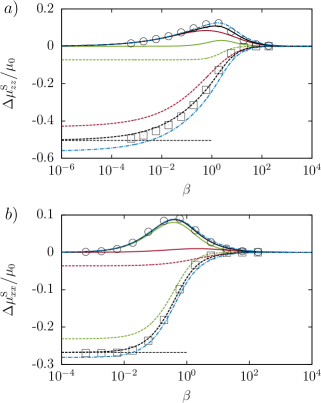
Figure 2: (Color online) The scaled frequency-dependent self-mobility correction versus the scaled frequency for the motion perpendicular $(a)$ and parallel $(b)$ to the membrane. The particle is located at $z_{0}=2a$. We take $z_{0}^{2}\kappa_{\mathrm{S}}/\kappa_{\mathrm{B}}=3/2$ and $C=1$ in the Skalak model. The analytical predictions are shown as dashed lines for the real part, and as solid lines for the imaginary part. Symbols refer to BIM simulations. The shearing and bending contributions are shown in green and red respectively. The dotted-dashed line in blue corresponds to the first order correction in the particle self-mobility, as previously determined in Ref. Daddi-Moussa-Ider, Guckenberger, and Gekle (2016a). Horizontal dashed lines represent the mobility corrections near a hard-wall as given by Eqs. (16) and (18).

The mobility corrections in the parallel direction are shown in Fig. 2 $b)$. We observe that the total correction is mainly determined by the shearing part in contrast to the perpendicular case where bending dominates.

IV.2 Pair-mobilities for finite-sized particles

In the following, expressions for the pair-mobility corrections in terms of a power series in $\sigma=a/h$ will be provided. To start, let us first recall the particle pair-mobilities in an unbounded geometry. By applying Eq. (8) to the infinite space Green’s function Eq. (5), the bulk pair-mobilities for the motion perpendicular to and along the line of centers read (Kim and Karrila, 2005, p. 190)

$$\frac{\mu_{zz}^{\mathrm{P}}}{\mu_{0}}=\frac{3}{4}\sigma+\frac{1}{2}\sigma^{3}\,,\quad\frac{\mu_{xx}^{\mathrm{P}}}{\mu_{0}}=\frac{3}{2}\sigma-\sigma^{3}\,,$$ (19)

and are commonly denominated the Rotne-Prager tensor Rotne and Prager (1969); Ermak and McCammon (1978). Note that the terms with $\sigma^{5}$ vanish for the bulk mobilities when considering only the first reflection as is done here. The axial symmetry along the line connecting the two spheres in bulk requires that $\mu_{yy}^{\mathrm{P}}=\mu_{zz}^{\mathrm{P}}$ and that the off-diagonal components of the mobility tensor are zero. Physically, the parameter $\sigma$ only takes values between 0 and $1/2$ as overlap between the two particles is not allowed. In this interval, the pair-mobility perpendicular to the line of centers $\mu_{zz}^{\mathrm{P}}$ is always lower than the pair-mobility $\mu_{xx}^{\mathrm{P}}$, since it is easier to move the fluid aside than to push it into or to squeeze it out of the gap between the two particles.

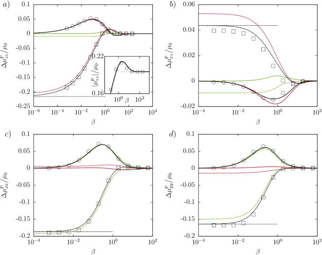
Figure 3: (Color online) The scaled pair-mobility corrections versus the scaled frequency $\beta$. The two particles are located above the membrane at $z_{0}=2a$ with a distance $h=4a$. The real and imaginary parts of the mobility correction are shown as dashed and solid lines, respectively. The shearing and bending related parts are shown in green and red, respectively. The hard-wall limits are shown as horizontal dashed lines. The inset in $a)$ shows that the amplitude of the total pair-mobility component $zz$ exceeds its bulk value (dotted line) in a small frequency range around $\beta\sim 1$.

Consider next the pair-mobilities near an elastic membrane. By applying Eq. (8) to Eqs. (12a) through (12d), we find that the corrections to the pair-mobilities can conveniently be expressed in terms of the following convergent integrals,

$$\frac{\Delta\mu_{zz}^{\mathrm{P}}}{\mu_{0}} =\int_{0}^{\infty}-\frac{i\sigma u^{3}}{3\xi^{5/2}}\left(\frac{\Lambda^{2}}{2iu-\beta}+\frac{4\Gamma_{-}^{2}}{8iu^{3}-\beta_{\mathrm{B}}^{3}}\right)$$

$$\times\chi_{0}e^{-2u}\mathrm{d}u\,,$$ (20a)

$$\frac{\Delta\mu_{xx}^{\mathrm{P}}}{\mu_{0}} =\int_{0}^{\infty}\bigg{(}\frac{i\sigma}{6\xi^{5/2}}\left(\frac{\Gamma_{+}^{2}}{2iu-\beta}+\frac{4u^{4}\Lambda^{2}}{8iu^{3}-\beta_{\mathrm{B}}^{3}}\right)$$

$$\times\left(\xi^{1/2}\chi_{1}-2u\chi_{0}\right)-\frac{3\sigma B}{2}\frac{\chi_{1}}{Bu+i\beta}\bigg{)}e^{-2u}\mathrm{d}u\,,$$ (20b)

$$\frac{\Delta\mu_{yy}^{\mathrm{P}}}{\mu_{0}} =\int_{0}^{\infty}\bigg{(}-\frac{i\sigma}{6\xi^{2}}\left(\frac{\Gamma_{+}^{2}}{2iu-\beta}+\frac{4u^{4}\Lambda^{2}}{8iu^{3}-\beta_{\mathrm{B}}^{3}}\right)\chi_{1}$$

$$+\frac{3\sigma B}{2\xi^{1/2}}\frac{\xi^{1/2}\chi_{1}-2u\chi_{0}}{Bu+i\beta}\bigg{)}e^{-2u}\mathrm{d}u\,,$$ (20c)

$$\frac{\Delta\mu_{xz}^{\mathrm{P}}}{\mu_{0}} =\int_{0}^{\infty}\frac{i\sigma u^{2}}{3\xi^{5/2}}\Lambda\left(\frac{\Gamma_{+}}{2iu-\beta}+\frac{4u^{2}\Gamma_{-}}{8iu^{3}-\beta_{\mathrm{B}}^{3}}\right)$$

$$\times\chi_{1}e^{-2u}\mathrm{d}u\,,$$ (20d)

where $\xi:=4z_{0}^{2}/h^{2}=4\sigma^{2}/\epsilon^{2}$ and

$$\Lambda := 4\sigma^{2}u-3\xi\,,$$

$$\Gamma_{\pm} := 4\sigma^{2}u^{2}-3u\xi\pm 3\xi\,,$$

$$\chi_{n} := J_{n}\left(\frac{2u}{\xi^{1/2}}\right)\,.$$

The terms involving $\beta$ and $\beta_{\mathrm{B}}$ in Eqs. (20a) through (20d) are the contributions coming from shearing and bending, respectively. Due to symmetry, $\mu_{\alpha y}^{\mathrm{P}}=0$ for $\alpha\in\{x,z\}$.

For future reference, we note that each component of the frequency-dependent particle self- and pair-mobility tensor can conveniently be cast in the form

$$\frac{\mu(\omega)}{\mu_{0}}=b+\int_{0}^{\infty}\frac{\varphi_{1}(u)}{\varphi_{2}(u)+i\omega T}\mathrm{d}u\,,$$ (21)

where indices and superscripts have been omitted. Here $b$ denotes the scaled bulk mobility (cf. Eq. (1)), and the integral term represents either shearing or bending related parts in the mobility correction. Note that $\varphi_{1}$ and $\varphi_{2}$ are real functions which do not depend on frequency. Moreover, $\varphi_{2}(u)=2u/B$ or $\varphi_{2}(u)=u$ for the shearing related parts and $\varphi_{2}(u)=u^{3}$ for bending such that $\varphi_{2}(u)\geq 0$, $\forall u\in[0,\infty)$.

In the vanishing frequency limit, i.e. for $\beta,\beta_{\mathrm{B}}$ both taken to zero we recover the pair-mobilities near a hard-wall with stick boundary conditions, namely

$$\frac{\Delta\mu_{zz}^{\mathrm{P}}}{\mu_{0}} =-\frac{3}{4}\frac{3\xi^{2}+\frac{5}{2}\xi+1}{(1+\xi)^{5/2}}\sigma+\frac{4\xi^{2}-4\xi-\frac{1}{2}}{(1+\xi)^{7/2}}\sigma^{3}$$

$$-\frac{4\xi^{2}-12\xi+\frac{3}{2}}{(1+\xi)^{9/2}}\sigma^{5}\,,$$ (22a)

$$\frac{\Delta\mu_{xx}^{\mathrm{P}}}{\mu_{0}} =-\frac{3}{2}\frac{1+\xi+\frac{3}{4}\xi^{2}}{(1+\xi)^{5/2}}\sigma+\frac{\xi^{2}-\frac{11}{2}\xi+1}{(1+\xi)^{7/2}}\sigma^{3}$$

$$-\frac{2\xi^{2}-\frac{27}{2}\xi+2}{(1+\xi)^{9/2}}\sigma^{5}\,,$$ (22b)

$$\frac{\Delta\mu_{yy}^{\mathrm{P}}}{\mu_{0}} =-\frac{3}{4}\frac{1+\frac{3}{2}\xi}{(1+\xi)^{3/2}}\sigma+\frac{\xi-\frac{1}{2}}{(1+\xi)^{5/2}}\sigma^{3}-\frac{2\xi-\frac{1}{2}}{(1+\xi)^{7/2}}\sigma^{5}\,,$$ (22c)

$$\frac{\Delta\mu_{xz}^{\mathrm{P}}}{\mu_{0}} =\frac{9}{8}\frac{\xi^{3/2}}{(1+\xi)^{5/2}}\sigma-\frac{3}{2}\frac{(4\xi-1)\xi^{1/2}}{(1+\xi)^{7/2}}\sigma^{3}$$

$$+\frac{5}{2}\frac{(4\xi-3)\xi^{1/2}}{(1+\xi)^{9/2}}\sigma^{5}\,,$$ (22d)

in agreement with the results by Swan and Brady Swan and Brady (2007).

In Fig. 3 we plot the particle pair-mobilities as given by Eqs. (20a) through (20d) as functions of the dimensionless frequency $\beta$ for $h=4a$. We observe that the real and imaginary parts have basically the same evolution as the self-mobilities. Nevertheless, two qualitatively different effects are apparent from Fig. 3: First, the amplitude of the normal-normal pair-mobility $\left|\mu^{\mathrm{P}}_{zz}\right|$ in a small frequency range even exceeds its bulk value. This enhanced mobility results in a short-lasting superdiffusive behavior as will be described in Sec. V.

Secondly, for the components $xx$ and $xz$ in Fig. 3 we find that, unlike the self-mobilities, shearing and bending may have opposite contributions to the total pair-mobilities. For the $xz$ component this implies the interesting behavior that hydrodynamic interactions can be either attractive or repulsive depending on the membrane properties. This will be investigated in more detail in the next subsection.

IV.3 Perpendicular steady motion

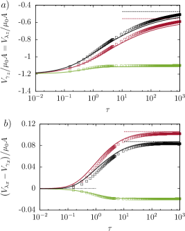
Figure 4: (Color online) The scaled particle velocities perpendicular to the membrane ($a$) and relative to each other ($b$) versus the scaled time for a constant force acting downward on both particles near a membrane endowed with only shearing (green), only bending (red) or both rigidities (black). Solid lines are the analytical predictions as given by Eq. (23), symbols are obtained by boundary-integral simulations. Horizontal dotted and dashed lines stand for the bulk and vanishing frequency limits respectively.

A situation in which hydrodynamic interactions are particularly relevant is the steady approach of two particles towards an interface, such as e.g. drug molecules approaching a cell membrane, reactant species approaching a catalyst interface, charged colloids being attracted by an oppositely charged membrane, etc. For hard walls, it is known that hydrodynamic interactions in this case are repulsive Dufresne et al. (2000); Squires and Brenner (2000); Swan and Brady (2007) leading to the dispersion of particles on the surface. Near elastic membranes, the different signs of the bending and shear contributions to the pair-mobility in Fig. 3 $b)$ point to a much more complex scenario including the possibility of particle attraction.

The physical situation of two particles being initially located at $z=z_{0}$ and suddenly set into motion towards the interface is described by a Heaviside step function force $\bm{F}(t)=\bm{A}\theta(t)$. Its Fourier transform to the frequency domain reads Bracewell (1999)

$$\bm{F}(\omega)=\left(\pi\delta(\omega)-\frac{i}{\omega}\right)\bm{A}\,.$$

Using the general form of Eq. (21), the scaled particle velocity in the temporal domain is then given by

$$\frac{V(\tau)}{\mu_{0}A}=\left(b+\int_{0}^{\infty}\frac{\varphi_{1}(u)}{\varphi_{2}(u)}\left(1-e^{-\varphi_{2}(u)\tau}\right)\mathrm{d}u\right)\theta(\tau)\,,$$ (23)

where $\tau:=t/T$ is a dimensionless time. At larger times, the exponential in Eq. (23) can be neglected compared to one. In this way, we recover the steady velocity near a hard-wall.

In corresponding BIM simulations, a constant force of small amplitude towards the wall is applied on both particles in order to retain the system symmetry. At the end of the simulations, the vertical position of the particles changes by about 8 % compared to their initial positions $z_{0}$.

In Fig. 4 $a)$ we show the time dependence of the vertical velocity which at first increases and then approaches its steady-state value. Figure 4 $b)$ shows the relative velocity between the two particles: clearly, the motion is attractive for a membrane with negligible bending resistance (such as a typical artificial capsule) which is the opposite of the behavior near a membrane with only bending resistance (such as a vesicle) or a hard wall.

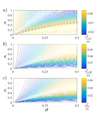
Figure 5: (Color online) Contour diagram $(\epsilon,\sigma)$ of the shearing $(a)$ and bending $(b)$ contribution in the vanishing frequency limit in the $xz$ pair-mobility as stated by Eq. (49d) for shearing and by Eq. (50d) for bending. $c)$ is the same contour near a hard-wall as given by Eq. (22d). The perturbation solution given by Eq. (24) is presented as circles in $(a)$. Contrary to a membrane with bending resistance and to a hard wall, the mobility changes sign near a membrane with shearing resistance. This sign change directly reflects the physically observable situation as the bulk contribution for the $xz$ pair-mobility is zero.

In order to illustrate more clearly for which wall and particle distances a repulsion/attraction is expected we show in Fig. 5 the pair-mobility correction for the shear $\Delta\mu^{\mathrm{P}}_{xz,\mathrm{S}}$ and bending $\Delta\mu^{\mathrm{P}}_{xz,\mathrm{B}}$ contributions in the $(\epsilon,\sigma)$ plane. To reduce the parameter space and to bring out the considered effects most clearly, we consider the idealized limit $\omega\to 0$. In this limit, the contributions become independent of the elastic moduli since $\omega\to 0$ directly implies that $\beta,\beta_{B}\to 0$ meaning that even infinitesimally small shearing and bending resistances would make the membrane behave identical to the hard wall. This unphysical behavior is remedied in a realistic situation where a small bending resistance will lead to a correspondingly large time scale $T_{\mathrm{B}}$ and thus to a long-lived transient regime as given by Eq. (23) and shown in the Supporting Information. Therefore, the contours shown in Fig. 5 faithfully represent the behavior of membranes with small bending (Fig. 5 $a)$) or small shear (Fig. 5 $b)$) resistance. The corresponding equations can be found in Appendix B.

By equating Eq. (49d) to zero and solving the resulting equation perturbatively, the threshold lines where the shearing contribution changes sign are given up to fifth order in $\sigma$ by

$$\epsilon_{\mathrm{th}}=\sqrt{2}\left(\sigma-\frac{4}{3}\sigma^{3}+\frac{17}{27}\sigma^{5}\right)+\mathcal{O}(\sigma^{7})\,.$$ (24)

Eq. (24) is shown as circles in Fig. 5. The bending contribution in Fig. 5 $b)$ always has a positive sign corresponding to a repulsive interaction similar as the hard wall.

Similar changes in sign are observed for $\Delta\mu^{\mathrm{P}}_{zz,\mathrm{S}}$ for shear and $\Delta\mu^{\mathrm{P}}_{xx,\mathrm{B}}$ for bending. The corresponding contours are given in the Supporting Information. Their physical relevance, however, is less important than for $\Delta\mu^{\mathrm{P}}_{xz}$ shown in Fig. 5 as the effects may be overshadowed by the bulk values of the mobilities (which is zero only for $\mu^{\mathrm{P}}_{xz}$).

V Diffusion

The diffusive dynamics of a pair of Brownian particles is governed by the generalized Langevin equation written for each velocity component of particle $\gamma$ as Kubo (1966)

$$\begin{split}m\frac{\mathrm{d}{V_{\gamma}}_{\alpha}}{\mathrm{d}t}&=-\int_{-\infty}^{t}\zeta^{\gamma\gamma}_{\alpha\beta}(t-t^{\prime}){V_{\gamma}}_{\beta}(t^{\prime})\mathrm{d}t^{\prime}\\ &-\int_{-\infty}^{t}\zeta^{\gamma\lambda}_{\alpha\beta}(t-t^{\prime}){V_{\lambda}}_{\beta}(t^{\prime})\mathrm{d}t^{\prime}+{F_{\gamma}}_{\alpha}(t)\,.\end{split}$$ (25)

A similar equation can be written for the velocity components of the other particle $\lambda$. Here, $m$ denotes the particles’ mass, $\zeta^{\gamma\lambda}_{\alpha\beta}(t)$ stands for the time-dependent two-particle friction retardation tensor (expressed in kg/s²) and ${F_{\gamma}}_{\alpha}$ is a random force which is zero on average. By evaluating the Fourier transform of both members in Eq. (25) and using the change of variables $w=t-t^{\prime}$ together with the shift property in the time domain of Fourier transforms we get

$$\begin{split}&im\omega{V_{\gamma}}_{\alpha}(\omega)+\zeta^{\gamma\gamma}_{\alpha\beta}[\omega]{V_{\gamma}}_{\beta}(\omega)+\zeta^{\gamma\lambda}_{\alpha\beta}[\omega]{V_{\lambda}}_{\beta}(\omega)={F_{\gamma}}_{\alpha}(\omega)\,,\\ \end{split}$$ (26)

where $\zeta^{\gamma\lambda}_{\alpha\beta}[\omega]$ and $\zeta^{\gamma\gamma}_{\alpha\beta}[\omega]$ are the Fourier-Laplace transforms of the retardation function defined as

$$\zeta^{\gamma\lambda}_{\alpha\beta}[\omega]:=\int_{0}^{\infty}\zeta^{\gamma\lambda}_{\alpha\beta}(t)e^{-i\omega t}\mathrm{d}t\,,$$ (27)

and analogously for $\zeta^{\gamma\gamma}_{\alpha\beta}[\omega]$.

In the following, we shall consider the overdamped regime for which the particles are massless $(m=0)$. Solving Eq. (26) for the particle velocities and equating with the definition of the mobilities,

$${V_{\gamma}}_{\alpha}(\omega) =\mu_{\alpha\beta}^{\gamma\gamma}(\omega){F_{\gamma}}_{\beta}(\omega)+\mu_{\alpha\beta}^{\gamma\lambda}(\omega){F_{\lambda}}_{\beta}(\omega)\,,$$ (28a)

$${V_{\lambda}}_{\alpha}(\omega) =\mu_{\alpha\beta}^{\lambda\lambda}(\omega){F_{\lambda}}_{\beta}(\omega)+\mu_{\alpha\beta}^{\lambda\gamma}(\omega){F_{\gamma}}_{\beta}(\omega)\,,$$ (28b)

leads to expressions of the mobilities in terms of the friction coefficients:

$$\mu^{\mathrm{S}}_{xx}(\omega) =\frac{\zeta_{xx}^{\mathrm{S}}\zeta_{zz}^{\mathrm{P}}}{({\zeta_{xx}^{\mathrm{S}}}^{2}-{\zeta_{xx}^{\mathrm{P}}}^{2})\zeta_{zz}^{\mathrm{P}}-\zeta_{xx}^{\mathrm{P}}{\zeta_{xz}^{\mathrm{P}}}^{2}}\,,$$

$$\mu^{\mathrm{P}}_{xx}(\omega) =-\frac{\zeta_{xx}^{\mathrm{P}}\zeta_{zz}^{\mathrm{P}}}{({\zeta_{xx}^{\mathrm{S}}}^{2}-{\zeta_{xx}^{\mathrm{P}}}^{2})\zeta_{zz}^{\mathrm{P}}-\zeta_{xx}^{\mathrm{P}}{\zeta_{xz}^{\mathrm{P}}}^{2}}\,,$$

$$\mu^{\mathrm{S}}_{yy}(\omega) =\frac{\zeta_{yy}^{\mathrm{S}}}{{\zeta_{yy}^{\mathrm{S}}}^{2}-{\zeta_{yy}^{\mathrm{P}}}^{2}}\,,$$

$$\mu^{\mathrm{P}}_{yy}(\omega) =-\frac{\zeta_{yy}^{\mathrm{P}}}{{\zeta_{yy}^{\mathrm{S}}}^{2}-{\zeta_{yy}^{\mathrm{P}}}^{2}}\,.$$

$$\mu^{\mathrm{S}}_{zz}(\omega) =\frac{\zeta_{xx}^{\mathrm{S}}\zeta_{zz}^{\mathrm{S}}}{({\zeta_{zz}^{\mathrm{S}}}^{2}-{\zeta_{zz}^{\mathrm{P}}}^{2})\zeta_{xx}^{\mathrm{S}}-\zeta_{zz}^{\mathrm{S}}{\zeta_{xz}^{\mathrm{P}}}^{2}}\,,$$

$$\mu^{\mathrm{P}}_{zz}(\omega) =-\frac{\zeta_{xx}^{\mathrm{S}}\zeta_{zz}^{\mathrm{P}}}{({\zeta_{zz}^{\mathrm{S}}}^{2}-{\zeta_{zz}^{\mathrm{P}}}^{2})\zeta_{xx}^{\mathrm{S}}-\zeta_{zz}^{\mathrm{S}}{\zeta_{xz}^{\mathrm{P}}}^{2}}\,,$$

$$\mu^{\mathrm{P}}_{xz}(\omega) =-\frac{\zeta_{zz}^{\mathrm{S}}\zeta_{xz}^{\mathrm{P}}}{({\zeta_{zz}^{\mathrm{S}}}^{2}-{\zeta_{zz}^{\mathrm{P}}}^{2})\zeta_{xx}^{\mathrm{S}}-\zeta_{zz}^{\mathrm{S}}{\zeta_{xz}^{\mathrm{P}}}^{2}}\,,$$

where the brackets [ ] are dropped out for the sake of clarity. Similar as for the mobilities, the self- and pair components of the retardation function are denoted by $\zeta_{\alpha\beta}^{\gamma\gamma}=\zeta_{\alpha\beta}^{\lambda\lambda}=\zeta_{\alpha\beta}^{\mathrm{S}}$ and $\zeta_{\alpha\beta}^{\gamma\lambda}=\zeta_{\beta\alpha}^{\lambda\gamma}=\zeta_{\alpha\beta}^{\mathrm{P}}$, respectively. Note that $\zeta_{xx}^{\mathrm{P}}\zeta_{zz}^{\mathrm{S}}=\zeta_{xx}^{\mathrm{S}}\zeta_{zz}^{\mathrm{P}}$ so that $\mu^{\mathrm{S}}_{xz}=0$ as required by symmetry.

According to the fluctuation-dissipation theorem, the frictional and random forces are related via Kubo, Toda, and Hashitsume (1985)[p. 33]Kheifets et al. (2014)

$$\langle F_{\gamma}(\omega)\overline{F_{\lambda}(\omega^{\prime})}\rangle=k_{\mathrm{B}}T\left(\zeta_{\alpha\beta}^{\gamma\lambda}[\omega]+\overline{\zeta_{\alpha\beta}^{\gamma\lambda}[\omega]}\right)\delta(\omega-\omega^{\prime})\,,$$ (30)

and analogously for the $\gamma\gamma$ component, where $k_{\mathrm{B}}$ is the Boltzmann constant and $T$ is the absolute temperature of the system.

Multiplying Eq. (28a) by its complex conjugate, taking the ensemble average and using Eq. (30), it can be shown that the velocity power spectrum obeys the relation

$${\mathcal{P}_{\mathrm{V}}}_{\alpha\beta}^{\mathrm{S}}(\omega)=k_{\mathrm{B}}T\left(\mu^{\mathrm{S}}_{\alpha\beta}(\omega)+\overline{\mu^{\mathrm{S}}_{\alpha\beta}(\omega)}\right)\,.$$ (31)

Next, by considering both Eqs. (28a) and (28b) together with Eq. (30) we find in a similar fashion

$${\mathcal{P}_{\mathrm{V}}}_{\alpha\beta}^{\mathrm{P}}(\omega)=k_{\mathrm{B}}T\left(\mu^{\mathrm{P}}_{\alpha\beta}(\omega)+\overline{\mu^{\mathrm{P}}_{\alpha\beta}(\omega)}\right)\,.$$ (32)

According to the Wiener-Khinchin-Einstein theorem, the velocity auto/cross-correlation functions can directly be obtained from the temporal inverse Fourier transform as Kubo, Toda, and Hashitsume (1985)

$${\phi}_{\alpha\beta}^{\gamma\lambda}(t)=\frac{k_{\mathrm{B}}T}{2\pi}\int_{-\infty}^{\infty}\left(\mu^{\gamma\lambda}_{\alpha\beta}(\omega)+\overline{\mu^{\gamma\lambda}_{\alpha\beta}(\omega)}\right)e^{i\omega t}\mathrm{d}\omega\,.$$ (33)

It can be shown using the residue theorem (Kubo, Toda, and Hashitsume, 1985, p. 34) that the integral over the second term in Eq. (33) vanishes if the mobility is an analytic function for $\operatorname{Im}(\omega)<0$. The present mobilities all fulfill this condition as can be seen by their general form in Eq. (21).

Most commonly, diffusion is studied in terms of the mean-square displacement (MSD) which can be calculated from the correlation function as (Kubo, Toda, and Hashitsume, 1985, p. 37)

$$\langle\Delta{r_{\gamma}}_{\alpha}(t)\Delta{r_{\lambda}}_{\beta}(t)\rangle=2\int_{0}^{t}(t-s){\phi}_{\alpha\beta}^{\gamma\lambda}(s)\mathrm{d}s\,,$$ (34)

where $\Delta{r_{\gamma}}_{\alpha}$ denotes the displacement of the particle $\gamma$ in the direction $\alpha$. Furthermore, we define the time-dependent pair-diffusion tensor as

$$D_{\alpha\beta}^{\gamma\lambda}(t):=\frac{\langle\Delta{r_{\gamma}}_{\alpha}(t)\Delta{r_{\lambda}}_{\beta}(t)\rangle}{2t}\,.$$ (35)

Analogous relations to Eqs. (33)-(35) hold for the $\gamma\gamma$ component. We now consider the collective motions of the center of mass $\bm{\rho}:=\bm{r}_{\lambda}+\bm{r}_{\gamma}$ as well as the relative motion $\bm{h}:=\bm{r}_{\lambda}-\bm{r}_{\gamma}$ with the corresponding diagonal pair-diffusion tensor

$$D_{\alpha\alpha}^{C,R}=2\left(D_{\alpha\alpha}^{\mathrm{S}}\pm D_{\alpha\alpha}^{\mathrm{P}}\right)\,,$$ (36)

where the positive sign applies for the collective mode of motion and the negative sign to the relative mode. In the absence of the membrane, Eqs. (36) reduces to the generalization of the Einstein relation as calculated by Batchelor Batchelor (1976) for the relative mode, namely

$$\frac{D_{zz}^{\mathrm{R}}}{2D_{0}}=1-\frac{3}{4}\sigma-\frac{\sigma^{3}}{2}\,,\quad\frac{D_{xx}^{\mathrm{R}}}{2D_{0}}=1-\frac{3}{2}\sigma+\sigma^{3}\,,$$ (37)

where $D_{0}:=\mu_{0}k_{\mathrm{B}}T$ is the diffusion coefficient. The collective diffusion coefficients read

$$\frac{D_{zz}^{\mathrm{C}}}{2D_{0}}=1+\frac{3}{4}\sigma+\frac{\sigma^{3}}{2}\,,\quad\frac{D_{xx}^{\mathrm{C}}}{2D_{0}}=1+\frac{3}{2}\sigma-\sigma^{3}\,,$$ (38)

V.1 Self-diffusion for finite-sized particles

From Eqs. (33)-(35) we first obtain the scaled self-diffusion coefficient for the motion of a single particle perpendicular to the membrane,

$$\begin{split}\frac{D_{zz}^{\mathrm{S}}}{D_{0}}&=1-\frac{3}{32}\frac{\tau_{\mathrm{S}}(3B+2\tau_{\mathrm{S}})}{(B+\tau_{\mathrm{S}})^{2}}\epsilon+\frac{\tau_{\mathrm{S}}}{16}\frac{3\tau_{\mathrm{S}}^{2}+8B\tau_{\mathrm{S}}+6B^{2}}{(B+\tau_{\mathrm{S}})^{3}}\epsilon^{3}\\ &-\frac{\tau_{\mathrm{S}}}{64}\frac{4\tau_{\mathrm{S}}^{3}+15B\tau_{\mathrm{S}}^{2}+20B^{2}\tau_{\mathrm{S}}+10B^{3}}{(B+\tau_{\mathrm{S}})^{4}}\epsilon^{5}\,\\ &-\frac{\epsilon}{12}\int_{0}^{\infty}\left(3+3u-\epsilon^{2}u^{2}\right)^{2}\left(1-\frac{1-e^{-{\tau_{\mathrm{B}}u^{3}}}}{\tau_{\mathrm{B}}u^{3}}\right)e^{-2u}\mathrm{d}u\,,\end{split}$$ (39)

where $\tau_{\mathrm{S}}:=t/T_{\mathrm{S}}$ and $\tau_{\mathrm{B}}:=t/T_{\mathrm{B}}$ are dimensionless times for shearing and bending, respectively.

For motion parallel to the membrane the scaled self-diffusion coefficient reads

$$\begin{split}\frac{D_{xx}^{\mathrm{S}}}{D_{0}}&=1-\frac{3}{64}\bigg{(}\frac{(2\tau_{\mathrm{S}}+3B)(5\tau_{\mathrm{S}}+4B)}{(\tau_{\mathrm{S}}+B)^{2}}-\frac{4B}{\tau_{\mathrm{S}}}\ln\left(1+\frac{\tau_{\mathrm{S}}}{B}\right)\\ &-\frac{16}{\tau_{\mathrm{S}}}\ln\left(1+\frac{\tau_{\mathrm{S}}}{2}\right)\bigg{)}\epsilon+\frac{\tau_{\mathrm{S}}}{32}\frac{\tau_{\mathrm{S}}^{2}+3B\tau_{\mathrm{S}}+3B^{2}}{(\tau_{\mathrm{S}}+B)^{3}}\epsilon^{3}\\ &-\frac{\tau_{\mathrm{S}}}{128}\frac{4\tau_{\mathrm{S}}^{3}+15B\tau_{\mathrm{S}}^{2}+20B^{2}\tau_{\mathrm{S}}+10B^{3}}{(\tau_{\mathrm{S}}+B)^{4}}\epsilon^{5}\,\\ &-\frac{\epsilon}{12}\int_{0}^{\infty}\left(3-\epsilon^{2}u\right)^{2}\left(u^{2}-\frac{1-e^{-{\tau_{\mathrm{B}}u^{3}}}}{\tau_{\mathrm{B}}u}\right)e^{-2u}\mathrm{d}u\,.\end{split}$$ (40)

We mention that Eqs. (39) and (40) correspond to leading order in $\epsilon$ to the ones reported in our earlier work Daddi-Moussa-Ider, Guckenberger, and Gekle (2016a). For long times, the perpendicular velocity auto-correlation function $\phi_{zz,\mathrm{S}}^{\mathrm{S}}$ decays as $t^{-4}$ whereas the bending part $\phi_{zz,\mathrm{B}}^{\mathrm{S}}$ as $t^{-4/3}$. For parallel motion, both the shearing and bending parts in the velocity auto-correlation function have a long-time tail of $t^{-2}$.

V.2 Pair-diffusion for finite-sized particles

The pair-diffusion coefficients are readily obtained by plugging Eqs. (20a) through (20d) into Eqs. (33)-(35):

$$\frac{D_{zz}^{\mathrm{P}}}{D_{0}} =\frac{3\sigma}{4}+\frac{\sigma^{3}}{2}-\frac{\sigma}{12\xi^{5/2}}\int_{0}^{\infty}\left(u\Lambda^{2}\Pi_{\mathrm{S}}+\frac{2\Gamma_{-}^{2}}{u^{3}}\Pi_{\mathrm{B}}\right)\chi_{0}e^{-2u}\mathrm{d}u\,,$$ (41a)

$$\frac{D_{xx}^{\mathrm{P}}}{D_{0}} =\frac{3\sigma}{2}-\sigma^{3}-\sigma\int_{0}^{\infty}\left(\frac{1}{24\xi^{5/2}}\left(-\xi^{1/2}\chi_{1}+2u\chi_{0}\right)\left(\Gamma_{+}^{2}\Pi_{\mathrm{S}}+2\Lambda^{2}\Pi_{\mathrm{B}}\right)+\frac{3\chi_{1}}{2}\Pi_{\mathrm{S}}^{\prime}\right)\frac{e^{-2u}}{u^{2}}\mathrm{d}u\,,$$ (41b)

$$\frac{D_{yy}^{\mathrm{P}}}{D_{0}} =\frac{3\sigma}{4}+\frac{\sigma^{3}}{2}-\sigma\int_{0}^{\infty}\left(\frac{\chi_{1}}{24\xi^{2}}\left(\Gamma_{+}^{2}\Pi_{\mathrm{S}}+2\Lambda^{2}\Pi_{\mathrm{B}}\right)+\frac{3\Pi_{\mathrm{S}}^{\prime}}{2\xi^{1/2}}\left(-\xi^{1/2}\chi_{1}+2u\chi_{0}\right)\right)\frac{e^{-2u}}{u^{2}}\mathrm{d}u\,,$$ (41c)

$$\frac{D_{xz}^{\mathrm{P}}}{D_{0}} =\frac{\sigma}{12\xi^{5/2}}\int_{0}^{\infty}\left(\Gamma_{+}\Pi_{\mathrm{S}}+\frac{2\Gamma_{-}\Pi_{\mathrm{B}}}{u^{2}}\right)\chi_{1}\Lambda e^{-2u}\mathrm{d}u\,,$$ (41d)

where we define

$$\Pi_{\mathrm{S}}:=\frac{Be^{-\frac{2u\tau_{\mathrm{S}}}{B}}+2u\tau_{\mathrm{S}}-B}{\tau_{\mathrm{S}}}\,,\quad\Pi_{\mathrm{S}}^{\prime}:=\frac{e^{-\tau_{\mathrm{S}}u}+\tau_{\mathrm{S}}u-1}{\tau_{\mathrm{S}}}\,,\quad\Pi_{\mathrm{B}}:=\frac{e^{-\tau_{\mathrm{B}}u^{3}}+\tau_{\mathrm{B}}u^{3}-1}{\tau_{\mathrm{B}}}\,.$$

We observe that the $xx$, $yy$ and $zz$ cross-correlation functions have the same large time behavior as their corresponding auto-correlation functions. For the component $\phi_{xz}^{\mathrm{P}}$, the shearing and bending related parts have large-time tails of $t^{-4}$ and $t^{-2}$, respectively.

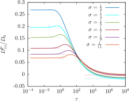
Figure 6: (Color online) The $zz$ component of the scaled pair-diffusion tensor versus the scaled time as given by Eq. (41a) for different values of $\sigma$ with the parameters of Fig. 3. Horizontal dotted and dashed lines represent the bulk and hard-wall limits, respectively. For large inter-particle distances (small $\sigma$) a short superdiffusive regime is observed.

Fig. 6 shows the variations of the $zz$ component of the scaled pair-diffusion coefficient as stated by Eq. (41a) upon varying $\sigma$. We observe that as $\sigma$ decreases, i.e. when the two particles stand further apart, the pair-diffusion coefficient can rise and exceed the bulk value for intermediate time scales as hinted on already by the pair-mobility around $\beta\sim 1$ (cf. inset of Fig. 3 $a$). Such behavior is a clear signature of a short-lived superdiffusive regime.

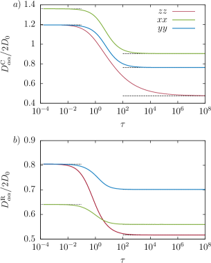
Figure 7: (Color online) The scaled collective $(a)$ and relative $(b)$ diffusion coefficients as defined by Eq. (36) versus the scaled time. The horizontal dotted and dashed lines correspond to the bulk and hard-wall limits, respectively.

In Fig. 7 we show the variations of the scaled collective and relative diffusion coefficients as defined by Eq. (36), versus the scaled time $\tau$, using the parameters of Fig. 3. At shorter time scales, the particle pair exhibits a normal bulk diffusion, since the motion is hardly affected by the presence of the membrane. As a result, the diffusion coefficients are the same as calculated by Batchelor and given by Eq. (37). As the time increases, both diffusion coefficients’ curves bend down substantially to asymptotically approach the diffusion coefficients near a hard-wall.

VI Conclusions

We have investigated the hydrodynamic interaction of a finite-size particle pair nearby an elastic membrane endowed with shear and bending rigidity. Using multipole expansions together with Faxén’s law, we have provided analytical expressions for the frequency-dependent self- and pair-mobilities. We have demonstrated that shearing and bending contributions may give positive or negative contributions to particle pair-mobilities depending on the inter-particle distance and the pair location above the membrane. Most prominently, we have found that two particles approaching a membrane with only shearing resistance (as is typically assumed for elastic capsules) may experience hydrodynamic attraction in contrast to the well-known case of a hard wall where the interaction is repulsive. This unexpected effect will facilitate chemical reactions near the surface and may possibly even lead to the formation of particle clusters near elastic membranes. On the other hand, membranes with bending resistance (such as vesicles) induce repulsive interactions similar to the hard wall. All our theoretical mobilities are validated by detailed boundary integral simulations.

Using the frequency-dependent particle mobilities, we have computed self- and pair-diffusion coefficients. Most commonly, relative and collective pair-diffusion is subdiffusive on intermediate time scales similar to earlier observations on the diffusion of a single particle Daddi-Moussa-Ider, Guckenberger, and Gekle (2016a). A notable exception is the $zz$-component of the pair-mobility tensor which for certain parameters and frequencies surpasses its corresponding bulk value. This induces a short-lasting superdiffusive regime in the corresponding mean-square-displacement.

Appendix A Derivation of Green’s functions

In this appendix, we briefly sketch the derivation of the Green’s functions in the presence of an elastic membrane, as stated by Eqs. (12a) through (12d) of the main text. For the solution of the steady Stokes equations Eqs. (10) and (11), we use a two-dimensional Fourier transform technique. The variables $x$ and $y$ are transformed into the wavevector components $q_{x}$ and $q_{y}$. Here we use the convention with a negative exponent for the forward Fourier transforms. The transformed equations read

$$-q^{2}\tilde{v}_{x}+\tilde{v}_{x,zz}+iq_{x}\tilde{p}+\tilde{F}_{x}\delta(z-z_{0}) =0\,,$$

$$-q^{2}\tilde{v}_{y}+\tilde{v}_{y,zz}+iq_{y}\tilde{p}+\tilde{F}_{y}\delta(z-z_{0}) =0\,,$$

$$-q^{2}\tilde{v}_{z}+\tilde{v}_{z,zz}-\tilde{p}_{,z}+\tilde{F}_{z}\delta(z-z_{0}) =0\,,$$

$$-iq_{x}\tilde{v}_{x}-iq_{y}\tilde{v}_{y}+\tilde{v}_{z,z} =0\,,$$

where a comma in indices denotes the spatial derivative with respect to the following coordinate.

We introduce a new orthonormal system in which the Fourier transformed vectorial quantities are decomposed into longitudinal, transverse and normal components, denoted by $\tilde{v}_{l}$, $\tilde{v}_{t}$ and $\tilde{v}_{z}$ respectively. The corresponding orthonormal in-plane unit vector basis are

$$\bm{q}_{l}:=\frac{q_{x}}{q}\bm{e}_{x}+\frac{q_{y}}{q}\bm{e}_{y}\,,\quad\bm{q}_{t}:=\frac{q_{y}}{q}\bm{e}_{x}-\frac{q_{x}}{q}\bm{e}_{y}\,,$$ (42)

where $q:=\sqrt{q_{x}^{2}+q_{y}^{2}}$ is the wavenumber. After transformation, the momentum equations become Bickel (2007)

$$q^{2}\tilde{v}_{t}-\tilde{v}_{t,zz} =\frac{\tilde{F}_{t}}{\eta}\delta(z-z_{0})\,,$$ (43a)

$$\tilde{v}_{z,zzzz}-2q^{2}\tilde{v}_{z,zz}+q^{4}\tilde{v}_{z} =\frac{q^{2}\tilde{F}_{z}}{\eta}\delta(z-z_{0})$$

$$\quad+\frac{iq\tilde{F}_{l}}{\eta}\delta^{\prime}(z-z_{0})\,,$$ (43b)

where $\delta^{\prime}$ is the derivative of the Dirac delta function. The longitudinal component $\tilde{v}_{l}$ is readily determined from $\tilde{v}_{z}$ via the incompressibility equation (11) such that

$$\tilde{v}_{l}=\frac{i\tilde{v}_{z,z}}{q}\,.$$ (44)

According to the Skalak Skalak et al. (1973) and Helfrich Helfrich (1973) models, the linearized tangential and normal traction jumps across the membrane are related to the membrane displacement field $\bm{u}$ at $z=0$ by Daddi-Moussa-Ider, Guckenberger, and Gekle (2016a)

$$[\sigma_{z\alpha}] =-\frac{\kappa_{\mathrm{S}}}{3}\left(\Delta_{\parallel}u_{\alpha}+(1+2C)e_{,\alpha}\right)\,,\quad\alpha\in\{x,y\}\,,$$ (45a)

$$\leavevmode\nobreak\ [\sigma_{zz}] =\kappa_{\mathrm{B}}\Delta_{\parallel}^{2}u_{z}\,,$$ (45b)

where the notation $[w]:=w(0^{+})-w(0^{-})$ designates the jump of the quantity $w$ across the membrane. Here $C:=\kappa_{\mathrm{A}}/\kappa_{\mathrm{S}}$ is a dimensionless number representing the ratio of the area expansion modulus to shear modulus, and $\kappa_{\mathrm{B}}$ is the membrane bending modulus. $\Delta_{\parallel}:=\partial_{,xx}+\partial_{,yy}$ denotes the Laplace-Beltrami operator along the membrane and $e:=u_{x,x}+u_{y,y}$ is the dilatation function, mathematically defined as the trace of the in-plane strain tensor.

The membrane displacement $\bm{u}$ as appearing in Eqs. (45a) and (45b) is related to the fluid velocity by the no-slip boundary condition at the undisplaced membrane which reads

$$\tilde{v}_{\alpha}=i\omega\tilde{u}_{\alpha}|_{z=0}\,.$$ (46)

After solving the transformed equations (43a), (43b) and (44) and properly applying the boundary conditions at the membrane, we find that the diagonal components of the Green’s function for $z\geq 0$ read

$$\tilde{\mathcal{G}}_{zz} =\frac{1}{4\eta q}\bigg{(}\left(1+q|z-z_{0}|\right)e^{-q|z-z_{0}|}$$

$$+\left(\frac{i\alpha zz_{0}q^{3}}{1-i\alpha q}+\frac{i\alpha_{\mathrm{B}}^{3}q^{3}(1+qz)(1+qz_{0})}{1-i\alpha_{\mathrm{B}}^{3}q^{3}}\right)e^{-q(z+z_{0})}\bigg{)}\,,$$

$$\tilde{\mathcal{G}}_{ll} =\frac{1}{4\eta q}\bigg{(}(1-q|z-z_{0}|)e^{-q|z-z_{0}|}$$

$$+\left(\frac{i\alpha q(1-qz_{0})(1-qz)}{1-i\alpha q}+\frac{izz_{0}\alpha_{\mathrm{B}}^{3}q^{5}}{1-i\alpha_{\mathrm{B}}^{3}q^{3}}\right)e^{-q(z+z_{0})}\bigg{)}\,,$$

$$\tilde{\mathcal{G}}_{tt} =\frac{1}{2\eta q}\left(e^{-q|z-z_{0}|}+\frac{iB\alpha q}{2-iB\alpha q}e^{-q(z+z_{0})}\right)\,,$$

and the off-diagonal component $\tilde{\mathcal{G}}_{lz}$ reads

$$\tilde{\mathcal{G}}_{lz} =\frac{i}{4\eta q}\bigg{(}-q(z-z_{0})e^{-q|z-z_{0}|}$$

$$+\left(\frac{i\alpha z_{0}q^{2}(1-qz)}{1-i\alpha q}-\frac{i\alpha_{\mathrm{B}}^{3}zq^{4}(1+qz_{0})}{1-i\alpha_{\mathrm{B}}^{3}q^{3}}\right)e^{-q(z+z_{0})}\bigg{)}\,,$$

where $\alpha:=\kappa_{\mathrm{S}}/(3B\eta\omega)$ is a characteristic length scale for shearing and area expansion with $B:=2/(1+C)$, and $\alpha_{\mathrm{B}}:=(\kappa_{\mathrm{B}}/(4\eta\omega))^{1/3}$ is a characteristic length scale for bending. Furthermore, $\tilde{\mathcal{G}}_{tz}=\tilde{\mathcal{G}}_{zt}=0$ because of the decoupled nature of Eqs. (43a) and (43b). Employing the transformation equations (42) back to the usual Cartesian basis, we obtain

$$\tilde{\mathcal{G}}_{xx}(\bm{q},z,\omega) =\tilde{\mathcal{G}}_{ll}(q,z,\omega)\cos^{2}\phi+\tilde{\mathcal{G}}_{tt}(q,z,\omega)\sin^{2}\phi\,,$$

$$\tilde{\mathcal{G}}_{yy}(\bm{q},z,\omega) =\tilde{\mathcal{G}}_{ll}(q,z,\omega)\sin^{2}\phi+\tilde{\mathcal{G}}_{tt}(q,z,\omega)\cos^{2}\phi\,,$$

$$\tilde{\mathcal{G}}_{xz}(\bm{q},z,\omega) =\tilde{\mathcal{G}}_{lz}(q,z,\omega)\cos\phi\,,$$

where $\phi:=\arctan(q_{y}/q_{x})$.

The components $\tilde{\mathcal{G}}_{yz}$ and $\tilde{\mathcal{G}}_{zy}$ are irrelevant for our discussion because the resulting mobilities vanish, thus they are omitted here. In addition, the component $\tilde{\mathcal{G}}_{zx}$ leads to the same mobility as $\tilde{\mathcal{G}}_{xz}$ because of the symmetry of the mobility tensor. Furthermore, we define

$$\tilde{\mathcal{G}}_{\pm}(q,z,\omega):=\tilde{\mathcal{G}}_{tt}(q,z,\omega)\pm\tilde{\mathcal{G}}_{ll}(q,z,\omega)\,.$$

Eqs. (12a)-(12d) of the main text follow immediately after performing the two dimensional inverse spatial Fourier transform of the Green’s function Bracewell (1999).

Appendix B Vanishing frequency behavior

In the following, analytical expressions of the shearing and bending related parts in the particle self- and pair-mobilities are provided in the vanishing frequency limit.

B.1 Self mobilities

By taking the vanishing frequencies limit in Eqs. (15a) and (15b), the shearing and bending related corrections for the perpendicular motion read

$$\lim_{\beta\to 0}\frac{\Delta\mu_{zz,\mathrm{S}}^{\mathrm{S}}}{\mu_{0}} =-\frac{3}{16}\epsilon+\frac{3}{16}\epsilon^{3}-\frac{1}{16}\epsilon^{5}\,,$$

$$\lim_{\beta_{\mathrm{B}}\to 0}\frac{\Delta\mu_{zz,\mathrm{B}}^{\mathrm{S}}}{\mu_{0}} =-\frac{15}{16}\epsilon+\frac{5}{16}\epsilon^{3}-\frac{1}{16}\epsilon^{5}\,,$$

leading to the hard-wall limit Eq. (16) after summing up both contributions term by term. Similarly, for the parallel motion, by taking the vanishing frequency limit in Eqs. (17a) and (17b) we get

$$\lim_{\beta\to 0}\frac{\Delta\mu_{xx,\mathrm{S}}^{\mathrm{S}}}{\mu_{0}} =-\frac{15}{32}\epsilon+\frac{1}{32}\epsilon^{3}-\frac{1}{32}\epsilon^{5}\,,$$

$$\lim_{\beta_{\mathrm{B}}\to 0}\frac{\Delta\mu_{xx,\mathrm{B}}^{\mathrm{S}}}{\mu_{0}} =-\frac{3}{32}\epsilon+\frac{3}{32}\epsilon^{3}-\frac{1}{32}\epsilon^{5}\,,$$

which also give the hard-wall limit Eq. (18) when summing up both parts.

B.2 Pair mobilities

By considering independently the shearing and bending related parts in the pair-mobility corrections as given by Eqs. (20a) through (20d), and taking the vanishing frequency limit, we obtain for the shearing part

$$\lim_{\beta\to 0}\frac{\Delta\mu_{zz,\mathrm{S}}^{\mathrm{P}}}{\mu_{0}} =-\frac{3}{16}\frac{\xi(2\xi-1)}{(1+\xi)^{5/2}}\sigma+\frac{3}{4}\frac{\xi(2\xi-3)}{(1+\xi)^{7/2}}\sigma^{3}$$

$$-\frac{2\xi^{2}-6\xi+\frac{3}{4}}{(1+\xi)^{9/2}}\sigma^{5}\,,$$ (49a)

$$\lim_{\beta\to 0}\frac{\Delta\mu_{xx,\mathrm{S}}^{\mathrm{P}}}{\mu_{0}} =-\frac{3}{16}\frac{5\xi^{2}+10\xi+8}{(1+\xi)^{5/2}}\sigma+\frac{1}{4}\frac{\xi^{2}-10\xi+4}{(1+\xi)^{7/2}}\sigma^{3}$$

$$-\frac{\xi^{2}-\frac{27}{4}\xi+1}{(1+\xi)^{9/2}}\sigma^{5}\,,$$ (49b)

$$\lim_{\beta\to 0}\frac{\Delta\mu_{yy,\mathrm{S}}^{\mathrm{P}}}{\mu_{0}} =-\frac{3}{16}\frac{5\xi+4}{(1+\xi)^{3/2}}\sigma+\frac{1}{4}\frac{\xi-2}{(1+\xi)^{5/2}}\sigma^{3}$$

$$-\frac{\xi-\frac{1}{4}}{(1+\xi)^{7/2}}\sigma^{5}\,,$$ (49c)

$$\lim_{\beta\to 0}\frac{\Delta\mu_{xz,\mathrm{S}}^{\mathrm{P}}}{\mu_{0}} =\frac{3}{16}\frac{(\xi-2)\xi^{1/2}}{(1+\xi)^{5/2}}\sigma-\frac{3}{4}\frac{(3\xi-2)\xi^{1/2}}{(1+\xi)^{7/2}}\sigma^{3}$$

$$+\frac{5}{4}\frac{(4\xi-3)\xi^{1/2}}{(1+\xi)^{9/2}}\sigma^{5}\,,$$ (49d)

and for the bending part

$$\lim_{\beta_{\mathrm{B}}\to 0}\frac{\Delta\mu_{zz,\mathrm{B}}^{\mathrm{P}}}{\mu_{0}} =-\frac{3}{16}\frac{10\xi^{2}+11\xi+4}{(1+\xi)^{5/2}}\sigma+\frac{1}{4}\frac{10\xi^{2}-7\xi-2}{(1+\xi)^{7/2}}\sigma^{3}$$

$$-\frac{2\xi^{2}-6\xi+\frac{3}{4}}{(1+\xi)^{9/2}}\sigma^{5}\,,$$ (50a)

$$\lim_{\beta_{\mathrm{B}}\to 0}\frac{\Delta\mu_{xx,\mathrm{B}}^{\mathrm{P}}}{\mu_{0}} =-\frac{3}{16}\frac{\xi(\xi-2)}{(1+\xi)^{5/2}}\sigma+\frac{3}{4}\frac{\xi(\xi-4)}{(1+\xi)^{7/2}}\sigma^{3}$$

$$-\frac{\xi^{2}-\frac{27}{4}\xi+1}{(1+\xi)^{9/2}}\sigma^{5}\,,$$ (50b)

$$\lim_{\beta_{\mathrm{B}}\to 0}\frac{\Delta\mu_{yy,\mathrm{B}}^{\mathrm{P}}}{\mu_{0}} =-\frac{3}{16}\frac{\xi}{(1+\xi)^{3/2}}\sigma+\frac{3}{4}\frac{\xi}{(1+\xi)^{5/2}}\sigma^{3}$$

$$-\frac{\xi-\frac{1}{4}}{(1+\xi)^{7/2}}\sigma^{5}\,,$$ (50c)

$$\lim_{\beta_{\mathrm{B}}\to 0}\frac{\Delta\mu_{xz,\mathrm{B}}^{\mathrm{P}}}{\mu_{0}} =\frac{3}{16}\frac{(5\xi+2)\xi^{1/2}}{(1+\xi)^{5/2}}\sigma-\frac{15}{4}\frac{\xi^{3/2}}{(1+\xi)^{7/2}}\sigma^{3}$$

$$+\frac{5}{4}\frac{(4\xi-3)\xi^{1/2}}{(1+\xi)^{9/2}}\sigma^{5}\,.$$ (50d)

The total correction as given by Eqs. (22a) through (22d) is recovered by summing up term by term both contributions.

References

- Morrone, Li, and Berne (2012) J. A. Morrone, J. Li, and B. J. Berne, “Interplay between Hydrodynamics and the Free Energy Surface in the Assembly of Nanoscale Hydrophobes,” J. Phys. Chem. B 116, 378–389 (2012).
- Usta, Ladd, and Butler (2005) O. B. Usta, A. J. C. Ladd, and J. E. Butler, “Lattice-boltzmann simulations of the dynamics of polymer solutions in periodic and confined geometries,” J. Chem. Phys. 122, 094902 (2005).
- Wojciechowski, Szymczak, and Cieplak (2010) M. Wojciechowski, P. Szymczak, and M. Cieplak, “The influence of hydrodynamic interactions on protein dynamics in confined and crowded spaces—assessment in simple models,” Physical biology 7, 046011 (2010).
- von Hansen, Netz, and Hinczewski (2010) Y. von Hansen, R. R. Netz, and M. Hinczewski, “DNA-protein binding rates: Bending fluctuation and hydrodynamic coupling effects,” J. Chem. Phys. 132, 135103–13 (2010).
- Długosz et al. (2012) M. Długosz, J. M. Antosiewicz, P. Zieliński, and J. Trylska, “Contributions of Far-Field Hydrodynamic Interactions to the Kinetics of Electrostatically Driven Molecular Association,” J. Phys. Chem. B 116, 5437–5447 (2012).
- Ando and Skolnick (2013) T. Ando and J. Skolnick, “On the Importance of Hydrodynamic Interactions in Lipid Membrane Formation,” Biophys J 104, 96–105 (2013).
- Popel and Johnson (2005) A. S. Popel and P. C. Johnson, “Microcirculation and hemorheology,” Annu. Rev. Fluid Mech. 37, 43–69 (2005).
- Misbah and Wagner (2013) C. Misbah and C. Wagner, “Living fluids,” C. R. Physique 14, 447–450 (2013).
- Molina, Nakayama, and Yamamoto (2013) J. J. Molina, Y. Nakayama, and R. Yamamoto, “Hydrodynamic interactions of self-propelled swimmers,” Soft Matter 9, 4923–4936 (2013).
- Wensink et al. (2012) H. H. Wensink, J. Dunkel, S. Heidenreich, K. Drescher, R. E. Goldstein, H. Löwen, and J. M. Yeomans, “Meso-scale turbulence in living fluids,” Proceedings of the National Academy of Sciences 109, 14308–14313 (2012).
- Dunkel et al. (2013) J. Dunkel, S. Heidenreich, K. Drescher, H. H. Wensink, M. Bär, and R. E. Goldstein, “Fluid dynamics of bacterial turbulence,” Phys. Rev. Lett. 110, 228102 (2013).
- Lopez and Lauga (2014) D. Lopez and E. Lauga, “Dynamics of swimming bacteria at complex interfaces,” Phys. Fluids 26, 071902 (2014).
- Zöttl and Stark (2014) A. Zöttl and H. Stark, “Hydrodynamics Determines Collective Motion and Phase Behavior of Active Colloids in Quasi-Two-Dimensional Confinement,” Phys. Rev. Lett. 112, 118101–5 (2014).
- Elgeti, Winkler, and Gompper (2015) J. Elgeti, R. G. Winkler, and G. Gompper, “Physics of microswimmers—single particle motion and collective behavior: a review,” Reports on progress in physics 78, 056601 (2015).
- Guazzelli and Morris (2012) É.. Guazzelli and J. F. Morris, A physical introduction to suspension dynamics (Cambridge University Press, 2012).
- Larsen, Grier et al. (1997) A. E. Larsen, D. G. Grier, et al., “Like-charge attractions in metastable colloidal crystallites,” Nature 385, 230–233 (1997).
- Squires and Brenner (2000) T. M. Squires and M. P. Brenner, “Like-charge attraction and hydrodynamic interaction,” Phys. Rev. Lett. 85, 4976 (2000).
- Behrens and Grier (2001) S. H. Behrens and D. G. Grier, “Pair interaction of charged colloidal spheres near a charged wall,” Phys. Rev. E 64, 050401 (2001).
- Felderhof (1977) B. U. Felderhof, “Hydrodynamic interaction between two spheres,” Physica A 89, 373–384 (1977).
- Kim and Mifflin (1985) S. Kim and R. T. Mifflin, “The resistance and mobility functions of two equal spheres in low-reynolds-number flow,” Phys. Fluids 28, 2033–2045 (1985).
- Yoon and Kim (1987) B. J. Yoon and S. Kim, “Note on the direct calculation of mobility functions for two equal-sized spheres in stokes flow,” J. Fluid Mech. 185, 437–446 (1987).
- Cichocki, Felderhof, and Schmitz (1988) B. Cichocki, B. U. Felderhof, and R. Schmitz, “Hydrodynamic interactions between two spherical particles,” PhysicoChem. Hyd 10, 383–403 (1988).
- Happel and Brenner (2012) J. Happel and H. Brenner, Low Reynolds number hydrodynamics: with special applications to particulate media, Vol. 1 (Springer Science & Business Media, 2012).
- Deutch and Oppenheim (1971) J. M. Deutch and I. Oppenheim, “Molecular theory of brownian motion for several particles,” J. Chem. Phys. 54, 3547–3555 (1971).
- Batchelor (1976) G. K. Batchelor, “Brownian diffusion of particles with hydrodynamic interaction,” J. Fluid Mech. 74, 1–29 (1976).
- Ermak and McCammon (1978) D. L. Ermak and J. McCammon, “Brownian dynamics with hydrodynamic interactions,” J. Chem. Phys. 69, 1352–1360 (1978).
- Ladd (1988) A. J. C. Ladd, “Hydrodynamic interactions in a suspension of spherical particles,” J. Chem. Phys. 88, 5051–5063 (1988).
- Ekiel-Jeżewska and Felderhof (2015) M. L. Ekiel-Jeżewska and B. U. Felderhof, “Hydrodynamic interactions between a sphere and a number of small particles,” J. Chem. Phys. 142, 014904 (2015).
- Zia, Swan, and Su (2015) R. N. Zia, J. W. Swan, and Y. Su, “Pair mobility functions for rigid spheres in concentrated colloidal dispersions: Force, torque, translation, and rotation,” J. Chem. Phys. 143, 224901 (2015).
- Crocker (1997) J. C. Crocker, “Measurement of the hydrodynamic corrections to the brownian motion of two colloidal spheres,” J. Chem. Phys. 106, 2837–2840 (1997).
- Meiners and Quake (1999) J.-C. Meiners and S. R. Quake, “Direct measurement of hydrodynamic cross correlations between two particles in an external potential,” Phys. Rev. Lett. 82, 2211–2214 (1999).
- Bartlett, Henderson, and Mitchell (2001) P. Bartlett, S. I. Henderson, and S. J. Mitchell, “Measurement of the hydrodynamic forces between two polymer–coated spheres,” Philosophical Transactions of the Royal Society of London A: Mathematical, Physical and Engineering Sciences 359, 883–895 (2001).
- Henderson, Mitchell, and Bartlett (2002) S. Henderson, S. Mitchell, and P. Bartlett, “Propagation of hydrodynamic interactions in colloidal suspensions,” Phys. Rev. Lett. 88, 088302 (2002).
- Radiom et al. (2015) M. Radiom, B. Robbins, M. Paul, and W. Ducker, “Hydrodynamic interactions of two nearly touching brownian spheres in a stiff potential: Effect of fluid inertia,” Phys. Fluids 27, 022002 (2015).
- Lauga and Squires (2005) E. Lauga and T. M. Squires, “Brownian motion near a partial-slip boundary: A local probe of the no-slip condition,” Phys. Fluids 17 (2005).
- Lorentz (1907) H. A. Lorentz, “Ein allgemeiner satz, die bewegung einer reibenden flüssigkeit betreffend, nebst einigen anwendungen desselben,” Abh. Theor. Phys. 1, 23 (1907).
- MacKay and Mason (1961) G. D. M. MacKay and S. G. Mason, “Approach of a solid sphere to a rigid plane interface,” J. Colloid Sci. 16, 632–635 (1961).
- Gotoh and Kaneda (1982) T. Gotoh and Y. Kaneda, “Effect of an infinite plane wall on the motion of a spherical brownian particle,” J. Chem. Phys. 76, 3193–3197 (1982).
- Cichocki and Jones (1998) B. Cichocki and R. B. Jones, “Image representation of a spherical particle near a hard wall,” Physica A 258, 273–302 (1998).
- Franosch and Jeney (2009) T. Franosch and S. Jeney, “Persistent correlation of constrained colloidal motion,” Phys. Rev. E 79, 031402 (2009).
- Felderhof (2012) B. U. Felderhof, “Hydrodynamic force on a particle oscillating in a viscous fluid near a wall with dynamic partial-slip boundary condition,” Phys. Rev. E 85, 046303 (2012).
- Padding and Briels (2010) J. T. Padding and W. J. Briels, “Translational and rotational friction on a colloidal rod near a wall,” J. Chem. Phys. 132, 054511 (2010).
- De Corato et al. (2015) M. De Corato, F. Greco, G. D’Avino, and P. L. Maffettone, “Hydrodynamics and brownian motions of a spheroid near a rigid wall,” J. Chem. Phys. 142 (2015).
- Huang and Szlufarska (2015) K. Huang and I. Szlufarska, “Effect of interfaces on the nearby brownian motion,” Nature communications 6 (2015).
- Lee, Chadwick, and Leal (1979) S. H. Lee, R. S. Chadwick, and L. G. Leal, “Motion of a sphere in the presence of a plane interface. part 1. an approximate solution by generalization of the method of lorentz,” J. Fluid Mech. 93, 705–726 (1979).
- Berdan and Leal (1982) C. Berdan and L. G. Leal, “Motion of a sphere in the presence of a deformable interface: I. perturbation of the interface from flat: the effects on drag and torque,” J. Colloid Interface Sci. 87, 62 – 80 (1982).
- Bickel (2006) T. Bickel, “Brownian motion near a liquid-like membrane,” Eur. Phys. J. E 20, 379–385 (2006).
- Bickel (2007) T. Bickel, “Hindered mobility of a particle near a soft interface,” Phys. Rev. E 75, 041403 (2007).
- Bławzdziewicz, Ekiel-Jeżewska, and Wajnryb (2010a) J. Bławzdziewicz, M. Ekiel-Jeżewska, and E. Wajnryb, “Hydrodynamic coupling of spherical particles to a planar fluid-fluid interface: Theoretical analysis,” J. Chem. Phys. 133, 114703 (2010a).
- Bławzdziewicz, Ekiel-Jeżewska, and Wajnryb (2010b) J. Bławzdziewicz, M. L. Ekiel-Jeżewska, and E. Wajnryb, “Motion of a spherical particle near a planar fluid-fluid interface: The effect of surface incompressibility,” J. Chem. Phys. 133 (2010b).
- Felderhof (2006) B. U. Felderhof, “Effect of surface tension and surface elasticity of a fluid-fluid interface on the motion of a particle immersed near the interface,” J. Chem. Phys. 125, 144718 (2006).
- Shlomovitz et al. (2013) R. Shlomovitz, A. Evans, T. Boatwright, M. Dennin, and A. Levine, “Measurement of Monolayer Viscosity Using Noncontact Microrheology,” Phys. Rev. Lett. 110, 137802 (2013).
- Shlomovitz et al. (2014) R. Shlomovitz, A. A. Evans, T. Boatwright, M. Dennin, and A. J. Levine, “Probing interfacial dynamics and mechanics using submerged particle microrheology. I. Theory,” Phys. Fluids 26, 071903 (2014).
- Salez and Mahadevan (2015) T. Salez and L. Mahadevan, “Elastohydrodynamics of a sliding, spinning and sedimenting cylinder near a soft wall,” J. Fluid Mech. 779, 181–196 (2015).
- Daddi-Moussa-Ider, Guckenberger, and Gekle (2016a) A. Daddi-Moussa-Ider, A. Guckenberger, and S. Gekle, “Long-lived anomalous thermal diffusion induced by elastic cell membranes on nearby particles,” Phys. Rev. E 93, 012612 (2016a).
- Daddi-Moussa-Ider, Guckenberger, and Gekle (2016b) A. Daddi-Moussa-Ider, A. Guckenberger, and S. Gekle, “Particle mobility between elastic membranes: Brownian motion and membrane deformation,” submitted (2016b).
- Saintyves et al. (2016) B. Saintyves, T. Jules, T. Salez, and L. Mahadevan, “Self-sustained lift and low friction via soft lubrication,” arXiv preprint arXiv:1601.03063 (2016).
- Faucheux and Libchaber (1994) L. P. Faucheux and A. J. Libchaber, “Confined brownian motion,” Phys. Rev. E 49, 5158–5163 (1994).
- Dufresne, Altman, and Grier (2001) E. R. Dufresne, D. Altman, and D. G. Grier, “Brownian dynamics of a sphere between parallel walls,” EPL (Europhysics Letters) 53, 264 (2001).
- Schäffer, Nørrelykke, and Howard (2007) E. Schäffer, S. F. Nørrelykke, and J. Howard, “Surface forces and drag coefficients of microspheres near a plane surface measured with optical tweezers,” Langmuir 23, 3654–3665 (2007).
- Holmqvist, Dhont, and Lang (2007) P. Holmqvist, J. K. G. Dhont, and P. R. Lang, “Colloidal dynamics near a wall studied by evanescent wave light scattering: Experimental and theoretical improvements and methodological limitations,” J. Chem. Phys. 126, 044707 (2007).
- Michailidou et al. (2009) V. N. Michailidou, G. Petekidis, J. W. Swan, and J. F. Brady, “Dynamics of concentrated hard-sphere colloids near a wall,” Phys. Rev. Lett. 102, 068302 (2009).
- Wang, Prabhakar, and Sevick (2009) G. M. Wang, R. Prabhakar, and E. M. Sevick, “Hydrodynamic Mobility of an Optically Trapped Colloidal Particle near Fluid-Fluid Interfaces,” Phys. Rev. Lett. 103, 248303 (2009).
- Kazoe and Yoda (2011) Y. Kazoe and M. Yoda, “Measurements of the near-wall hindered diffusion of colloidal particles in the presence of an electric field,” Appl. Phys. Lett. 99, 124104 (2011).
- Lisicki et al. (2012) M. Lisicki, B. Cichocki, J. K. G. Dhont, and P. R. Lang, “One-particle correlation function in evanescent wave dynamic light scattering,” J. Chem. Phys. 136, 204704 (2012).
- Rogers et al. (2012) S. A. Rogers, M. Lisicki, B. Cichocki, J. K. G. Dhont, and P. R. Lang, “Rotational diffusion of spherical colloids close to a wall,” Phys. Rev. Lett. 109, 098305 (2012).
- Michailidou et al. (2013) V. N. Michailidou, J. W. Swan, J. F. Brady, and G. Petekidis, “Anisotropic diffusion of concentrated hard-sphere colloids near a hard wall studied by evanescent wave dynamic light scattering,” J. Chem. Phys. 139, 164905 (2013).
- Wang and Huang (2014) W. Wang and P. Huang, “Anisotropic mobility of particles near the interface of two immiscible liquids,” Phys. Fluids 26, 092003 (2014).
- Watarai and Iwai (2014) T. Watarai and T. Iwai, “Direct observation of submicron Brownian particles at a solid–liquid interface by extremely low coherence dynamic light scattering,” Appl. Phys. Express 7, 032502–4 (2014).
- Lisicki et al. (2014) M. Lisicki, B. Cichocki, S. A. Rogers, J. K. G. Dhont, and P. R. Lang, “Translational and rotational near-wall diffusion of spherical colloids studied by evanescent wave scattering,” Soft matter 10, 4312–4323 (2014).
- Eral et al. (2010) H. B. Eral, J. M. Oh, D. van den Ende, F. Mugele, and M. H. G. Duits, “Anisotropic and Hindered Diffusion of Colloidal Particles in a Closed Cylinder,” Langmuir 26, 16722–16729 (2010).
- Cervantes-Martínez et al. (2011) A. E. Cervantes-Martínez, A. Ramírez-Saito, R. Armenta-Calderón, M. A. Ojeda-López, and J. L. Arauz-Lara, “Colloidal diffusion inside a spherical cell,” Phys. Rev. E 83, 030402–4 (2011).
- Dettmer et al. (2014) S. L. Dettmer, S. Pagliara, K. Misiunas, and U. F. Keyser, “Anisotropic diffusion of spherical particles in closely confining microchannels,” Phys. Rev. E 89, 062305 (2014).
- Irmscher et al. (2012) M. Irmscher, A. M. de Jong, H. Kress, and M. W. J. Prins, “Probing the cell membrane by magnetic particle actuation and euler angle tracking,” Biophysical journal 102, 698–708 (2012).
- Boatwright et al. (2014) T. Boatwright, M. Dennin, R. Shlomovitz, A. A. Evans, and A. J. Levine, “Probing interfacial dynamics and mechanics using submerged particle microrheology. II. Experiment,” Phys. Fluids 26, 071904 (2014).
- Jünger et al. (2015) F. Jünger, F. Kohler, A. Meinel, T. Meyer, R. Nitschke, B. Erhard, and A. Rohrbach, “Measuring local viscosities near plasma membranes of living cells with photonic force microscopy,” Biophys. J. 109, 869–882 (2015).
- Swan and Brady (2007) J. W. Swan and J. F. Brady, “Simulation of hydrodynamically interacting particles near a no-slip boundary,” Phys. Fluids 19, 113306 (2007).
- Lele et al. (2011) P. P. Lele, J. W. Swan, J. F. Brady, N. J. Wagner, and E. M. Furst, “Colloidal diffusion and hydrodynamic screening near boundaries,” Soft Matter 7, 6844–6852 (2011).
- Tränkle, Ruh, and Rohrbach (2016) B. Tränkle, D. Ruh, and A. Rohrbach, “Interaction dynamics of two diffusing particles: contact times and influence of nearby surfaces,” Soft Matter (2016).
- Dufresne et al. (2000) E. R. Dufresne, T. M. Squires, M. P. Brenner, and D. G. Grier, “Hydrodynamic coupling of two brownian spheres to a planar surface,” Phys. Rev. Lett. 85, 3317 (2000).
- Cui, Diamant, and Lin (2002) B. Cui, H. Diamant, and B. Lin, “Screened Hydrodynamic Interaction in a Narrow Channel,” Phys. Rev. Lett. 89, 188302–4 (2002).
- Misiunas et al. (2015) K. Misiunas, S. Pagliara, E. Lauga, J. R. Lister, and U. F. Keyser, “Nondecaying hydrodynamic interactions along narrow channels,” Phys. Rev. Lett. 115, 038301 (2015).
- Bleibel et al. (2014) J. Bleibel, A. Domínguez, F. Günther, J. Harting, and M. Oettel, “Hydrodynamic interactions induce anomalous diffusion under partial confinement,” Soft Matter 10, 2945–2948 (2014).
- Zhang et al. (2013) W. Zhang, S. Chen, N. Li, J. Zhang, and W. Chen, “Universal scaling of correlated diffusion of colloidal particles near a liquid-liquid interface,” Applied Physics Letters 103, 154102 (2013).
- Zhang et al. (2014) W. Zhang, S. Chen, N. Li, J. Zhang, and W. Chen, “Correlated diffusion of colloidal particles near a liquid-liquid interface,” PloS one 9, e85173 (2014).
- Kim and Karrila (2005) S. Kim and S. J. Karrila, Microhydrodynamics: principles and selected applications (Dover Publications, Inc. Mineola, New York, 2005).
- Kim and Netz (2006) Y. W. Kim and R. R. Netz, “Electro-osmosis at inhomogeneous charged surfaces: Hydrodynamic versus electric friction,” J. Chem. Phys. 124, 114709 (2006).
- Gauger, Downton, and Stark (2008) E. Gauger, M. T. Downton, and H. Stark, “Fluid transport at low reynolds number with magnetically actuated artificial cilia,” European Physical Journal E 28, 231–242 (2008).
- Swan and Brady (2010) J. W. Swan and J. F. Brady, “Particle motion between parallel walls: Hydrodynamics and simulation,” Phys. Fluids 22, 103301 (2010).
- Skalak et al. (1973) R. Skalak, A. Tozeren, R. P. Zarda, and S. Chien, “Strain energy function of red blood cell membranes,” Biophys. J. 13(3), 245–264 (1973).
- Eggleton and Popel (1998) C. D. Eggleton and A. S. Popel, “Large deformation of red blood cell ghosts in a simple shear flow,” Phys. Fluids 10, 1834–1845 (1998).
- Krüger, Varnik, and Raabe (2011) T. Krüger, F. Varnik, and D. Raabe, “Efficient and accurate simulations of deformable particles immersed in a fluid using a combined immersed boundary lattice boltzmann finite element method,” Computers and Mathematics with Applications 61, 3485–3505 (2011).
- Krüger (2012) T. Krüger, Computer simulation study of collective phenomena in dense suspensions of red blood cells under shear (Springer Science & Business Media, 2012).
- Helfrich (1973) W. Helfrich, “Elastic properties of lipid bilayers - theory and possible experiments,” Z. Naturef. C. 28:693 (1973).
- Pozrikidis (2001) C. Pozrikidis, “Interfacial dynamics for stokes flow,” J. Comput. Phys. 169, 250 (2001).
- Zhao and Shaqfeh (2011) H. Zhao and E. S. G. Shaqfeh, “Shear-induced platelet margination in a microchannel,” Phys. Rev. E 83, 061924 (2011).
- Power and Miranda (1987) H. Power and G. Miranda, “Second kind integral equation formulation of stokes’ flows past a particle of arbitrary shape,” SIAM J. on App. Math. 47, pp. 689–698 (1987).
- Kohr and Pop (2004) M. Kohr and I. Pop, “Viscous incompressible flow: For low reynolds numbers,” AMC 10, 12 (2004).
- Zhao, Shaqfeh, and Narsimhan (2012) H. Zhao, E. S. G. Shaqfeh, and V. Narsimhan, “Shear-induced particle migration and margination in a cellular suspension,” Phys. Fluids 24 (2012).
- Saad and Schultz (1986) Y. Saad and M. H. Schultz, “Gmres: A generalized minimal residual algorithm for solving nonsymmetric linear systems,” SIAM Journal on scientific and statistical computing 7, 856–869 (1986).
- Guckenberger et al. (2016) A. Guckenberger, M. P. Schraml, P. G. Chen, M. Leonetti, and S. Gekle, “On the bending algorithms for soft objects in flows,” Computer Physics Communications , – (2016).
- Conn, Gould, and Toint (2000) A. R. Conn, N. I. M. Gould, and P. L. Toint, Trust region methods, Vol. 1 (Siam, 2000).
- Abramowitz, Stegun et al. (1972) M. Abramowitz, I. A. Stegun, et al., Handbook of mathematical functions, Vol. 1 (Dover New York, 1972).
- Note (1) See Supplemental Material at [URL will be inserted by publisher] for the frequency-dependent mobilities where typical values for the RBC parameters are used.
- Faxén (1922) H. Faxén, “Der widerstand gegen die bewegung einer starren kugel in einer zähen flüssigkeit, die zwischen zwei parallelen ebenen wänden eingeschlossen ist,” Annalen der Physik 373, 89–119 (1922).
- Rotne and Prager (1969) J. Rotne and S. Prager, “Variational treatment of hydrodynamic interaction in polymers,” J. Chem. Phys. 50, 4831–4837 (1969).
- Bracewell (1999) R. Bracewell, The Fourier Transform and Its Applications (McGraw-Hill, 1999).
- Kubo (1966) R. Kubo, “The fluctuation-dissipation theorem,” Rep. Prog. Phys. 29, 255 (1966).
- Kubo, Toda, and Hashitsume (1985) R. Kubo, M. Toda, and N. Hashitsume, “Statistical physics ii,” (1985).
- Kheifets et al. (2014) S. Kheifets, A. Simha, K. Melin, T. Li, and M. G. Raizen, “Observation of Brownian Motion inLiquids at Short Times: InstantaneousVelocity and Memory Loss,” Science 343, 1493 (2014).
- Note (2) In Ref. Kubo, Toda, and Hashitsume (1985), a factor appears in the denominator of Eq. (30\@@italiccorr) in contrast to the present work, as they consider the factor in the forward Fourier transform (left-hand side) and we consider it in the inverse transform while the Laplace transform (right-hand side) is defined identically.