Equivalence of finite dimensional input-output models of solute transport and diffusion in geosciences

Abstract

We show that for a large class of finite dimensional input-output positive systems that represent networks of transport and diffusion of solute in geological media, there exist equivalent multi-rate mass transfer and multiple interacting continua representations, which are quite popular in geosciences. Moreover, we provide explicit methods to construct these equivalent representations. The proofs show that controllability property is playing a crucial role for obtaining equivalence. These results contribute to our fundamental understanding on the effect of fine-scale geological structures on the transfer and dispersion of solute, and, eventually, on their interaction with soil microbes and minerals.

Key-words. Equivalent mass transfer models, positive linear systems, controllability.

AMS subject classifications. 93B17, 93B11, 15B48, 65F30.

1 Introduction

Underground media are characterized by their high surface to volume ratio and by their slow solute movements that overall promote strong water-rock interactions [27, 29]. As a result, water quality strongly evolves with the degradation of anthropogenic contaminants and the dissolution of some minerals. Chemical reactivity is first determined by the residence time of solutes and the input/output behavior of the system, as most reactions are slow and kinetically controlled [28, 22]. Especially important are exchanges between high-flow zones where solutes are transported over long distances with marginal reactivity and low-flow zones in which transport is limited by slow diffusion but reactivity is high because of large residence time [18, 7]. It is for example the case in fractured media where solute velocity can reach some meters per hour in highly transmissive fractures [11, 13] but remains orders of magnitude slower in neighboring pores and smaller fractures giving rise to strong dispersive effects [14, 15]. More generally wide variability of transfer times, high dispersion, and direct interactions between slow diffusion in small pores and fast advection in much larger pores are ubiquitous in soils and aquifers [8]. They are also the most characteristic features of underground transport as long as it remains conservative (non-reactive). The dominance of these characteristic features up to some meters to hundreds of meters have prompted the development of numerous simplified models starting from the double-porosity concept [31].

In double-porosity models, solutes move quickly by advection in a first homogeneous porosity with a small volume representing focused fast-flow channels and slowly by diffusion in a second large homogeneous porosity. Exchanges between the two porosities is diffusion-like, i.e. directly proportional to the differences in concentrations. Such models have been widely extended to account not only for one diffusive-like zone but for many of them with different structures and connections to the advective zone [18, 26]. Such extensions are thought to model both the widely varying transfer times and the rich water-rock interactions. The two most famous ones are the Multi-Rate Mass Transfer model (MRMT) [7, 18] and Multiple INteracting Continua model (MINC). They are made up of an infinity of diffusive zones deriving from analytic solutions of the diffusion equation in layered, cylindrical or spherical impervious inclusions (MRMT) or in series (MINC). Between the single and infinite diffusive porosities of the dual-porosity and these models, many intermediary models with finite numbers of diffusive porosities have been effectively used and calibrated on synthetic, field, or experimental data showing their relevance and usefulness [10, 2, 24, 32, 33].

Theoretical grounds are however missing to identify classes of equivalent porosity structures, effective calibration capacity on accessible tracer test data, and influence of structure on conservative as well as chemically reactive transport. One can then naturally wonder which representation suits the best experimental data, and if the two particular MRMT and MINC models are not two restrictive structures. This is exactly the problem we address in this work, from a theoretical approach based on linear algebra.

More precisely, we study the equivalence problem for a wide class of network structures and provide necessary and sufficient conditions, making explicit the mathematical proofs. We stick to the framework of stationary flows (in the mobile zone) and assume water saturation in the immobile zones. More concretely, we consider a system of $n$ compartments interconnected by diffusion, whose water volumes $V_{i}$ ($i=1\cdots n)$ are assumed to be constant over the time. One reservoir is subject to an advection of a solute. We shall called mobile zone this particular reservoir, and all the others $n-1$ reservoirs will be called immobile zones (see Fig. 1).

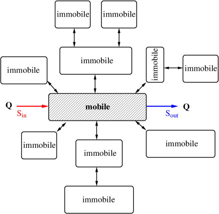
Figure 1: Example of a network with one mobile zone

We aim at describing the time evolution of the concentrations $S_{i}$ ($i=1\cdots n)$ of the solute in the $n$ tanks. The solute is injected in tank $1$ with a water flow rate $Q$ at a concentration $S_{in}$, and withdrawn from the same tank $1$ at the same water flow rate $Q$ with a concentration $S_{out}=S_{1}$. Thus, the tank $1$ plays the role of the mobile zone. We represent this system by a system of $n$ ordinary equations:

$$\begin{array}[]{rll}\dot{S}_{1}&=&\displaystyle\frac{Q}{V_{1}}(S_{in}-S_{1})+\sum_{j=2}^{n}\frac{d_{1j}}{V_{1}}(S_{j}-S_{1})\\ \vdots&&\vdots\\ \dot{S}_{i}&=&\displaystyle\sum_{j\neq i}\frac{d_{ij}}{V_{i}}(S_{j}-S_{i})\\ \vdots&&\vdots\\ \end{array}$$

where the parameters $d_{ij}=d_{ji}$ ($i\neq j)$ denote the diffusive exchange rates of solute between reservoirs $i$ and $j$. For sake of simplicity, we shall assume

$$\frac{Q}{V_{1}}=1$$

which is always possible by a change of the time scale of the dynamics. In the following we adopt an input-output setting in matrix form:

$$\begin{array}[]{lll}\dot{X}&=&AX+Bu\\ y&=&CX\end{array}$$ (1)

where $X$ denotes the vector of the concentrations $S_{i}$ ($i=1\cdots n$), $u$ the input that is $u=S_{in}$ and $y$ the output $y=S_{out}=S_{1}$. The column and row matrices $B$ and $C$ are as follows

$$B=\left[\begin{array}[]{c}1\\ 0\\ \vdots\\ 0\end{array}\right]\quad\mbox{and}\quad C=\left[\begin{array}[]{cccc}1&0&\dots&0\end{array}\right]\$$

and the matrix $A$ satisfies the following properties.

Assumptions 1.1.

There exist matrices $V$ and $M$ such that

$$A=-BB^{t}-V^{-1}M$$

where $V$ is a positive diagonal matrix and $M$ is a symmetric matrix that fulfills

1. $M$ is irreducible (i.e. the graph with nodes $P_{i}$, and edges $\overrightarrow{P_{i}P_{j}}$ when $M_{ij}\neq 0$ is strongly connected)

2. $M_{ii}>0$ for any $i$

3. $M_{ij}\leq 0$ for any $i\neq j$

4. $\sum_{j}M_{ij}=0$ for any $i$

The diagonal terms of the matrix $V$ represent the volumes of the $n$ zones, and the off diagonal terms $M_{i,j}$ of the matrix $M$ are the (opposite) of the diffusive exchange rate parameters between zones $i$ and $j$ (equal to $0$ if $i$ is not directly connected to $j$). Properties i. and iv. are related to the connectivity of the graph between zones and the mass conservation (i.e. Kirchoff’s law). One can proceed to the following reconstruction of matrices $V$ and $M$ from a given matrix $A$ that fulfills Assumptions 1.1.

Lemma 1.1.

Let $A$ fulfills Assumptions 1.1. For any $i=2\cdots n$, there exists a permutation $\pi$ of $\{1,\cdots,n\}$ and an integer $l<n$ such that $A_{\pi(j),\pi(j+1)}\neq 0$ $(j=1\cdots l)$ with $\pi(1)=1$ and $\pi(l+1)=i$. Define then the numbers

$$V_{\pi(j+1)}=V_{\pi(j)}\frac{A_{\pi(j+1)\pi(j)}}{A_{\pi(j)\pi(j+1)}}\quad j=1\cdots l$$ (2)

with $V_{1}=1$. Then $V$ is the diagonal matrix with $V_{1},\cdots,V_{n}$ as diagonal entries, and $M=-V(A+BB^{t})$.

Proof.

Under Assumptions 1.1, there exists for any $i\neq 1$ a path from node $1$ to $i$ in the direct graph associated to the matrix $A$, visiting nodes only once, for which one can associate a permutation $\pi$ such that $\pi(1)=1$, $\pi(l+1)=i$ with $A_{\pi(j)\pi(j+1)}\neq 0$ for $j=1\cdots l$, where $l<n$ is the path length. Furthermore, one has (by Assumptions 1.1)

$$\frac{A_{\pi(j)\pi(j+1)}}{V_{\pi(j)}}=\frac{A_{\pi(j+1)\pi(j)}}{V_{\pi(j+1)}},\quad j=1,\cdots,l.$$

One can then determine recursively the volumes $V_{\pi(1)}\cdots V_{\pi(l+1)}$ with the expression (2) from $V_{\pi(1)}=V_{1}$ that can be chosen equal to $1$. From the diagonal matrix $V$ whose diagonal entries are the (non-null) volumes $V_{1}\cdots V_{n}$, one can then reconstruct the matrix $M=-V(A+BB^{t})$. ∎

Matrices $A$ that fulfill Assumption 1.1 are compartmental matrices, that have been extensively studied in the literature (see for instance [20, 30]). In the present work, we focus on properties for the specific structure of compartmental matrices that we consider. We first define in Section 4 the two particular structures denoted MRMT and MINC, and give some of their properties. In Sections 5 and 6 we state and prove our main results about the equivalence of any network structure with these two particular structures, under Assumption 1.1 and an additional condition about the controllability. Section 7 discuss the crucial role played by this controllability assumption to obtain the equivalence. Finally, we draw conclusions with insights for geosciences.

2 Notations and preliminary results

For sake of simplicity, we introduce the following notations

• for any vector $X\in\mathbb{R}^{n}$ and matrix $Z\in{\cal M}_{n,n}(\mathbb{R})$, we denote

  $$\tilde{X}=[X_{i}]_{i=2\cdots n}\ ,\qquad\tilde{Z}=[Z_{ij}]\mathop{{}_{i=2\cdots n}}_{j=2\cdots n}\ .$$

• $\mbox{\em diag}\,(X)$ denotes the diagonal matrix whose diagonal elements are the entries of the vector $X$

• we denote by $\mbox{\em Vand}\,(x_{1},\cdots,x_{m})$ the (square) Vandermonde matrix

  $$\mbox{\em Vand}\,(x_{1},\cdots,x_{m})=\left[\begin{array}[]{llll}1&x_{1}&\cdots&x_{1}^{m-1}\\ \vdots&\vdots&\vdots&\vdots\\ 1&x_{m}&\cdots&x_{m}^{m-1}\end{array}\right]$$

• we define the vector in $\mathbb{R}^{n}$

  $$\mathbbm{1}=\left[\begin{array}[]{c}1\\ \vdots\\ 1\end{array}\right]\ .$$

Lemma 2.1.

Under Assumptions 1.1, the domain $\mathbb{R}_{+}^{n}$ is invariant by the dynamics for any non-negative control $u$.

Proof.

Take a vector $X$ that is on the boundary of $\mathbb{R}_{+}^{n}$ and set $I=\{i\in 1\cdots n\,|\,X_{i}=0\}$. At such a vector, one has

$$\dot{X}_{i}=\sum_{j\notin}A_{i,j}X_{j}+B_{i}u\ ,\quad i\in I$$

Notice that the matrix $A$ is Metzler (that is all its non-diagonal terms are non-negative) and $B$ is a non-negative vector. Consequently one has

$$\dot{X}_{i}\geq 0\ ,\quad i\in I$$

which proves that any forward trajectory cannot leave the non-negative cone. ∎

Remark 2.1.

Under Assumptions 1.1, the linear system (1) is positive in the sense that for any non-negative initial state and non negative control $u(\cdot)$, state and output are non-negative for any positive time (see [12]).

Lemma 2.2.

Under Assumptions 1.1, the matrix $\tilde{M}$ is symmetric definite positive.

Proof.

The matrix $\tilde{M}$ is symmetric and consequently it is diagonalizable with real eigenvalues. Its diagonal terms are positive and off-diagonal negative or equal to zero. Furthermore one as

$$\tilde{M}_{ii}=M_{i+1,i+1}=-\sum_{j\neq i+1}M_{i+1,j}=-\sum_{j\neq i}\tilde{M}_{i,j}-M_{i+1,1}\geq-\sum_{j\neq i}\tilde{M}_{i,j}$$

The matrix $\tilde{M}$ is thus (weakly) diagonally dominant. As each irreducible block of the matrix $\tilde{M}$ has to be connected to the mobile zone (otherwise the matrix $A$ won’t be irreducible), we deduce that at least one line of each block has to be strictly diagonally dominant. Then, each block is irreducibly diagonally dominant and thus invertible by Taussky Theorem (see [19, 6.2.27]). Finally, the eigenvalues of the matrix $\tilde{M}$ belong to the Gershgorin discs

$$G(\tilde{M})=\bigcup_{i}\left\{\lambda\in\mathbb{R}\,|\,|\lambda-\tilde{M}_{i,i}|\leq\sum_{j\neq i}|\tilde{M}_{i,j}|\right\}$$

and we deduce that each eigenvalues $\tilde{\lambda}_{i}$ of $\tilde{M}$ are positive. The matrix $\tilde{M}$ is thus symmetric definite positive. ∎

Lemma 2.3.

Under Assumptions 1.1, the matrix $A$ is non singular. Furthermore, the dynamics admits the unique equilibrium $\mathbbm{1}u$, for any constant control $u$

Proof.

Let $X$ be a vector such that $AX=0$. Then, one has $BB^{t}X=-V^{-1}MX$ or equivalently

$$MX=-V_{1}X_{1}B\ .$$

Let us decompose the matrix $M$ as follows

$$M=\left[\begin{array}[]{cc}M_{11}&L\\ L^{\prime}&\tilde{M}\end{array}\right]$$

where $L$ is a row vector of length $n-1$. Then equality $MX=-V_{1}X_{1}B$ amounts to write

$$\left\{\begin{array}[]{l}M_{11}X_{1}+L\tilde{X}=-V_{1}X_{1}\\ L^{\prime}X_{1}+\tilde{M}\tilde{X}=0\end{array}\right.$$

$\tilde{M}$ being invertible (Lemma 2.2), one can write $\tilde{X}=-\tilde{M}^{-1}L^{\prime}X_{1}$ and thus $X_{1}$ has to fulfill

$$(M_{11}-L\tilde{M}^{-1}L^{\prime})X_{1}=-V_{1}X_{1}$$

From Assumptions 1.1, one has $M\mathbbm{1}=0$ which gives

$$\left\{\begin{array}[]{l}M_{11}+L\tilde{\mathbbm{1}}=0\\ L^{\prime}+\tilde{M}\tilde{\mathbbm{1}}=0\end{array}\right.$$

that implies $M_{11}-L\tilde{M}^{-1}L^{\prime}=0$. We conclude that one should have $X_{1}=0$ and then $\tilde{X}=0$, that is $X=0$. The matrix $A$ is thus invertible.

Finally, the system admits an unique equilibrium $X^{\star}=-A^{-1}Bu$ for any constant control $u$. As Assumptions 1.1 imply the equality $A\mathbbm{1}=-B$, we deduce that the equilibrium is given by $X^{\star}=\mathbbm{1}u$.

∎

Lemma 2.4.

Under Assumptions 1.1, the sub-matrix $\tilde{A}$ is diagonalizable with real negative eigenvalues.

Proof.

Notice first that the matrix $\tilde{A}$ can be written as $\tilde{A}=-\tilde{V}^{-1}\tilde{M}$. The matrix $\tilde{V}$ being diagonal with positive diagonal terms, one can consider its square root $\tilde{V}^{1/2}$, defined as a diagonal matrix with $\sqrt{\tilde{V}_{i}}$ terms on the diagonal, and its inverse $\tilde{V}^{-1/2}$. Then, one has

$$\tilde{V}^{1/2}\tilde{A}\tilde{V}^{-1/2}=-\tilde{V}^{-1/2}\tilde{M}\tilde{V}^{-1/2}$$

which is symmetric. So $\tilde{A}$ is similar to a symmetric matrix, and thus diagonalizable. Let $\lambda$ be an eigenvalue of $\tilde{A}$. There exist an eigenvector $X\neq 0$ such that

$$\tilde{A}X=\lambda X\Rightarrow X^{\prime}\tilde{V}(\tilde{A}X)=\lambda X^{\prime}\tilde{V}X\Leftrightarrow X^{\prime}\tilde{M}X=-\lambda X^{\prime}\tilde{V}X$$

As $\tilde{M}$ is definite positive (Lemma 2.2) as well as $\tilde{V}$, we conclude that $\lambda$ has to be negative. ∎

3 About controllability and observability

We recall the usual definitions of controllability and observability of single-input single-output systems $(A,B,C)$ of dimension $n$ (see for instance [21]).

Definitions 3.1.

• The controllability matrix associated to the pair $(A,B)$ is given by

  $${\cal C}_{A,B}=[B,AB,\cdots,A^{n-1}B]$$

• The observability matrix associated to the pair $(A,C)$ is given by

  $${\cal O}_{A,C}=\left[\begin{array}[]{c}C\\ CA\\ \vdots\\ CA^{n-1}\end{array}\right]$$

• A system $\dot{X}=AX+Bu$ is said to be controllable when $\mbox{\em rk}\,({\cal C}_{A,B})=n$, and observable for $y=CX$ when $\mbox{\em rk}\,({\cal O}_{A,C})=n$.

• To a given triplet $(A,B,C)$, we associate the linear operator ${\cal F}_{A,B,C}:{\cal L}^{2}(\mathbb{R}_{+},\mathbb{R})\mapsto{\cal L}^{2}(\mathbb{R}_{+},\mathbb{R})$ that is defined as $y(\cdot)={\cal F}_{A,B,C}[u(\cdot)]$ with $y(\cdot)=CX(\cdot)$ where $X(\cdot)$ is solution of $\dot{X}=AX+Bu(\cdot)$ for the initial condition $X(0)=0$. We say that a triplet $(A,B,C)$ is a minimal representation if among all the triplets $(A^{\dagger},B^{\dagger},C^{\dagger})$ such that ${\cal F}_{A^{\dagger},B^{\dagger},C^{\dagger}}={\cal F}_{A,B,C}$, the dimension of $A$ is minimal.

We recall a well known result of the literature on linear input-output systems [21, 2.4.6].

Theorem 3.1.

(Kalman) A representation $(A,B,C)$ is minimal if and only if the pairs $(A,B)$ and $(A,C)$ are respectively controllable and observable.

The particular structures of the matrices $A$, $B$ and $C$ that we consider allow to show the following property.

Lemma 3.1.

Under Assumptions 1.1, $(A,B)$ controllable is equivalent to $(A,C)$ observable.

Proof.

Notice first that one has

$$VAV^{-1}=-BB^{t}-MV^{-1}=(-BB^{t}-V^{-1}M)^{\prime}=A^{\prime}$$

and by recursion

$$VA^{k}V^{-1}=(A^{\prime})^{k}$$

Then, one can write

$${\cal O}^{\prime}_{A,C}=[B,A^{\prime}B,(A^{\prime})^{2}B,\cdots]=V[V^{-1}B,AV^{-1}B,A^{2}V^{-1}B,\cdots]$$

But one has

$$V^{-1}B=V_{1}^{-1}B$$

Thus

$$V_{1}{\cal O}_{A,C}^{\prime}=V[B,AB,A^{2}B,\cdots]=V{\cal C}_{A,B}$$

and we conclude

$$\mbox{\em rk}\,({\cal O}_{A,C})=\mbox{\em rk}\,({\cal C}_{A,B}).$$

∎

We also recall a nice result about tridiagonalization of single-input single-output systems, from [16, Lemma 2.2].

Proposition 3.1.

Let $T$ be an invertible transformation, then one has

$$T^{-1}AT=\left[\begin{array}[]{ccccc}\star&y_{2}&&&\makebox(-10.0,-10.0)[]{\text{\em\Large 0}}\\ x_{2}&\ddots&\ddots&&\\ &\ddots&\ddots&\ddots&\\ &&\ddots&\ddots&y_{n}\\ \makebox(20.0,20.0)[]{\text{\em\Large 0}}&&&x_{n}&\star\end{array}\right],\quad T^{-1}B=\left[\begin{array}[]{c}x_{1}\\ 0\\ \vdots\\ \vdots\\ 0\end{array}\right],\quad CT=\left[\begin{array}[]{ccccc}y_{1}&0&\cdots&\cdots&0\end{array}\right]$$

with $x_{i}\neq 0$ and $y_{i}\neq 0$ $(i=1\cdot n)$ if and only if

$$T^{-1}{\cal C}_{A,B}=\left[\begin{array}[]{cccc}c_{1}&\star&\cdots&\star\\ &\ddots&\ddots&\vdots\\ &&\ddots&\star\\ \makebox(20.0,20.0)[]{\text{\em\Large 0}}&&&c_{n}\end{array}\right]\mbox{ and }{\cal O}_{A,C}T=\left[\begin{array}[]{cccc}o_{1}&&&\makebox(-10.0,-10.0)[]{\text{\em\Large 0}}\\ \star&\ddots&&\\ \vdots&\ddots&\ddots&\\ \star&\cdots&\star&o_{n}\end{array}\right]$$

with $c_{i}\neq 0$, $o_{i}\neq 0$ $(i=1\cdot n)$ . Furthermore, one has $x_{1}=c_{1}$, $y_{1}=o_{1}$, $x_{i+1}=c_{i+1}/c_{i}$, $y_{i+1}=o_{i+1}/o_{i}$ $(i=1\cdots n-1)$.

4 The Multi-Rate Mass Transfer and Multiple INteracting Continua configurations

We consider two particular structures of networks whose $(A,B,C)$ representations fulfill Assumption 1.1.

Definition 4.1.

A matrix $A$ that fulfills Assumptions 1.1 and such that the sub-matrix

$$\tilde{A}=[A_{ij}]\mathop{{}_{i=2\cdots n}}_{j=2\cdots n}$$

is diagonal is called a MRMT (multi-rate mass transfer) matrix.

MRMT matrices correspond to particular arrow structure of the matrix $A$:

$$A=\left[\begin{array}[]{cccccc}-\frac{Q}{V_{1}}-\sum_{i}\frac{d_{1i}}{V_{1}}&\frac{d_{12}}{V_{1}}&\cdots&\cdots&\cdots&\frac{d_{1n}}{V_{1}}\\[8.53581pt] \frac{d_{12}}{V_{2}}&-\frac{d_{12}}{V_{2}}&0&\cdots&\cdots&0\\[8.53581pt] \vdots&0&\ddots&\ddots&&\vdots\\[8.53581pt] \vdots&\vdots&&\ddots&\ddots&0\\[8.53581pt] \frac{d_{1n}}{V_{n}}&0&\cdots&\cdots&0&-\frac{d_{1n}}{V_{n}}\end{array}\right]$$

or star connections f the immobile part of depth one, where all the immobile zones are connected to the mobile one (see Fig. 2).

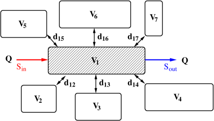
Figure 2: Example of a MRMT network

Definition 4.2.

A matrix $A$ that fulfills Assumptions 1.1 and which is tridiagonal is called a MINC (Multiple INteracting Continua) matrix.

MINC matrices correspond to particular structure:

$$A=\left[\begin{array}[]{rcccccc}\frac{Q}{V_{1}}-\frac{d_{12}}{V_{1}}&\frac{d_{12}}{V_{1}}&&&&\\[8.53581pt] \frac{d_{12}}{V_{2}}&-\frac{d_{12}+d_{23}}{V_{2}}&\frac{d_{23}}{V_{2}}&&&\makebox(0.0,0.0)[]{\text{\huge 0}}\\[8.53581pt] &\ddots&\ddots&\ddots&&&\\[8.53581pt] \makebox(0.0,0.0)[]{\text{\huge 0}}&&\ddots&\ddots&\ddots&&\\[8.53581pt] &&&&\frac{d_{n-1,n}}{V_{n}}&-\frac{d_{n-1,n}}{V_{n}}\end{array}\right]$$

where the immobile parts are connected in series, of length $n-1$, one of them being connected to the mobile zone (see Fig. 3).

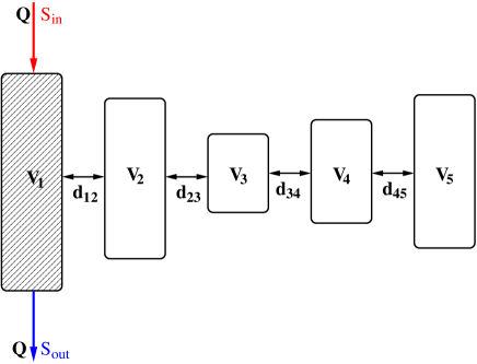
Figure 3: Example of a MINC network

In the following, we give properties on eigenvalues for MRMT matrices only, because it is easier to be proved for this particular structure. In the next section, we shall show that MINC and MRMT structures are indeed equivalent, and as a consequence eigenvalues of MINC matrices fulfill the same properties.

Lemma 4.1.

A MRMT matrix is Hurwitz (i.e. all the real parts of its eigenvalues are negative).

Proof.

Take a number

$$\gamma>\max\left(\frac{Q}{V_{1}}+\sum_{i}\frac{d_{1i}}{V_{1}},\frac{d_{12}}{V_{2}},\cdots,\frac{d_{1n}}{V_{n}}\right)\ .$$

Then the matrix $\gamma I+A$ is an irreducible non-negative matrix. From Perron-Frobenius Theorem (see [6, Th 1.4]), $r=\rho(\gamma I+A)$ is a single eigenvalue of $\gamma I+A$ and there exists a positive eigenvector associated to this eigenvalue. That amounts to claim that there exists a positive eigenvector $X$ of the matrix $A$ for a single (real) eigenvalue $\lambda=r-\gamma$, and furthermore that any other eigenvalue $\mu$ of $A$ is such that

$$-r<\gamma+\mbox{\em Re}\,(\mu)<r\;\Rightarrow\;\mbox{\em Re}\,(\mu)<\lambda\ .$$

From the particular structure of MRMT matrix, such a vector $X$ has to fulfill the equalities

$$\begin{array}[]{cll}\displaystyle-\frac{Q}{V_{1}}+\sum_{i=2}^{n}\frac{d_{1i}}{V_{1}}(X_{i}-X_{1})&=&\lambda X_{1}\\[11.38109pt] d_{1i}(X_{1}-X_{i})&=&\lambda V_{i}X_{i}\qquad(i=2\cdots n)\end{array}$$

from which one obtains

$$-\frac{Q}{V_{1}}=\lambda\left(X_{1}+\sum_{i=2}^{n}\frac{V_{i}}{V_{1}}X_{i}\right)\ .$$

The vector $X$ being positive, we deduce that $\lambda$ is negative. ∎

As $\mathbbm{1}u$ is an equilibrium of the system (1) for any constant control $u$, this Lemma allows then to claim the following result.

Lemma 4.2.

For any constant control $u$, $\mathbbm{1}u$ is a globally exponentially stable of the dynamics (1).

Finally, we characterize the minimal MRMT representations as follows.

Lemma 4.3.

For a minimal representation $(A,B,C)$ where $A$ is MRMT, the eigenvalues of the matrix $\tilde{A}$ are distinct.

Proof.

The eigenvalues of $\tilde{A}$ for the MRMT structure are $\lambda_{i}=-d_{1i}/V_{i}$ ($i=2\cdots n$). If there exist $i\neq j$ in $\{2,\cdots,n\}$ such that $\lambda_{i}=\lambda_{j}=\lambda$, one can consider the variable

$$S_{ij}=\frac{V_{i}}{V_{i}+V_{j}}S_{i}+\frac{V_{j}}{V_{i}+V_{j}}S_{j}$$

instead of $S_{i},S_{j}$ and write equivalently the dynamics in dimension $n-1$:

$$\begin{array}[]{rll}\dot{S}_{1}&=&\displaystyle\frac{Q}{V_{1}}(S_{in}-S_{1})+\sum_{k\geq 2,k\neq i,j}\frac{d_{1k}}{V_{1}}(S_{k}-S_{1})+\frac{d_{1ij}}{V_{ij}}(S_{ij}-S_{1})\\ \vdots&&\vdots\\ \dot{S}_{k}&=&\displaystyle\frac{d_{1k}}{V_{k}}(S_{1}-S_{k})\qquad k\in\{2,\cdots,n\}\setminus\{i,j\}\\ \vdots&&\vdots\\ \dot{S}_{ij}&=&\displaystyle\frac{d_{1ij}}{V_{ij}}(S_{1}-S_{ij})\\ \end{array}$$

with $V_{ij}=V_{i}+V_{j}$ and $d_{1ij}=-(V_{i}+V_{j})\lambda$, which show that $(A,B,C)$ is not minimal. ∎

In the coming sections, we address the equivalence problem of any network structure that fulfill Assumption 1.1 with either a MRMT or a MINC structure. There are many known ways to diagonalize the sub-matrix $\tilde{A}$ or tridiagonalize the whole matrix $A$ to obtain matrices similar to $A$ with an arrow or tridiagonal structure. The remarkable feature we prove is that there exist such transformations that preserve the signs of the entries of the matrices (i.e. Assumption 1.1 is also fulfilled in the new coordinates) so that the equivalent networks have a physical interpretation.

For a system $(A,B,C)$ that fulfills Assumption 1.1, we adress in the two coming Sections the problem of finding equivalent MRMT or MINC structure (which are two other positive realizations [5, 25, 4] of the input-output system).

5 Equivalence with MRMT structure

We first give sufficient conditions to obtain the equivalence with MRMT.

Proposition 5.1.

Under Assumption 1.1, take an invertible matrix $P$ such that $P^{-1}\tilde{A}P=\Delta$, where $\Delta$ is diagonal. If all the entries of the vector $P^{-1}\tilde{\mathbbm{1}}$ are non-null and the eigenvalues of $\tilde{A}$ are distinct, the matrix

$$R=\left[\begin{array}[]{cc}1&0\\ 0&-P\Delta^{-1}\mbox{\em diag}\,(P^{-1}A(2:n,1))\end{array}\right]$$

is invertible and such that $R^{-1}\!AR$ is a MRMT matrix.

Proof.

Take a general matrix $A$ that fulfills Assumption 1.1. From Lemma 2.4, $\tilde{A}$ is diagonalizable with $P$ such that $P^{-1}\tilde{A}P=\Delta$ where $\Delta$ is a diagonal matrix. Let $G$ be the diagonal matrix

$$G=-\Delta^{-1}\mbox{\em diag}\,(P^{-1}A(2:n,1))$$

and define $\tilde{R}=PG$.
Notice that one has $A\mathbbm{1}=-B$ from Assumptions 1.1. The $n-1$ lines of this equality gives $A(2:n,1)+\tilde{A}\tilde{\mathbbm{1}}=0$ and one can write

$$\begin{array}[]{ll}&P^{-1}A(2:n,1)+P^{-1}\tilde{A}\tilde{\mathbbm{1}}=0\\ \Leftrightarrow&P^{-1}A(2:n,1)+P^{-1}\tilde{A}PP^{-1}\tilde{\mathbbm{1}}=0\\ \Leftrightarrow&P^{-1}A(2:n,1)+\Delta P^{-1}\tilde{\mathbbm{1}}=0\end{array}$$

Thus having all the entries of the vector $P^{-1}A(2:n,1)$ non-null is equivalent to have all the entries of the vector $P^{-1}\tilde{\mathbbm{1}}$ non null.

All the entries of the vector $P^{-1}A(2:n,1)$ being non-null, $\tilde{R}$ is invertible and one has

$$\tilde{R}^{-1}\tilde{A}\tilde{R}=G^{-1}P^{-1}\tilde{A}PG=G^{-1}\Delta G=\Delta.$$

One can then consider the matrix $R\in{\cal M}_{n,n}$ defined as

$$R=\left[\begin{array}[]{cc}1&0\\ 0&\tilde{R}\end{array}\right]\quad\mbox{with}\quad R^{-1}=\left[\begin{array}[]{cc}1&0\\ 0&\tilde{R}^{-1}\end{array}\right]$$

One has

$$R^{-1}AR=\left[\begin{array}[]{cc}A_{11}&A(1,2:n)\tilde{R}\\[11.38109pt] \tilde{R}^{-1}A(2:n,1)&\Delta\end{array}\right]$$

We show now that the matrix $R^{-1}\!AR$ fulfills Assumptions 1.1.

One has straightforwardly

$$R^{-1}AR=-B^{t}B-R^{-1}V^{-1}MR\ .$$

As the irreducibility of the matrix $V^{-1}M$ is preserved by the change of coordinates given by $X\mapsto R^{-1}X$, Property i. is fulfilled.

The diagonal terms of $-(R^{-1}AR+BB^{t})$ are $-A_{11}-1$ (which is positive) and the diagonal of $-\Delta$ which is also positive. Property ii. is thus satisfied.

We have now to prove that column $\tilde{R}^{-1}A(2:n,1)$ and row $A(1,2:n)\tilde{R}$ are positive to show Property iii. From the definition of the matrix $G$, one has

$$\Delta=-G^{-1}\mbox{\em diag}\,(P^{-1}A(2:n,1))=-\mbox{\em diag}\,(\tilde{R}^{-1}A(2:n,1))$$

and thus one has

$$\tilde{R}^{-1}A(2:n,1)=-\Delta\tilde{\mathbbm{1}}$$

As the diagonal terms of $\Delta$ are negative, we deduce that the vector $\tilde{R}^{-1}A(2:n,1)$ is positive. As the matrix $V\!A$ is symmetric, one can write $V_{11}A(1,2:n)=A(2:n,1)^{\prime}\tilde{V}$ and then

$$\left(V_{11}A(1,2:n)\tilde{R}\right)^{\prime}=\tilde{R}^{\prime}\tilde{V}A(2:n,1)=-\tilde{R}^{\prime}\tilde{V}\tilde{R}\Delta\tilde{\mathbbm{1}}$$

Notice that the matrix $\tilde{R}^{\prime}\tilde{V}\tilde{R}$ can be written $T^{\prime}T$ with $T=\tilde{V}^{1/2}\tilde{R}$, and that the matrix $T$ diagonalizes the matrix $S=\tilde{V}^{1/2}\tilde{A}\tilde{V}^{-1/2}$:

$$T^{-1}ST=\tilde{R}^{-1}\tilde{A}\tilde{R}=\Delta$$

The matrix $S$ being symmetric, it is also diagonalizable with a unitary matrix $U$ such that $U^{\prime}SU=\Delta$. As the eigenvalues of $\tilde{A}$ are distinct, their eigenspaces are one-dimensional and consequently the columns of any matrix that diagonalizes $S$ into $\Delta$ have to be proportional to corresponding eigenvectors. So the matrix $T$ is of the form $UD$ where $D$ is a non-singular diagonal matrix. This implies that the matrix $\tilde{R}^{\prime}\tilde{V}\tilde{R}$ is equal to $D^{2}$, which is a positive diagonal matrix. As $-\Delta\tilde{\mathbbm{1}}$ is a positive vector, we deduce that the entries of $A(1,2:n)\tilde{R}$ are positive.

Notice that $\tilde{\mathbbm{1}}$ is necessarily an eigenvector of $\tilde{R}^{-1}$ (or $\tilde{R}$) for the eigenvalue $1$: as one has $A\mathbbm{1}=-B$, one has also $A(2:n,1)=-\tilde{A}\tilde{\mathbbm{1}}$ and then

$$\tilde{R}^{-1}\tilde{\mathbbm{1}}=-\tilde{R}^{-1}\tilde{A}^{-1}A(2:n,1)=-\Delta^{-1}\tilde{R}^{-1}A(2:n,1)=-\Delta^{-1}\mbox{\em diag}\,(\tilde{R}^{-1}A(2:n,1))\tilde{\mathbbm{1}}=\tilde{\mathbbm{1}}$$

Finally, one has

$$(R^{-1}AR+BB^{t})\mathbbm{1}=R^{-1}A\mathbbm{1}+B=-R^{-1}B+B=0$$

which proves that Property iv. is verified.

∎

We come back to the condition required by Proposition 5.1 and show that it is necessarily fulfilled for minimal representations (we recall from Lemma 3.1 that controllability implies a minimal representation in our framework).

Proposition 5.2.

Under Assumptions 1.1, the entries of the vector $P^{-1}\tilde{\mathbbm{1}}$ are non null for any $P$ such that $P^{-1}\tilde{A}P=\Delta$ with $\Delta$ diagonal, when the pair $(A,B)$ is controllable. Furthermore, the eigenvalues of $\tilde{A}$ are distinct.

Proof.

From Lemma 2.4, $\tilde{A}$ is diagonalizable with $P$ such that $P^{-1}\tilde{A}P=\Delta$ where $\Delta$ is a diagonal matrix. Posit $X=P^{-1}\tilde{\mathbbm{1}}$. One has

$$P^{-1}\tilde{A}^{k}P=\Delta^{k}\;\Longrightarrow\;P^{-1}\tilde{A}^{k}\tilde{\mathbbm{1}}=\Delta^{k}X\ ,\quad k=1,\cdots$$

This implies

$$P^{-1}\left[\tilde{\mathbbm{1}},\tilde{A}\tilde{\mathbbm{1}},\cdots,\tilde{A}^{n-1}\tilde{\mathbbm{1}}\right]=\mbox{\em diag}\,(X)Vand(\lambda_{1},\cdots,\lambda_{n})$$

or equivalently

$$P^{-1}{\cal C}_{\tilde{A},\tilde{\mathbbm{1}}}=\mbox{\em diag}\,(X)Vand(\lambda_{1},\cdots,\lambda_{n-1})$$

We deduce that when ${\cal C}_{\tilde{A},\tilde{\mathbbm{1}}}$ is full rank, $\mbox{\em diag}\,(X)$ and $Vand(\lambda_{1},\cdots,\lambda_{n-1})$ are non-singular, that is all the entries of $X$ are non-null and the eigenvalues $\lambda_{1},\cdots,\lambda_{n-1}$ are distinct. We show now that the controllability of the pair $(A,B)$ implies that the pair $(\tilde{A},\tilde{\mathbbm{1}})$ is also controllable.

From the property $A\mathbbm{1}=-B$, one can write

$$A=\left[\begin{array}[]{rl}A_{11}&L\\ -\tilde{A}\tilde{\mathbbm{1}}&\tilde{A}\end{array}\right]$$

where $L$ is a row vector of length $n-1$. Then one has

$$A\mathbbm{1}=\left[\begin{array}[]{c}-1\\ \tilde{0}\end{array}\right]\ ,\quad A^{2}\mathbbm{1}=\left[\begin{array}[]{c}-A_{11}\\ \tilde{A}\tilde{\mathbbm{1}}\end{array}\right]\ ,\quad A^{3}\mathbbm{1}=\left[\begin{array}[]{c}-A_{11}^{2}+L\tilde{A}\tilde{\mathbbm{1}}\\ A_{11}\tilde{A}\tilde{\mathbbm{1}}+\tilde{A}^{2}\mathbbm{1}\end{array}\right]$$

that are of the form

$$A^{k}\mathbbm{1}=\left[\begin{array}[]{c}\alpha_{k}\\ P_{k}\end{array}\right]\mbox{ with }P_{k}=\tilde{A}^{k-1}\mathbbm{1}+\displaystyle\sum_{j\leq k-2}\beta_{kj}\tilde{A}^{j}\mathbbm{1}\ ,\mbox{ for }k=2,3$$

By recursion, one obtains

$$P_{k+1}=-\alpha_{k}\tilde{A}\tilde{\mathbbm{1}}+\tilde{A}^{k}\mathbbm{1}+\displaystyle\sum_{j\leq k-2}\beta_{kj}\tilde{A}^{j+1}\mathbbm{1}=\tilde{A}^{k}\mathbbm{1}+\displaystyle\sum_{j\leq k-1}\beta_{k+1,j}\tilde{A}^{j}\mathbbm{1}\ ,\mbox{ for }k=2,\cdots$$

Then, one can write

$$-{\cal C}_{A,B}={\cal C}_{A,A\mathbbm{1}}=\left[\begin{array}[]{llll}\alpha_{1}&\alpha_{2}&\cdots&\alpha_{n}\\ \tilde{0}&P_{2}&\cdots&P_{n}\end{array}\right]$$

from which one deduces

$$\mbox{\em rk}\,({\cal C}_{A,B})=n\;\Rightarrow\;\mbox{\em rk}\,(P_{2},\cdots,P_{n})=n-1\;\Rightarrow\;\mbox{\em rk}\,(\tilde{A}\mathbbm{1},\cdots\tilde{A}^{n-1}\mathbbm{1})=n-1$$

One can also write $[\tilde{A}\mathbbm{1},\cdots\tilde{A}^{n-1}\mathbbm{1}]=\tilde{A}{\cal C}_{\tilde{A},\tilde{\mathbbm{1}}}$ and as $\tilde{A}$ is invertible (Lemma 2.4), we finally obtain that ${\cal C}_{\tilde{A},\tilde{\mathbbm{1}}}$ is full rank. ∎

Finally, Propositions 5.1 and 5.2 lead to the main result of this section.

Theorem 5.1.

Any minimal representation $(A,B,C)$ that fulfills Assumptions 1.1 is equivalent to a MRMT structure.

6 Equivalence with MINC structure

Take a matrix $A$ that fulfills Assumption 1.1 and such that that pair $(A,B)$ is controllable. As we have already shown that such representation $(A,B,C)$ is minimal and equivalent to a MRMT configuration, we can assume without any loss of generality that the matrix $A$ has the structure

$$A=\left[\begin{array}[]{cc}A_{11}&A(1,2:n)\\[5.69054pt] A(2:n,1)&\Delta\end{array}\right]$$

where $\Delta$ is a square diagonal matrix (of size $n-1$) with distinct negative eigenvalues. We denote by $V$ the diagonal matrix of the volumes associated to the matrix $A$ with $V_{1}=1$, as given by Lemma 1.1 We shall consider a tridiagonalization of this matrix. For this purpose, we recall the Lanczos algorithm.

Definition 6.1.

(Lanczos algorithm) Let $S$ be a symmetric matrix of size $m$ and $q_{1}$ be a vector of norm equal to one. One defines the sequence $\pi_{k}=(\beta_{k},q_{k},r_{k})$ as follows

• $\beta_{0}=0$, $q_{0}=0$, $r_{0}=q_{1}$,

• if $\beta_{k}\neq 0$, define $q_{k+1}=r_{k}/\beta_{k}$, $\alpha_{k+1}=q_{k+1}^{\prime}Sq_{k+1}$, $r_{k+1}=(S-\alpha_{k+1}I)q_{k+1}-\beta_{k}q_{k}$ and $\beta_{k+1}=||r_{k+1}||$.

One can straightforwardly check that the vectors $q_{k}$ provided by this algorithm are orthogonal and of norm equal to one. The algorithm stops for $k<m$ (“breakdown”) or $k=m$. A non-breakdown condition for this algorithm is given in [17, Th 10.1.1]:

Proposition 6.1.

When $\mbox{\em rk}\,({\cal C}_{S,q_{1}})=m$, the sequence $\pi_{k}$ is defined up to $k=m$, and the matrix $Q=[q_{1}\cdots q_{m}]$ verifies

$$Q^{\prime}AQ=\left[\begin{array}[]{ccccc}\alpha_{1}&\beta_{1}&&&\makebox(-10.0,-10.0)[]{\text{\em\Large 0}}\\ \beta_{1}&\ddots&\ddots&&\\ &\ddots&\ddots&\ddots&\\ &&\ddots&\ddots&\beta_{m-1}\\ \makebox(20.0,20.0)[]{\text{\em\Large 0}}&&&\beta_{m-1}&\alpha_{m}\end{array}\right]$$

where the numbers $\beta_{i}$ $(i=1\cdots m)$ are positive.

Lemma 6.1.

The Lanczos algorithm applied to the matrix $\Delta$ with $q_{1}=A(2:n,1)/||A(2:n,1)||$ provides an orthogonal unitary matrix $Q$ such that $Q^{\prime}\Delta Q$ is symmetric tridiagonal with positive terms on the sub- (or super-) diagonal.

Proof.

As the matrix $\Delta$ is diagonal, one has

$${\cal C}_{\Delta,q_{1}}=\mbox{\em Vand}\,(\lambda_{1},\cdots,\lambda_{n-1})\mbox{\em diag}\,(q_{1})$$

where $\lambda_{i}$ $(i=1\cdots n-1)$ are the diagonal elements of $\Delta$. Furthermore, as Assumptions 1.1 imply the equality $A\mathbbm{1}=-B$, one has

$$q_{1}=-\frac{1}{\sqrt{\sum_{i=1}^{n-1}\lambda_{i}}}\left[\begin{array}[]{c}\lambda_{1}\\ \vdots\\ \lambda_{n-1}\end{array}\right]$$

As $\lambda_{i}$ are all distinct and non null, $q_{1}$ is a non null vector and the matrices $\mbox{\em Vand}\,(\lambda_{1},\cdots,\lambda_{n-1})$, $\mbox{\em diag}\,(q_{1})$ are full rank. Therefore ${\cal C}_{\Delta,q_{1}}$ is full rank and Proposition 6.1 can be used. ∎

Let us recall the well known Cholesky decomposition of symmetric matrix.

Theorem 6.1.

Let $S$ be a symmetric definite positive matrix. Then, there exists an unique upper triangular matrix $U$ with positive diagonal entries such that $S=U^{\prime}U$.

We are ready now to explicit a tridiagonalization of the matrix $A$ with positive entries on the sub- and super-diagonals.

Proposition 6.2.

Let $A$ be a MRMT matrix such that $(A,B)$ is controllable. Let $Q$ be the orthogonal matrix given by the Lanczos algorithm applied to $\Delta$ with $q_{1}=A(2:n,1)/||A(2:n,1)||$. Let $U$ be the upper triangular matrix with positive diagonal entries given by the Cholesky decomposition of the symmetric matrix $Q^{\prime}\tilde{V}Q$. Then the matrix

$$T=\left[\begin{array}[]{cc}1&0\\ 0&QU^{-1}\end{array}\right]$$

is such that $T^{-1}AT$ is symmetric tridiagonal with positive entries on the sub- (or super-)diagonal.

Proof.

Lemma 6.1 provides the existence of the matrix $Q$ such that $Q^{\prime}\Delta Q$ is tridiagonal with positive terms on the sub- and super-diagonal. For convenience, we define the matrices

$$P=\left[\begin{array}[]{cc}1&0\\ 0&Q\end{array}\right]\quad\mbox{and}\quad W=\left[\begin{array}[]{cc}1&0\\ 0&U\end{array}\right].$$

Clearly, $P$ is orthogonal, $W$ is upper triangular with positive diagonal, and one has $T=PW^{-1}$. Consider the matrix

$$P^{\prime}AP=\left[\begin{array}[]{cc}A_{11}&A(1,2:n)Q\\[5.69054pt] Q^{\prime}A(2:n,1)&Q^{\prime}\Delta Q\end{array}\right].$$

For the particular choice of the first column of $Q$, one has

$$Q^{\prime}A(2:n,1)=\frac{1}{||A(2:n,1)||}\left[\begin{array}[]{c}1\\ 0\\ \vdots\\ 0\end{array}\right]$$

and $Q^{\prime}\Delta Q$ is triangular with positive sub-diagonal. Therefore, $P^{\prime}AP$ is an upper Hessenberg matrix with positive entries on its sub-diagonal. Consider then

$$\begin{array}[]{lll}P^{\prime}{\cal C}_{A,B}&=&P^{\prime}\left[\begin{array}[]{cccc}B&AB&A^{2}B&\cdots\end{array}\right]\\[5.69054pt] &=&\left[\begin{array}[]{cccc}P^{\prime}B&(P^{\prime}AP)P^{\prime}B&(P^{\prime}A^{2}P)P^{\prime}B&\cdots\end{array}\right]\end{array}$$

Notice that one has $P^{\prime}B=B$ and obtains recursively

$$P^{\prime}B=\left[\begin{array}[]{c}h_{1}\\ 0\\ \vdots\\ \vdots\\ 0\end{array}\right],\quad(P^{\prime}AP)B=\left[\begin{array}[]{c}\star\\ h_{2}\\ 0\\ \vdots\\ \vdots\\ 0\end{array}\right],\quad(P^{\prime}A^{2}P)B=\left[\begin{array}[]{c}\star\\ \star\\ h_{3}\\ 0\\ \vdots\\ 0\end{array}\right],\quad\cdots$$

where the number $h_{i}$ are positive. Therefore, the matrix $P^{\prime}{\cal C}_{A,B}$ is upper triangular with positive diagonal, as the matrix $W$. Then $T^{-1}{\cal C}_{A,B}=WP^{\prime}{\cal C}_{A,B}$ is also upper triangular with positive entries on its diagonal. Proposition 3.1 implies that $T^{-1}AT$ is tridiagonal with positive entries on its sub-diagonal. Let us show that $T^{-1}AT$ is also symmetric. One has

$$T^{-1}AT=\left[\begin{array}[]{cc}A_{11}&A(1,2:n)QU^{-1}\\[5.69054pt] UQ^{\prime}A(2:n,1)&UQ^{\prime}\Delta QU^{-1}\end{array}\right]$$

As the matrix $VA$ is symmetric by Assumption 1.1, one can write

$$\begin{array}[]{lll}\left(A(1,2:n)QU^{-1}\right)^{\prime}&=&\frac{1}{V_{1}}(U^{-1})^{\prime}Q^{\prime}\tilde{V}A(2:n,1)\\ &=&\frac{1}{V_{1}}(U^{-1})^{\prime}U^{\prime}UQ^{\prime}A(2:n,1)\\ &=&\frac{1}{V_{1}}UQ^{\prime}A(2:n,1)\end{array}$$

and as we have chosen $V_{1}=1$ we obtain $\left(A(1,2:n)QU^{-1}\right)^{\prime}=UQ^{\prime}A(2:n,1)$. Consider now the sub-matrix $UQ^{\prime}\Delta QU^{-1}$. Notice first that the decomposition $Q^{\prime}\tilde{V}Q=U^{\prime}U$ implies the equalities $U^{\prime}=Q^{\prime}\tilde{V}QU^{-1}$ and $(U^{-1})^{\prime}=UQ^{\prime}\tilde{V}^{-1}Q$. Then on can write

$$\begin{array}[]{ccc}\left(UQ^{\prime}\Delta QU^{-1}\right)^{\prime}&=&(U^{-1})^{\prime}Q^{\prime}\Delta QU^{\prime}\\ &=&(UQ^{\prime}\tilde{V}^{-1}Q)Q^{\prime}\Delta Q(Q^{\prime}\tilde{V}QU^{-1})\\ &=&UQ^{\prime}\tilde{V}^{-1}\Delta\tilde{V}QU^{-1}\\ &=&UQ^{\prime}\Delta QU^{-1}\end{array}$$

∎

The matrix $T$ provided by Proposition 6.2 possesses the following property.

Proposition 6.3.

The vector $X=T^{-1}\mathbbm{1}$, where the matrix $T$ is provided by Proposition 6.2, is positive.

Proof.

The matrices $A+BB^{\prime}$ and $T^{-1}AT+BB^{\prime}$ have non-negative entries outside their main diagonals. So there exists a number $\gamma>0$ such that $I+\frac{1}{\gamma}(A+BB^{\prime})$ and $I+\frac{1}{\gamma}(T^{-1}AT+BB^{\prime})$ are non-negative matrices.

By Assumption 1.1, one has $A\mathbbm{1}=-B$, which implies the property

$$\left(I+\frac{1}{\gamma}(A+BB^{\prime})\right)\mathbbm{1}=\mathbbm{1}\ .$$

Thus $I+\frac{1}{\gamma}(A+BB^{\prime})$ is a stochastic matrix, and we know that its maximal eigenvalue is $1$ (see for instance [6, Th 5.3]). As $I+\frac{1}{\gamma}(A+BB^{\prime})$ and $I+\frac{1}{\gamma}(T^{-1}AT+BB^{\prime})$ are similar:

$$T^{-1}\left(I+\frac{1}{\gamma}(T^{-1}AT+BB^{\prime})\right)T=I+\frac{1}{\gamma}(A+BB^{\prime}),$$

the maximal eigenvalue of $I+\frac{1}{\gamma}(T^{-1}AT+BB^{\prime})$ is also $1$. Furthermore, as $A+BB^{\prime}$ is irreducible by Assumption 1.1, $I+\frac{1}{\gamma}(T^{-1}AT+BB^{\prime})$ is also irreducible. The property $A\mathbbm{1}=-B$ implies

$$\left(I+\frac{1}{\gamma}(T^{-1}AT+BB^{\prime})\right)X=X+\frac{1}{\gamma}(T^{-1}A\mathbbm{1}+B)=X+\frac{1}{\gamma}(-T^{-1}B+B)=X.$$

So $X$ is an eigenvector of $I+\frac{1}{\gamma}(T^{-1}AT+BB^{\prime})$ for its maximal eigenvalue $1$. Finally, notice that $X=T^{-1}\mathbbm{1}$ implies that the first entry of $X$ is equal to $1$. Then, by Perron-Frobenius Theorem (for non-negative irreducible matrices, see for instance [6, Th 1.4])), we conclude that $X$ is a positive vector. ∎

We give now our main result concerning the MINC equivalence.

Proposition 6.4.

Let $A$ be a MRMT matrix such that $(A,B)$ is controllable and $R=T\mbox{\em diag}\,(T^{-1}\mathbbm{1})$, where $T$ is provided by Proposition 6.2. Then $(R^{-1}AR,B,C)$ is an equivalent representation where $R^{-1}AR$ is a MINC matrix.

Proof.

Let $X=T^{-1}\mathbbm{1}$ and $\bar{A}=R^{-1}AR$. Define $\bar{V}=\mbox{\em diag}\,(X)^{2}$ and $\bar{M}=-\bar{V}(\bar{A}+BB^{\prime})$. As $A+BB^{\prime}$ is irreducible by Assumption 1.1, the similar matrix $\bar{A}+BB^{\prime}$ is also irreducible, as well as $\bar{M}$ because $V$ is a diagonal invertible matrix.

By Proposition 6.2, $T^{-1}AT$ is a symmetric tridiagonal matrix with positive terms on the sub- or super-diagonal. By Proposition 6.3, $X$ is a positive vector, and thus $\bar{A}=\mbox{\em diag}\,(X)^{-1}(T^{-1}AT)\mbox{\em diag}\,(X)$ is also a tridiagonal matrix with the same signs outside the diagonal. Thus, $\bar{M}$ is a tridiagonal matrix with negative terms on sub- or super-diagonal. Moreover, one has

$$\bar{M}=-\mbox{\em diag}\,(X)^{2}(\mbox{\em diag}\,(X)^{-1}T^{-1}AT\mbox{\em diag}\,(X)+BB^{\prime})=-\mbox{\em diag}\,(X)T^{-1}AT\mbox{\em diag}\,(X)-X_{1}^{2}.BB^{\prime}.$$

where $X_{1}=1$. The matrix $\bar{M}$ is thus symmetric. One has

$$\begin{array}[]{lll}\bar{M}\mathbbm{1}&=&-\mbox{\em diag}\,(X)T^{-1}AT\mbox{\em diag}\,(X)\mathbbm{1}-BB^{\prime}\mathbbm{1}\\ &=&-\mbox{\em diag}\,(X)T^{-1}ATX-B\\ &=&-\mbox{\em diag}\,(X)T^{-1}AT(T^{-1}\mathbbm{1})-B\\ &=&-\mbox{\em diag}\,(X)T^{-1}A\mathbbm{1}-B\\ &=&\mbox{\em diag}\,(X)T^{-1}B-B\\ &=&\mbox{\em diag}\,(X)B-B\\ &=&0\end{array}$$

The matrix $\bar{M}$ thus fulfills Assumption 1.1 and is tridiagonal: $\bar{A}$ is then a MINC matrix. Finally, one has $\bar{B}=R^{-1}B=B$ and $\bar{C}=CR=C$. ∎

Finally, Theorem 5.1 and Proposition 6.4 lead to the following result.

Theorem 6.2.

Any minimal representation $(A,B,C)$ that fulfills Assumptions 1.1 is equivalent to a MINC structure.

7 Examples and discussion

Theorems 5.1 and 6.2 show that whatever is the network structure, it is always possible to represent its input-output map with either a MRMT star or a MINC series structure. But from a state-space representation (1), it requires the system to be controllable (or minimal). We begin by an example that illustrates the necessity of the controllability assumption to make the equivalence constructions given in Sections 5, 6 work.

7.1 Example 1

Consider a network of four reservoirs of volumes (see Fig. 4)

$$V_{1}=1\ ,\;V_{2}=1\ ,\;V_{3}=2\ ,\;V_{4}=3$$

with the diffusive exchange rate coefficients:

$$d_{12}=1\ ,\;d_{13}=2\ ,\;d_{14}=3\ ,\;d_{23}=3\ ,\;d_{24}=3$$

which lead to the dynamics

$$\begin{array}[]{lll}\dot{S}_{1}&=&-7S_{1}+S_{2}+2S_{3}+3S_{4}+u\\ \dot{S}_{2}&=&S_{1}-7S_{2}+3S_{3}+3S_{4}\\ \dot{S}_{3}&=&S_{1}+\frac{3}{2}S_{2}-\frac{5}{2}S_{3}\\ \dot{S}_{4}&=&S_{1}+S_{2}-2S_{4}\end{array}$$

with the matrix

$$A=\left[\begin{array}[]{rrrr}-7&1&2&3\\ 1&-7&3&3\\ 1&\frac{3}{2}&-\frac{5}{2}&0\\ 1&1&0&-2\end{array}\right]$$

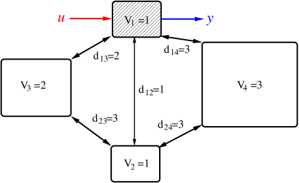
Figure 4: Structure of the example

At the first look, this structure does not exhibit any special property or symmetry that could make believe that it is non minimal. By construction one has $\tilde{A}\tilde{\mathbbm{1}}=-\tilde{\mathbbm{1}}$ but the particular matrix $A$ that we consider satisfies $A(2:4,1)=\tilde{\mathbbm{1}}$. Consequently the vector $A(2:4,1)$ is an eigenvector of the matrix $\tilde{A}$ for the eigenvalue $-1$. If the multiplicity of $-1$ was more than $1$, then $\lambda=-9.5$ should be an eigenvalue of $\tilde{A}$, as the trace of $\tilde{A}$ is $-11.5$. But an eigenvector $X$ of $\tilde{A}$ fulfills

$$\begin{array}[]{rll}-7X_{1}+3X_{2}+3X_{3}&=&\lambda X_{1}\\ 1.5X_{1}-2.5X_{2}&=&\lambda X_{2}\\ X_{1}-2X_{3}&=&\lambda X_{3}\end{array}$$

one should have

$$(\lambda+7)X_{1}-3X_{2}-3X_{3}=0\mbox{ with }X_{2}=\frac{1.5}{\lambda+2.5}X_{1}\ ,\;X_{3}=\frac{1}{\lambda+2}X_{1}\quad(\mbox{and }X_{1}\neq 0)$$

which is not possible for $\lambda=-9.5$. Then, any matrix $P$ that diagonalizes $\tilde{A}$ should have one column proportional to the eigenvector $\tilde{\mathbbm{1}}$, which amounts to have the vector $P^{-1}\tilde{\mathbbm{1}}$ with exactly one non-null entry. Thus one cannot apply Proposition 5.1 and transform the system in a equivalent MRMT structure of the same dimension.

One can check that the pair $(A,B)$ is indeed non controllable, even though the matrix $\tilde{A}$ has distinct eigenvalues, as one has

$$AB=\left[\begin{array}[]{r}-7\\ 1\\ 1\\ 1\end{array}\right]\ ,\;A^{2}B=\left[\begin{array}[]{r}55\\ -8\\ -8\\ -8\end{array}\right]=-B-8AB$$

from which one deduce $\mbox{\em rk}\,({\cal C}_{A,B})=2$. Indeed, the system admits a minimal representation of dimension $2$ that can be found by gathering the immobile zones in one of volume $\bar{V}=V_{2}+V_{3}+V_{4}=6$ and solute concentration

$$\bar{S}=\frac{V_{2}S_{2}+V_{3}S_{3}+V_{4}S_{4}}{\bar{V}}=\frac{S_{2}+2S_{3}+3S_{4}}{6}$$

One can check that variables $(S_{1},\bar{S})$ are solutions of the dynamics

$$\begin{array}[]{lll}\dot{S}_{1}&=&-7S_{1}+6\bar{S}+u\\ \dot{\bar{S}}&=&S_{1}-\bar{S}\end{array}$$

that gives an equivalent representation (in MRMT or MINC form) with a diffusive exchange rate $\bar{d}=6$ (see Fig. 5).

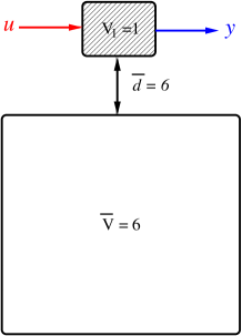
Figure 5: Simplified equivalent structure of the example

7.2 Example 2

Consider a network with one mobile zone and four immobile zones of identical volumes $V_{i}=1$ ($i=1\cdots 5$), as depicted on Figure 6 with the following diffusive exchange rates

$$d_{12}=1\ ,\;d_{13}=2\ ,\;d_{34}=1\ ,\;d_{35}=3\ ,\;d_{45}=1\ .$$

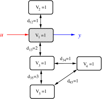
Figure 6: Example of a network with one mobile and four immobile zones

The structure of this network is neither MRMT nor MINC, and its corresponding matrix $A$ is

$$A=\left[\begin{array}[]{ccccc}-3&1&1&0&0\\ 1&-1&0&0&0\\ 1&0&-3&1&1\\ 0&0&1&-2&1\\ 0&0&1&1&-2\end{array}\right].$$

One can easily compute the controllability matrix

$${\cal C}_{A,B}=\left[\begin{array}[]{ccccc}1&-4&21&-129&906\\ 0&1&-5&26&-155\\ 0&2&-20&182&-1614\\ 0&0&2&-18&136\\ 0&0&6&-82&856\end{array}\right]$$

and check that it is full rank (computing for instance $det({\cal C}_{A,B})=-896$). Then, the constructions of Sections 5 and 6 give the following equivalent MRMT and MINC matrices:

$$A_{MRMT}=\left[\begin{array}[]{ccccc}-4&0.3256267&0.1692779&1&1.5050954\\ 8.1710298&-8.1710298&0&0&0\\ 3.3115831&0&-3.3115831&0&0\\ 1&0&0&-1&0\\ 0.5173871&0&0&0&-0.5173871\end{array}\right],$$

$$A_{MINC}=\left[\begin{array}[]{ccccc}-4&3&0&0&0\\ 1.6666667&-5&3.3333333&0&0\\ 0&3.6&-4.1333333&0.5333333&0\\ 0&0&2.4666667&-2.9207207&0.4540541\\ 0&0&0&0.9459459&-0.9459459\end{array}\right].$$

We have checked numerically that each matrix $A$, $A_{MRMT}$ and $A_{MINC}$ give the same co-prime transfer function

$$T(z)=\frac{14+47z+45z^{2}+13z^{3}+z^{4}}{14+117z+187z^{2}+92z^{3}+17z^{4}+z^{5}}.$$

Differently to the original network, the magnitude of the values of volumes and diffusive exchange rates are significantly different among compartments, opening the door of possible model reduction dropping some compartments.

1. For the equivalent MRMT structure, one obtains

   $$V_{1}=1\ ,\;V_{2}=0.0398514\ ,\;V_{3}=0.0511169\ ,\;V_{4}=1\ ,\;V_{5}=2.9090317$$

   with

   $$d_{12}=0.3256267\ ,\;d_{13}=0.1692779\ ,\;d_{14}=1,\;d_{15}=1.5050954$$

   and notices that zones $2$ and $3$ are of relatively small volumes (compared to the total volume of the system which is equal to $5$) and connected to the mobile zone with relatively small diffusive parameters. Then, one may expect to have a good approximation with a reduced MRMT model dropping zones $2$ and $3$. Keeping the volumes $V_{1}$, $V_{4}$, $V_{5}$ with the parameters $d_{14}$, $d_{15}$, one obtains the the 3 compartments MRMT matrix

   $$\tilde{A}_{MRMT}=\left[\begin{array}[]{ccc}-3.5050954&1&1.5050954\\ 1&-1&0\\ 0&0.5173871&-0.5173871\end{array}\right]$$

   with the corresponding transfer function

   $$\tilde{T}_{MRMT}(z)=\frac{0.5173871+1.5173871z+z^{2}}{0.5173871+4.8359736z+5.0224825z^{2}+z^{3}}\ .$$

2. For the equivalent MINC structure, one obtains

   $$V_{1}=1\ ,\;V_{2}=1.8\ ,\;V_{3}=1.6666667\ ,\;V_{4}=0.3603604\ ,\;V_{5}=0.1729730$$

   with

   $$d_{12}=3\ ,\;d_{23}=6\ ,\;d_{34}=0.8888889,\;d_{45}=0.1636231\ .$$

   Here, one notices that the two last volumes are relatively small and connected with relatively small diffusion terms. Keeping the volumes $V_{1}$, $V_{2}$, $V_{3}$ with the parameters $d_{12}$, $d_{23}$, one obtains the the 3 compartments MINC matrix

   $$\tilde{A}_{MINC}=\left[\begin{array}[]{ccc}-4&3&0\\ 1.6666667&-5&3.3333333\\ 0&3.6&-3.6\end{array}\right]$$

   with the corresponding transfer function

   $$\tilde{T}_{MINC}(z)=\frac{6+8.6z+z^{2}}{6+35.4z+12.6z^{2}+z^{3}}\ .$$

The Nyquist plots of the transfer functions $T$, $\tilde{T}_{MRMT}$ and $\tilde{T}_{MINC}$ are reported on Figure 7, showing the quality of the approximation with only three compartments derived from the MRMT or MINC representations. There exist many reduction methods in the literature, but a reduction through MRMT or MINC has the advantage to obtain easily reduced models with a physical meaning.

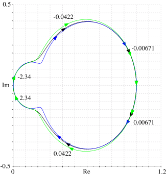
Figure 7: Nyquist diagrams (black: original system, blue: reduced MRMT, green: reduced MINC)

Remark 7.1.

For a positive linear system $(A,B)$, let ${\cal A}_{0}^{+}(A,B)$ be the attainability set from the $0$-state with non-negative controls. The system being positive, one has ${\cal A}_{0}^{+}(A,B)\subset\mathbb{R}_{+}^{n}$ and for any state $X\in{\cal A}_{0}^{+}(A,B)$, the state $Z=R^{-1}X$ for the equivalent MRMT or MINC structure is also non-negative, but for a state $X\in\mathbb{R}_{+}^{n}\setminus{\cal A}_{0}^{+}(A,B)$, the equivalent state $Z=R^{-1}X$ is not necessarily non-negative (as the coefficients of the matrix $R^{-1}$ are not necessarily non-negative). Consequently, one can have an equivalent input-output representation in MRMT form but with negative concentrations for such states of the system. Physically, this means that the compartments network has not been filled from a substrate-free state with a control $u(\cdot)$.This observation might be relevant from a geophysical view point.

8 Conclusion

We have shown that any general network structure is equivalent to a “star” structure (MRMT) or a “series” structure (MINC), that are commonly considered in geosciences to represent soil porosity in mass transfers. In this way, we reconcile these two different approaches, showing that they are indeed equivalent. Practically, this means that when the structure is unknown, or partially known, one can use equivalently the most convenient structure to identify the parameters or use some a priory knowledge.

In this work we have also shown the crucial role played the controllability property of a given mass transfer structure. Although there is no particular control issue in the input-output representations of mass transfers, controllability is a necessary condition to obtain equivalence with the multi-rate mass transfer (MRMT) structures of depth one, introduced by Haggerty and Gorelick in 1995 [18], or the multiple interacting continua structure (MINC). This condition is related to the minimal representation of linear systems, that is not necessarily fulfilled for such structures even for non-singular irreducible network matrices with distinct eigenvalues.

Although the objective of the present work is to show the exact equivalence of systems, we have shown on examples that MRMT and MINC representations could allow a simple and efficient way to obtain reduced models with a good approximation. Further investigations about such reduction techniques will be the matter of a coming work.

From a geosciences view point, this analysis shows the existence of both identifiable and non-identifiable porosity structures from input-output data. Input-output signals are typical of conservative tracer tests where non-reactive tracers are injected in an upstream well and analyzed in a downstream well [13]. Identifiable structures could thus be calibrated on tracer tests [1]. The porosity structure identified is however not unique as demonstrated on the example in Section 7, meaning that a porosity structure cannot be fully characterized by a tracer test. This is an advantage rather than a drawback for this class of models as the porosity structure should support both conservative and reactive transport [10, 9]. Reactive transport does not only depend on the input/output concentrations but also on the concentrations within the diffusion porosities, i.e. from the full state of the system. In a broader perspective, some further characteristics of the porosity structure might be revealed by reactive tracers used in combination with conservative tracers.

Acknowledgments.

This work was developed in the framework of the DYMECOS 2 INRIA Associated team and of project BIONATURE of CIRIC INRIA CHILE, and it was partially supported by CONICYT grants REDES 130067 and 150011. The second and fourth authors were also supported by CONICYT-Chile under ACT project 10336, FONDECYT 1160204 and 1160567, BASAL project (Centro de Modelamiento Matemático, Universidad de Chile), CONICYT national doctoral grant and CONICYT PAI/ Concurso Nacional Tesis de Doctorado en la Empresa, convocatoria 2014, 781413008.

The authors are grateful to T. Babey, D. Dochain J. Harmand, C. Casenave, J.L. Gouzé and B. Cloez for fruitful discussions and insightful ideas.

This research has been also conducted in the scope of the French ANR project Soil$\mu$3D.

References

• [1] D. Anderson, Compartmental Modeling and Tracer Kinetics, Lecture Notes in Biomathematics, Vol. 50, Springer, 1983.
• [2] T. Babey, J.-R. de Dreuzy and C. Casenave, Multi-Rate Mass Transfer (MRMT) models for general diffusive porosity structures, Advances in Water Resources, Vol. 76, pp. 146–156, 2015.
• [3] T. Babey, J.-R. de Dreuzy and T. R. Ginn, From conservative to reactive transport under diffusion-controlled conditions, Water Resources Research, Vol. 52(5), pp. 3685–3700, 2016.
• [4] L. Benvenuti, Minimal Positive Realizations of Transfer Functions With Real Poles, IEEE Trans. Autom. Control, vol. 58(4), pp. 1013–1017, 2013.
• [5] L. Benvenuti and L. Farina, A tutorial on the positive realization problem, IEEE Trans. Autom. Control, vol. 49(5), pp. 651-664, 2004.
• [6] A. Berman and R.J. Plemmons, Nonnegative Matrices in the Mathematical Sciences. SIAM Classics in Applied Mathematics, 1994.
• [7] J. Carrera, X. Sanchez-Vila, I. Benet, A. Medina, G. Galarza and J. Guimera, On matrix diffusion: formulations, solution methods and qualitative effects, Hydrogeology Journal, Vol. 6(1), pp. 178–190, 1998.
• [8] K. Coats and B. Smith Dead-end pore volume and dispersion in porous media. Society of Petroleum Engineers Journal, Vol. 4(1), pp. 73–84, 1964.
• [9] L. Donado, X. Sanchez-Vila, M. Dentz, J. Carrera and D. Bolster, Multi-component reactive transport in multicontinuum media, Water Resources Research, Vol. 45(11), pp. 1–11, 2009.
• [10] J.-R. de Dreuzy, A. Rapaport, T. Babey, J. Harmand, Influence of porosity structures on mixing-induced reactivity at chemical equilibrium in mobile/immobile Multi-Rate Mass Transfer (MRMT) and Multiple INteracting Continua (MINC) models, Water Resources Research, Vol. 49(12), pp. 8511–8530, 2013.
• [11] G. de Marsily, Quantitative Hydrogeology: Groundwater Hydrology for Engineers, Academic Press, Orlando, 1986.
• [12] L. Farina and S. Rinaldi, Positive Linear Systems, Theory and Applications, Prentice Hall, 2000.
• [13] C. Fetter, Contaminant Hydrogeology, (2nd edition). Waveland Pr Inc., 2008.
• [14] L. Gelhar, Stochastic Subsurface Hydrology Prentice Hall, Engelwood Cliffs, New Jersey, 1993.
• [15] L. Gelhar, C. Welty and R. Rhefeldt, A Critical Review of Data on Field-Scale Dispersion in Aquifers. Water Resources Research, Vol. 28(7), pp. 1955–1974, 1992.
• [16] G. Golub, B. Kågström and P. Van Dooren, Direct block tridiagonalization of single-input single-output systems. Systems & Control Letters, Vol. 18, pp. 109–120, 1992.
• [17] G. Golub and C. Van Loan, Matrix Computations. The Johns Hopkins University Press, 4th. ed, 2013.
• [18] R. Haggerty and S. Gorelick, Multiple-rate mass transfer for modeling diffusion and surface reactions in media with pore-scale heterogeneity, Water Resources Research, Vol. 31(10), pp. 2383–2400, 1995.
• [19] R. Horn and C. Johnson, Matrix Analysis, Cambridge University Press, 1985.
• [20] J. Jacquez and C. Simon Qualitative theory of compartmental systems, SIAM Review, Vol. 35(1), pp. 43–79 , 1993.
• [21] T. Kailath, Linear Systems, Prentice Hall, 1980.
• [22] K. Maher, The role of fluid residence time and topographic scales in determining chemical fluxes from landscapes, Earth and Planetary Science Letters, 312(1–2), pp. 48–58, 2011.
• [23] S. Marsili-Libelli, Environmental Systems Analysis with MATLAB. CRC Press, 2016.
• [24] S. McKenna, L. Meigs and R. Haggerty, Tracer tests in a fractured dolomite 3. Double-porosity, multiple-rate mass transfer processes in convergent flow tracer tests Water Resources Research, Vol. 37(5), pp. 1143–1154, 2001.
• [25] B. Nagy and M. Matolcsi, Minimal positive realizations of transfer functions with nonnegative multiple poles, IEEE Trans. Autom. Control, Vol. 50(9), pp. 1447-1450, 2005.
• [26] K. Pruess and T. Narasimhan, A practical method for modeling fluid and heat-flow in fractured porous-media, Society of Petroleum Engineers Journal, Vol. 25(1), pp. 14–26, 1985.
• [27] C. Steefel, D. De Paolo and P. Lichtner, Reactive transport modeling: An essential tool and a new research approach for the Earth sciences, Earth and Planetary Science Letters, Vol. 240(3-4), pp. 539–558., 2005.
• [28] C. Steefel and K. Maher, Fluid-Rock Interaction: A Reactive Transport Approach, in Thermodynamics and Kinetics of Water-Rock Interaction, edited by E. H. Oelkers and J. Schott, pp. 485-532, Mineralogical Soc. Amer., Chantilly, pp. 485–532, 2009.
• [29] M. Vangenuchten and J. Wierenga, Mass-transfer studies in sorbing porous-media .1. Analytical solutions, Soil Science Society of America Journal, Vol. 40(4), pp. 473–480, 1976.
• [30] G. Walter and M. Contreras, Compartmental Modeling with Networks, Birkäuser, 1999.
• [31] J. Warren, P. Root and M. Aime, The Behavior of Naturally Fractured Reservoirs, Society of Petroleum Engineers Journal, Vol. 3(3), pp. 245–255, 1963.
• [32] M. Willmann, J. Carrera, X. Sanchez-Vila, O. Silva and M. Dentz, Coupling of mass transfer and reactive transport for nonlinear reactions in heterogeneous media, Water Resources Research, Vol. 46(7), pp. 1–15, 2010.
• [33] B. Zinn, L. Meigs, C. Harvey, R. Haggerty, W. Peplinski and C. von Schwerin, Experimental visualization of solute transport and mass transfer processes in two-dimensional conductivity fields with connected regions of high conductivity, Environmental Science & Technology, Vol. 38(14), pp. 3916–3926, 2004.