Approximation of the weighted maximin dispersion problem over $\ell_{p}-$ball: SDP relaxation is misleading

Abstract

Consider the problem of finding a point in a unit $n$-dimensional $\ell_{p}$-ball ($p\geq 2$) such that the minimum of the weighted Euclidean distance from given $m$ points is maximized. We show in this paper that the recent SDP-relaxation-based approximation algorithm [SIAM J. Optim. 23(4), 2264-2294, 2013] will not only provide the first theoretical approximation bound of $\frac{1-O\left(\sqrt{\ln(m)/n}\right)}{2}$, but also perform much better in practice, if the SDP relaxation is removed and the optimal solution of the SDP relaxation is replaced by a simple scalar matrix.

1 Introduction

As is well-known, following the pioneer work on providing a $0.878$-approximate solution for max-cut problem GW95 , the semidefinite programming (SDP) relaxation technique has been playing a great role in approximately solving combinatorial optimization problems and nonconvex quadratic programs; see for example, GJ ; Luo ; Nem ; Ne ; Ye .

This paper is to present a surprise case where the SDP relaxation misleads the approximation in both theory and computation.

Consider the $\ell_{p}$-ball ($p\geq 2$) constrained weighted maximin dispersion problem:

$${\rm(P)}~{}~{}\max_{\|x\|_{p}\leq 1}\left\{f(x):=\min_{i=1,\ldots,m}\omega_{i}\|x-x^{i}\|_{2}^{2}\right\},$$

where $x^{1},\ldots,x^{m}\in\mathbb{R}^{n}$ are given $m$ points, $\omega_{i}>0$ for $i=1,\ldots,m$, and $\|x\|_{p}:=\left(\sum_{i=1}^{n}|x_{i}|^{p}\right)^{\frac{1}{p}}$ is the $\ell_{p}$-norm of $x$. Applications of (P) can be found in facility location, spatial management, and pattern recognition; see DW ; JMY ; Sc ; W and references therein.

Based on the SDP relaxation technique, Haines et al. HA13 proposed the first approximation algorithm for solving (P). However, their approximation bound is not so clean that it depends on the optimal solution of the SDP relaxation. Fortunately, when $p=+\infty$, the approximation bound reduces to

$$\frac{1-O\left(\sqrt{\frac{\ln(m)}{n}}\right)}{2}.$$ (1)

Very recently, the above approximation bound (1) is established for the special case $p=2$ based on a different algorithm WX16 . But further extension to (P) with $p>2$ remains open WX16 .

In this paper, we show that, by removing the SDP relaxation from Haines et al.’s approximation algorithm HA13 and simply replacing the optimal solution of the SDP relaxation with a scalar matrix, the approximation bound (1) becomes to be satisfied for (P). It is the SDP relaxation that makes the whole approximation algorithm not only loses the theoretical bound (1) but also performs poorly in practice.

The remainder of this paper is organized as follows. In Section 2, we present the existing approximation algorithm based on SDP relaxation. In Section 3, we propose a new simple approximation algorithm without any convex relaxation and establish the approximation bound. Numerical comparison is reported in Section 4. We make conclusions in Section 5.

Throughout this paper, we denote by $\mathbb{R}^{n}$ and $S^{n}$ the $n$-dimensional real vector space and the space of $n\times n$ real symmetric matrices, respectively. Let $I_{n}$ be the identity matrix of order $n$. $A\succ(\succeq)0$ denotes that $A$ is positive (semi)definite. The inner product of two matrices $A$ and $B$ is denoted by $A\bullet B={\rm Tr}(AB^{T})=\sum_{i=1}^{n}\sum_{j=1}^{n}a_{ij}b_{ij}$. ${\rm Pr(\cdot)}$ stands for the probability.

2 Approximation algorithm based on SDP relaxation

In this section, we present Haines et al.’s randomized approximation algorithm HA13 based on SDP relaxation.

It is not difficult to verify that lifting $xx^{T}$ to $X\in S^{n}$ yields the SDP relaxation for (P):

$${\rm(SDP)}~{}~{} \max_{X,x} ~{}\min\left\{\omega_{i}\left(\begin{array}[]{cc}I_{n}&-x^{i}\\ -(x^{i})^{T}&\|x^{i}\|_{2}^{2}\end{array}\right)\bullet\left(\begin{array}[]{cc}X&x\\ x^{T}&1\end{array}\right)\right\}$$

$${\rm s.~{}t.} X_{11}^{\frac{p}{2}}+X_{22}^{\frac{p}{2}}+\ldots+X_{nn}^{\frac{p}{2}}\leq 1,$$

$$\left(\begin{array}[]{cc}X&x\\ x^{T}&1\end{array}\right)\succeq 0.$$

Since it is assumed that $p\geq 2$, the above (SDP) is a convx program and hence can be solved efficiently NN .

Now, we present Haines et al.’s SDP-based approximation algorithm HA13 for solving (P).

Algorithm 1: SDP-based approximation algorithm HA13 . 1.  Input $\rho\in(0,1)$ and $x^{i}$ for $i=1,\ldots,m$. Let $\alpha=\sqrt{2\ln(m/\rho)}$. 2.  Solve ${\rm(SDP)}$ and return the optimal solution $X^{*}\in S^{n}$. Set       $b^{i}=(\sqrt{X^{*}_{11}}x^{i}_{1},\ldots,\sqrt{X^{*}_{nn}}x^{i}_{n})^{T}$ for $i\in\{1,\ldots,m\}\setminus\{k\mid\|x^{k}\|=0\}$. 3.  Repeatedly generate $\xi=(\xi_{1},\ldots,\xi_{n})^{T}$ with independent $\xi_{i}$ taking      the value $\pm 1$ with equal probability until $(b^{i})^{T}\xi<\alpha\|b^{i}\|$ for       $i\in\{1,\ldots,m\}\setminus\{k\mid\|x^{k}\|=0\}$. 4.  Output $\widetilde{x}=\left(\sqrt{{X^{*}_{11}}}\xi_{1},\sqrt{{X^{*}_{22}}}\xi_{2},\ldots,\sqrt{{X^{*}_{nn}}}\xi_{n}\right)^{T}$.

Remark 1

The original version of the above algorithm HA13 did not consider the possible case $\|x^{k}\|=0$ for some $k$. It has been fixed in WX16 .

Remark 2

The existence of $\xi$ in Step 3 of Algorithm $1$ is guaranteed by the inequality HA13 :

$${\rm Pr}\left((b^{i})^{T}\xi<\alpha\|b^{i}\|,~{}i\in I\right)\geq 1-\rho>0,$$

which is a trivial corollary of the following well-known result.

Theorem 1

(Ben2002, , Lemma A.3) Let $\xi\in\{-1,1\}^{n}$ be a random vector, componentwise independent, with

$${\rm Pr}(\xi_{j}=1)={\rm Pr}(\xi_{j}=-1)=\frac{1}{2},~{}\forall j=1,\ldots,n.$$

Let $b\in\mathbb{R}^{n}$ and $\|b\|>0$. Then, for any $\alpha>0$,

$${\rm Pr}(b^{T}\xi\geq\alpha\|b\|)\leq e^{-\alpha^{2}/2}.$$

For the approximation bound of Algorithm 1, the following main result holds.

Theorem 2

(HA13, , Theorem 3) For the solution $\widetilde{x}$ returned by the Algorithm 1, we have

$$v({\rm P})\geq f(\widetilde{x})\geq\frac{1-\sqrt{2\gamma_{1}^{*}\ln(m/\rho)}}{2}v({\rm P}).$$

where $\gamma_{1}^{*}=\frac{\max_{j=1,\ldots,n}X^{*}_{jj}}{\sum_{j=1}^{n}X^{*}_{jj}}$. Moreover, when $p=+\infty$, $\gamma_{1}^{*}=\frac{1}{n}$.

Finally, we remark that the equality $\gamma_{1}^{*}=\frac{1}{n}$ is no longer true when $p<+\infty$. The following counterexample is taking from WX16 .

Example 1

(WX16, , Example 4.1) Let $n=2,~{}m=3$, $p=2$, $x^{1}=\left(\begin{array}[]{c}1\\ 2\end{array}\right)$, $x^{2}=\left(\begin{array}[]{c}2\\ 3\end{array}\right)$, $x^{3}=\left(\begin{array}[]{c}1\\ 5\end{array}\right)$, and $\omega_{1}=\omega_{2}=\omega_{3}=1$. Solving (SDP), we obtain

$$\gamma_{1}^{*}=0.8>0.5=\frac{1}{n}.$$

Moreover, the above value of $\gamma_{1}^{*}$ is unique. For the detail of the verification, we refer the reader to WX16 .

3 Approximation algorithm without convex relaxation

In this section, we propose a simple randomized approximation algorithm for solving (P). We remove the SDP relaxation from Algorithm 1 and then replace the optimal solution $X^{*}$ with the scalar matrix $n^{-\frac{2}{p}}I_{n}$. It turns out that our new algorithm just uniformly and randomly pick a solution from $\{n^{-\frac{1}{p}}(t_{1},t_{2},\ldots,t_{n})^{T}\mid~{}t_{i}=-1~{}{\rm or}~{}1,~{}i=1,\ldots,n\}$, which is a set of $2^{n}$ points on the surface of the unit $\ell_{p}$-ball. The detailed algorithm is as follows.

Algorithm 2: Approximation algorithm without convex relaxation. 1.  Input $\rho\in(0,1)$ and $x^{i}$ for $i=1,\ldots,m$. Let $\alpha=\sqrt{2\ln(m/\rho)}$. 2.  Repeatedly generate $\xi\in\mathbb{R}^{n}$ with independent $\xi_{i}$ taking $\pm 1$ with equal      probability until $(x^{i})^{T}\xi<\alpha\|x^{i}\|$ for $i\in\{1,\ldots,m\}\setminus\{k\mid\|x^{k}\|=0\}$. 3.  Output $\widetilde{x}=n^{-\frac{1}{p}}\xi.$

Surprisingly, for any $p\geq 2$, we can show that our new Algorithm 2 always provides the approximation bound (1) for (P).

Theorem 3

Let $p\geq 2$. For the solution $\widetilde{x}$ returned by Algorithm 2, we have

$$v({\rm P})\geq f(\widetilde{x})>\frac{1-\sqrt{\frac{2}{n}\ln(m/\rho)}}{2}\cdot v({\rm P}).$$

Proof

According to the settings in Algorithm 2, for $i\in\{1,\ldots,m\}$ such that $\|x^{i}\|>0$, we have

$$\|\widetilde{x}-x^{i}\|_{2}^{2} = \|\widetilde{x}\|_{2}^{2}-2(x^{i})^{T}\widetilde{x}+\|x^{i}\|_{2}^{2}$$ (4)

$$\geq \|\tilde{x}\|_{2}^{2}-2\alpha\|x^{i}\|_{2}\cdot n^{-\frac{1}{p}}+\|x^{i}\|_{2}^{2}$$

$$= n^{1-\frac{2}{p}}-2\alpha\|x^{i}\|_{2}\cdot n^{-\frac{1}{p}}+\|x^{i}\|_{2}^{2}$$

$$\geq (n^{1-\frac{2}{p}}+\|x^{i}\|_{2}^{2})(1-\alpha\cdot n^{-\frac{1}{2}}),$$

where the inequality (4) holds since according to the Cauchy-Schwarz inequality, it holds that

$$2\|x^{i}\|_{2}\cdot n^{\frac{1}{2}-\frac{1}{p}}\leq n^{1-\frac{2}{p}}+\|x^{i}\|_{2}^{2}.$$ (5)

If there is an index $k$ such that $\|x^{k}\|_{2}=0$, we have

$$\|\tilde{x}-x^{k}\|_{2}^{2}=n^{1-\frac{2}{p}}>(n^{1-\frac{2}{p}}+\|x^{k}\|_{2}^{2})(1-\alpha\cdot n^{-\frac{1}{2}}).$$ (6)

Next, let $x^{*}$ be an optimal solution of (P). Then, for $i=1,\ldots,m$ and $\|x^{i}\|>0$, it holds that

$$v({\rm P}) \leq {\omega_{i}}(\|x^{*}\|_{2}^{2}-2(x^{i})^{T}x^{*}+\|x^{i}\|_{2}^{2})$$ (7)

$$\leq {\omega_{i}}(n^{1-\frac{2}{p}}-2(x^{i})^{T}x^{*}+\|x^{i}\|_{2}^{2})$$

$$\leq {\omega_{i}}(n^{1-\frac{2}{p}}+2\|x^{i}\|_{2}\cdot\|x^{*}\|_{2}+\|x^{i}\|_{2}^{2})$$

$$\leq {\omega_{i}}(n^{1-\frac{2}{p}}+2\|x^{i}\|_{2}n^{\frac{1}{2}-\frac{1}{p}}+\|x^{i}\|_{2}^{2})$$

$$\leq 2{\omega_{i}}(n^{1-\frac{2}{p}}+\|x^{i}\|_{2}^{2}),$$ (9)

where the inequality (7) holds since it follows from the Hölder inequality that

$$\|x^{*}\|_{2}^{2}\leq\left(\sum_{i=1}^{n}(x_{i}^{*2})^{\frac{p}{2}}\right)^{\frac{2}{p}}\left(\sum_{i=1}^{n}1^{\frac{p}{p-2}}\right)^{1-\frac{2}{p}}=\left(\sum_{i=1}^{n}|x^{*}_{i}|^{p}\right)^{\frac{2}{p}}n^{1-\frac{2}{p}}\leq n^{1-\frac{2}{p}},$$

the inequality (3) holds due to the Cauchy-Schwarz inequality and the inequality (9) follows from (5). For the case that there is an index $k$ such that $\|x^{k}\|=0$, we also have

$$v({\rm P})\leq\omega_{k}(n^{1-\frac{2}{p}}-2(x^{k})^{T}x^{*}+\|x^{k}\|_{2}^{2})=\omega_{k}\cdot n^{1-\frac{2}{p}}<2\omega_{k}(n^{1-\frac{2}{p}}+\|x^{k}\|_{2}^{2}).$$ (10)

Thus, it follows from (4), (6), (9) and (10) that

$$\min_{i=1,\ldots,m}\omega_{i}\|\tilde{x}-x^{i}\|_{2}^{2}>\frac{1-\alpha\cdot n^{-\frac{1}{2}}}{2}\cdot v({\rm P}).$$ (11)

Substituting $\alpha=\sqrt{2\ln(m/\rho)}$ in (11) completes the proof.

Remark 3

Theorem 3 implies that Algorithm 2 provides a $1/2$ asymptotic approximation bound for (${\rm P}$) as $\frac{n}{\ln(m)}$ increases to infinity.

4 Numerical Experiments

In this section, we numerically compare our new simple approximation algorithm (Algorithm 2) with the SDP-based algorithm proposed in HA13 (i.e., Algorithm 1 in this paper) for solving (P). In Algorithm 1, we use SDPT3 within CVX GrB to solve $({\rm SDP})$. All the numerical tests are constructed in MATLAB R2013b and carried out on a laptop computer with $2.3$ GHz processor and $4$ GB RAM.

First, we fix $p=3$, $n=20$, and $\omega_{1}=\omega_{2}=\ldots=\omega_{m}=1$. Then, we randomly generate the test instances where $m$ varies in $\{10,12,\ldots,30\}$. Since all of the input points $x^{i}~{}(i=1,\ldots,m)$ with $m=10,12,\ldots,30$ form an orderly $n\times 220$ matrix. We generate this random matrix using the following Matlab scripts:

              rand(’state’,0); X = 2*rand(n,220)-1;

For each instance, we independently run each of the two algorithms $20$ times with the same setting $\rho=0.9999$ and then plot the objective values of the returned approximation solutions in Figure 1.

Second, we fix $n=20,~{}m=30$, $\omega_{1}=\omega_{2}=\ldots=\omega_{m}=1$, and let $p=2,3,5,10,20,50,100,200,500,800,1000$. The total $30$ input points $x^{i}~{}(i=1,\ldots,m)$ are generated using the following Matlab scripts:

              rand(’state’,0); X = 2*rand(n,30)-1;

Both Algorithm 1 and Algorithm 2 are then independently implemented $20$ times for each $p$ with the same setting $\rho=0.9999$. We plot the objective values of the returned approximation solutions in Figure 2.

According to Figures 1 and 2, the qualities of the approximation solutions returned by Algorithm 2 are in general much higher than those generated by Algorithm 1. The practical performance demonstrates that at least for finding approximation solutions of (P), the SDP relaxation is misleading.

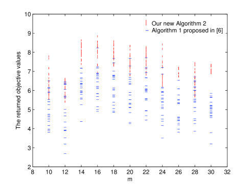
Figure 1: Approximation solutions returned by the SDP-based Algorithm 1 and our new simple Algorithm 2 with different $m$.

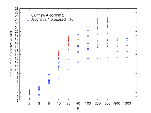
Figure 2: Approximation solutions returned by the SDP-based Algorithm 1 and our new simple Algorithm 2 with different $p$.

5 Conclusions

In this paper, we propose a new simple approximation algorithm for the $\ell_{p}$-ball constrained weighted maximin dispersion problem (P). It is inherited from the existing SDP-based algorithm by removing the SDP relaxation and then trivially replacing the optimal solution of the SDP relaxation with a particular scalar matrix. Surprisingly, the simplified algorithm can provide the first unified approximation bound of $\frac{1-O\left(\sqrt{\ln(m)/n}\right)}{2}$ for any $2\leq p\leq+\infty$, which remains open up to now except for the special cases $p=2$ and $p=+\infty$. Numerical results also imply that the SDP relaxation technique is misleading in approximately solving (P). Finally, we raise a question whether the unified approximation bound can be extended to (P) with $1\leq p<2$.

References

- (1) Ben-Tal, A., Nemirovski A., Roos, C.: Robust solutions of uncertain quadratic and conic-quadratic problems. SIAM J. Optim., 13, 535–560 (2002)
- (2) Dasarathy, B., White, L.J.: A maximin location problem. Oper. Res. 28, 1385–1401 (1980)
- (3) Gärtner, B., Matousek, J.: Approximation Algorithms and Semidefinite Programming. Diss. Springer Berlin Heidelberg, 2012.
- (4) Goemans, M.X., Williamson, D.P.: Improved approximation algorithms for maximum cut and satisfiability problems using semidefinite programming. J. ACM, 42, 1115–1145 (1995)
- (5) Grant, M., Boyd, S.: CVX: Matlab software for disciplined convex programming, version 2.1, http://cvxr.com/cvx, June 2015.
- (6) Haines, S., Loeppky, J., Tseng, P., Wang, X.: Convex relaxations of the weighted maxmin dispersion problem. SIAM J. Optim. 23(4), 2264–2294 (2013)
- (7) Johnson, M.E., Moore, L.M., Ylvisaker, D.: Minimax and maximin distance designs. J. Satist. Plan. Inference. 26, 131–148 (1990)
- (8) Luo, Z.Q., Ma, W.K., So, A.M.C., Ye, Y., Zhang, S.Z.: Semidefinite relaxation of quadratic optimization problems. IEEE Signal Process. Mag., 27(3), 20–34 (2010)
- (9) Nemirovski, A., Roos, C., Terlaky, T.: On maximization of quadratic form over intersection of ellipsoids with common center, Math. Program. 86, 463–473 (1999)
- (10) Nesterov, Y.: Semidefinite relaxation and nonconvex quadratic optimization, Optim. Methods Softw., 9, 141–160 (1998)
- (11) Nesterov, Y., Nemirovsky, A.: Interior-Point Polynomial Methods in Convex Programming, SIAM, Philadelphia, PA, 1994.
- (12) Schaback, R.: Multivariate Interpolation and Approximation by Translates of a Basis Function, in Approximation Theory VIII, C. K. Chui and L. L. Schumaker eds., World Scientific, Singapore, 491–514 (1995)
- (13) White, D.J.: A heuristic approach to a weighted maxmin dispersion problem. IMA J. Math. Appl. Business and Industry. 7, 219–231 (1996)
- (14) Wang, S., Xia, Y.: On the Ball-Constrained Weighted Maximin Dispersion Problem. SIAM J. Optim., in press (2016)
- (15) Ye, Y.: Approximating quadratic programming with bound and quadratic constraints, Math. Program., 84, 219–226 (1999)