Concordance group of virtual knots

Abstract.

We study concordance of virtual knots. Our main result is that a classical knot $K$ is virtually slice if and only if it is classically slice. From this we deduce that the concordance group of classical knots embeds into the concordance group of long virtual knots.

1. Introduction

Virtual knot theory, discovered by Kauffman [Ka99], is a nontrivial extension of classical knot theory. Indeed, Goussarov, Polyak, and Viro proved that any two classical knots are equivalent as virtual knots if and only if they are equivalent as classical knots [GPV00, Theorem 1.B]. Their result served to motivate many subsequent developments, because it predicted that many classical knot and link invariants can be extended to virtual knots and links.

This result from [GPV00] was originally deduced from the classical Waldhausen’s theorem [Wa68, Corollary 6.5], but it can also be derived from Kuperberg’s theorem [Ku03]. In the latter formulation, one represents virtual knots geometrically as knots in thickened surfaces up to stable equivalence, and Kuperberg’s theorem tells us that the minimal genus representative is unique up to diffeomorphism.

Concordance of virtual knots has recently become an area of active interest, and many basic questions are still open. One important question, which was raised both by Turaev [Tu08, Section 2.2] and by Kauffman [Ka15, p. 336], is the following: If two classical knots are concordant as virtual ones, are they concordant in the usual sense? Our main result gives an affirmative answer to this question.

Theorem.

If two classical knots are concordant as virtual knots, then they are also concordant as classical knots.

This result can be viewed as the analogue in concordance of the earlier result of Goussarov, Polyak, and Viro [GPV00], and consequently we hope that it will stimulate further research on the problem of extending concordance invariants from the classical to the virtual setting. In fact, there are already exciting new developments along these lines, for instance the extension of the Rasmussen $s$-invariant to virtual knots given by Dye, Kaestner, and Kauffman [DKK14].

We give a brief overview of the rest of the paper. In Section 2, we introduce virtual knots as knots in thickened surfaces up to stable equivalence. We recall Turaev’s definition of virtual knot concordance in Subsection 2.2, and we state and prove our main result in Subsection 2.3. In Section 3, we introduce long virtual knots and construct the virtual knot concordance group $\mathscr{V}\!\mathscr{C}.$ We show that a long virtual knot $K$ is virtually slice if and only if its closure $\overline{K}$ is, and we use it to deduce injectivity of the natural homomorphism $\psi\colon\mathscr{C}\to\mathscr{V}\!\mathscr{C}$ from the classical concordance group to the virtual concordance group.

Conventions.

All manifolds are assumed smooth and all knots are assumed oriented. Throughout the paper, we work with smooth concordance.

2. Virtual knots and concordance

In this section, we introduce stable equivalence of knots in thickened surfaces and use them to define virtual knots. This gives rise to a natural notion of concordance for virtual knots, which allows for a bordism between the two surfaces whose thickenings contain representatives of the two virtual knots, and requires also an embedded annulus cobounding the two knots.

2.1. Diagrams and stable equivalence

It will be convenient for us to regard virtual knots geometrically as knots in thickened surfaces, and we take a moment to explain this point of view.

Definition 2.1.

A thickened surface $\Sigma\times I$ is a product of a closed, connected, oriented surface $\Sigma$ with the interval $I=[-1,1]$. A knot $K$ in a thickened surface $\Sigma\times I$ is a $1$-dimensional submanifold $K$ in the interior of $\Sigma\times I$ which is diffeomorphic to a circle.

Just as classical knots in $S^{3}$ are considered up to ambient isotopy, we consider knots in thickened surfaces up to stable equivalence [CKS02]. We take a moment to recall this carefully.

Definition 2.2.

Stable equivalence on knots in thickened surfaces is generated by the following operations, which transform a given knot $K$ in a thickened surface $\Sigma\times I$ into a new knot $K^{\prime}$ in a possibly different thickened surface $\Sigma^{\prime}\times I$.

1. Let $f\colon\Sigma\times I\to\Sigma^{\prime}\times I$ be an orientation-preserving diffeomorphism sending the orientation class of $\Sigma$ to that of $\Sigma^{\prime}$. (Notice that this implies that $f(\Sigma\times\{1\})=\Sigma^{\prime}\times\{1\}$ and $f(\Sigma\times\{-1\})=\Sigma^{\prime}\times\{-1\}$.) The knot $K^{\prime}=f(K)$ in $\Sigma^{\prime}\times I$ is said to be obtained from $K$ in $\Sigma\times I$ by a diffeomorphism.

2. Let $h\colon S^{0}\times D^{2}\to\Sigma$ be the attaching region for a $1$-handle that is disjoint from the image of $K$ under projection $\Sigma\times I\to\Sigma$, then $0$-surgery on $\Sigma$ along $h$ is the surface

   $$\Sigma^{\prime}:=\Sigma\smallsetminus h(S^{0}\times D^{2})\cup_{S^{0}\times S^{1}}D^{1}\times S^{1}.$$

   The knot $K^{\prime}$ is the image of the knot $K$ in $\Sigma^{\prime}\times I$, and we say that it is the knot obtained from $K$ by stabilisation.

3. Destabilisation is the inverse operation, and it involves cutting $\Sigma\times I$ along a vertical annulus $A$ and attaching two copies of $D^{2}\times I$ along the two annuli. If the resulting thickened surface is disconnected, then we keep only the component containing $K$.

Note that in (3), an annulus $A$ in $\Sigma\times I$ is called vertical if there is an embedded circle $\gamma\subset\Sigma$ such that $A=\gamma\times I\subset\Sigma\times I$. An equivalence class under the equivalence relation generated by (1), (2), and (3) above is called a virtual knot.

Virtual links admit a similar description as links in $\Sigma\times I$, though $\Sigma$ need not be connected. We abuse notation slightly and use $K$ for the virtual knot, so $K$ refers to an equivalence class of knots in thickened surfaces.

Given a virtual knot $K$, then any knot in its equivalence class will be called a representative for $K$. A representative is therefore a knot in a thickened surface $\Sigma\times I$.

Definition 2.3.

The virtual genus of a virtual knot $K$ is the minimum

$$vg(K):=\min\{g(\Sigma)\mid\text{$\Sigma\times I$ contains a representative for $K$}\},$$

where $g(\Sigma)$ denotes the genus of the surface $\Sigma$.

A classical knot $K\subset S^{3}$ can be isotoped to be disjoint from the two points $\{0,\infty\}$. Thus, we can view it as a knot in the thickened surface $S^{2}\times I$. The associated virtual knot is independent of the choice of isotopy, and we call such a knot classical. Therefore a virtual knot is classical if and only if its virtual genus is zero.

Kuperberg [Ku03, Theorem 1] proved a strong uniqueness result for minimal genus representatives. Namely, he showed that if $(K,\Sigma\times I)$ and $(K^{\prime},\Sigma^{\prime}\times I)$ are two minimal genus representatives for the same virtual knot, then $K^{\prime}=f(K)$ for some diffeomorphism $f\colon\Sigma\times I\to\Sigma^{\prime}\times I$ as in (1) of Definition 2.2 above.

For the sake of completeness, we relate the geometric definition of virtual knots to the usual diagrammatic definition.

A virtual knot diagram is a regular immersion of the circle $S^{1}$ in the plane ${\mathbb{R}}^{2}$ with double points that are either classical or virtual. Real crossings are drawn with one arc over the other whereas virtual crossings are drawn with circles around them.

Two virtual knot diagrams are equivalent if they are related by planar isotopies and generalised Reidemeister moves. These consist of the three usual Reidemeister moves together with three additional moves just like the usual Reidemeister moves but with only virtual crossings, and one more move called the mixed move which is depicted in Figure 1. A virtual knot is defined to be an equivalence class of virtual knot diagrams, and virtual links are defined similarly as equivalence classes of virtual link diagrams.

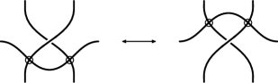
Figure 1. The mixed move.

Given a virtual knot diagram $D$ of a virtual knot $K$, there is a canonical surface $\Sigma$ called the Carter surface constructed from $D$ as follows [KK00]: attach two intersecting bands at every classical crossing and two non-intersecting bands at every virtual crossing as in Figure 2. Attaching non-intersecting and non-twisted bands along the remaining arcs of $D$, and filling in all boundary components with 2-disks, we obtain a closed oriented surface $\Sigma$ whose thickening $\Sigma\times I$ contains a representative of $K$. Conversely, let $K$ be a knot in a thickened surface $\Sigma\times I$ and $U\subset\Sigma$ a neighbourhood of the image of $K$ under projection $\Sigma\times I\to\Sigma$. If $f\colon U\to{\mathbb{R}}^{2}$ is an orientation preserving immersion, then the image of $K$ under $f$ is a virtual knot diagram $D$ whose classical crossings correspond to those of $K$ and whose virtual crossings, which are the rest of them, are the result of the immersion $f$. This virtual knot diagram $D$ depends on the choice of immersion $f$, but any two such diagrams are equivalent via detour moves [Ka15].

This establishes a one-to-one correspondence between virtual knot diagrams modulo the generalised Reidemeister moves and knots in thickened surfaces up to stable equivalence [CKS02].

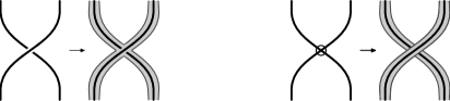
Figure 2. The bands for classical and virtual crossings.

2.2. Virtual concordance

In this section, we define concordance and sliceness for virtual knots in terms of their representative knots in thickened surfaces. We follow Turaev [Tu08, Section 2.1] in defining virtual knot concordance.

If $K$ is an oriented knot in a thickened surface $\Sigma\times I$, its reverse is the knot $K^{r}$ obtained by changing the orientation of $K$, and its mirror image is the knot $K^{m}$ obtained by changing the orientation of $\Sigma\times I$. These operations commute with one another, and we use $-K=K^{rm}$ to denote the knot obtained by taking the mirror image of the reverse knot.

Definition 2.4.

1. Two given knots $K_{0}\subset\Sigma_{0}\times I$ and $K_{1}\subset\Sigma_{1}\times I$ in thickened surfaces are virtually concordant if there exists a connected oriented $3$-manifold $W$ with $\partial W\cong-\Sigma_{0}\sqcup\Sigma_{1}$ and an annulus $A\subset W\times I$ cobounding $-K_{0}$ and $K_{1}$.

2. A knot $K\subset\Sigma\times I$ is called virtually slice if it is concordant to the unknot. Equivalently, the knot $K$ is virtually slice if there exists a connected $3$-manifold $W$ with $\partial W\cong\Sigma$ and a 2-disk $\Delta\subset W\times I$ cobounding $K$. We call $\Delta$ a slice disk for $K$.

Clearly, virtual concordance is an equivalence relation on knots in thickened surfaces. For instance, transitivity follows by stacking the two concordances in the usual way. The next result shows that two stably equivalent knots are virtually concordant to one another. Thus, it follows that virtual concordance defines an equivalence relation on virtual knots.

Lemma 2.5.

Suppose $K_{0}\subset\Sigma_{0}\times I$ and $K_{1}\subset\Sigma_{1}\times I$ represent the same virtual knot. Then $K_{0}$ and $K_{1}$ are virtually concordant.

Proof.

It is enough to find a 3-manifold $W$ and an annulus $A\subset W\times I$ realising a concordance between knots in surfaces transformed into each other by one of the operations generating stable equivalence, see Definition 2.2.

One can verify that this is possible in each case. ∎

Kauffman [Ka15] re-expressed concordance purely in terms of virtual knot diagrams. A concordance between two virtual knot diagrams $K_{0}$ and $K_{1}$ consists of a series of generalised Reidemeister moves together with a collection of saddle moves, births, and deaths that transform $K_{0}$ into $K_{1}$. As usual, one requires that the total number of births and deaths equals the number of saddle moves, see [Ka15, Section 3]. This condition is equivalent to the requirement that the knots cobound an annulus.

Example 2.6.

To illustrate this, we recall from [Ka15] the argument that the Kishino knot $K$ is virtually slice. To see this, perform a saddle move along the dotted line on the left of Figure 3. The result is a virtual link diagram on the right, which is easily seen to be equivalent to the unlink with two components. Filling them in with 2-disks gives a slice disk for $K$, showing that the Kishino knot is virtually slice.

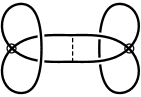
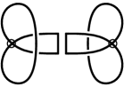
Figure 3. Slicing the Kishino knot.

Although it is not immediately obvious, Kauffman’s diagramatic notion of virtual concordance is equivalent to Definition 2.4. Indeed, the equivalence of the two definitions of virtual knot concordance had been established previously by Carter, Kamada, and Saito [CKS02, Lemma 12]. We also refer to [CK15, Section 1.2] for further discussion on this point, and we thank Micah Chrisman for sharing this observation.

2.3. Virtual concordance of classical knots

Suppose $K\subset S^{3}$ is a classical knot and suppose that $K$ is slice. As explained earlier, we can view $K$ as a virtual knot by arranging that $K$ lies in a neighbourhood of the standard sphere $S^{2}\times I\subset S^{3}$. If $\Delta\subset B^{4}$ is a slice disk for $K$, then we can further arrange that $\Delta$ lies in $(S^{2}\times I)\times I\subset B^{4}$. Thus, $K$ is seen to be virtually slice in the sense of Definition 2.4.

The next theorem is our main result, and it gives a characterisation of virtual sliceness for classical knots.

Theorem 2.7.

A classical knot is virtually slice if and only if it is slice.

An immediate consequence of this theorem is that there are infinitely many distinct virtual concordance classes of virtual knots. This fact had been noted by Turaev using his polynomial invariants $u_{\pm}(K)$ [Tu08, Theorems 1.6.1 and 2.3.1], but Theorem 2.7 gives infinitely many distinct virtual concordance classes for which $u_{\pm}(K)$ all vanish.

Corollary 2.8.

Two classical knots are virtually concordant if and only if they are concordant as classical knots.

Proof.

Given two classical knots $K_{0}$ and $K_{1}$, apply the Theorem 2.7 to the connected sum $K_{0}\#-K_{1}$, where $-K_{1}$ denotes the mirror image of $K_{1}$ with its orientation reversed. ∎

Suppose the classical knot $K\subset S^{2}\times I$ is virtually slice, then we can find a $3$-manifold $W$ which is a filling of $S^{2}$ and a slice disk $\Delta\subset W\times I$ cobounding the knot $K$. To transfer the slice disk from $W\times I$ into $D^{4}$, we construct an embedding of the universal cover $\widetilde{W}$ into $D^{3}$. The universal cover $\widetilde{W}$ will have boundary $\partial\widetilde{W}$ consisting of many copies of $S^{2}$. A compression of $\widetilde{W}$ is a smooth embedding $\varphi\colon\widetilde{W}\to D^{3}$ which restricts to an orientation-preserving diffeomorphism $S\to S^{2}$ on one of the boundary components $S$ of $\partial W$.

We will construct compressions of $W$ from compressions of the prime parts of $W$.

Lemma 2.9.

Let $W$ be a connected, compact, oriented and prime $3$-manifold with boundary $\partial W\cong S^{2}$. Then its universal cover $\widetilde{W}$ admits a compression.

Proof.

We can fill the boundary component of $W$ with a $3$-ball $B$ and obtain a closed $3$-manifold $W\cup B$. The universal cover of $W\cup B$ is diffeomorphic to one of the manifolds $S^{3}$, $S^{2}\times{\mathbb{R}}$ or ${\mathbb{R}}^{3}$. If $W\cup B$ is a geometric piece in the sense of Thurston, this can be deduced from geometrisation and checking each geometry [Sc83, Section 5]. If $W$ contains an incompressible torus, its universal cover is diffeomorphic to the space ${\mathbb{R}}^{3}$ [HRS89, Theorem 1].

As $S^{2}\times{\mathbb{R}}$ and ${\mathbb{R}}^{3}$ embed into $S^{3}$, we may assume that we have an embedding of $\widetilde{W\cup B}$ into $S^{3}$. By post-composing with a diffeomorphism, we may assume that a lift $B^{\prime}$ of $B$ is mapped to the standard $3$-ball $D^{3}\subset S^{3}$. Denote the boundary of $B^{\prime}$ by $S$. We have the following chain of embeddings

$$\widetilde{W}\subset\widetilde{W\cup B}\smallsetminus B^{\prime}\subset S^{3}\smallsetminus B^{\prime}=D^{3},$$

which gives a compression of $\widetilde{W}\subset D^{3}$. ∎

Lemma 2.10.

Let $W$ be a connected, oriented, compact $3$-manifold with boundary $\partial W\cong S^{2}$. Then its universal cover $\widetilde{W}$ admits a compression.

Proof.

We fix a prime decomposition $S:=\{S_{i}\}$ of the $3$-manifold $W$. This is a finite collection $S$ of disjointly embedded separating $2$-spheres $S_{i}$ such that $2$-surgery on these spheres gives a $3$-manifold whose components $W_{1},\ldots,W_{k}$ are all prime $3$-manifolds.

After relabeling, we may assume that $W_{1}$ has boundary $\partial W_{1}\cong S^{2}$. Take $\pi\colon\widetilde{W}\to W$ to be a universal cover. The components of the preimages $\pi^{-1}(S_{i})$ are again $2$-spheres, which form the collection $\widetilde{S}$. The spheres $C\in\widetilde{S}$ are again separating: each sphere $C$ cuts $\widetilde{W}$ into two half-spaces. Given an orientation $\sigma$ on the sphere $C$, there is a unique half-space $C^{\sigma}$ whose boundary orientation on $C$ is $\sigma$. To any subset

$$I\subseteq\left\{(C,\sigma)\mid C\in\widetilde{S}\text{ and }\sigma\text{ an orientation on }C\right\}$$

we can associate the submanifold ${\bigcap_{(C,\sigma)\in I}}C^{\sigma}$, which is an intersection of half-spaces of $\widetilde{W}$. We call a submanifold $B\subseteq\widetilde{W}$ chunked if $B={\bigcap_{(C,\sigma)\in I}}C^{\sigma}$ for a subset $I$. If $B$ is chunked, then its boundary components are contained in $\widetilde{S}$ or in the boundary $\partial\widetilde{W}$ of $\widetilde{W}$ itself. Note that if $I$ is empty, then $\bigcap_{I}C^{\sigma}=\widetilde{W}$, thus $\widetilde{W}$ is chunked.

Given a chunked submanifold $B$ and a boundary sphere $C\in\widetilde{S}$ of $B$, there is a unique smallest chunked submanifold $B^{\prime}\supset B$ such that $C$ is in the interior of $B^{\prime}$. It is of the form $B^{\prime}=B\cup_{C}P$ for a universal cover $P$ of a prime $3$-manifold. We call $B^{\prime}$ an elementary extension of $B$ along $C$.

Fix a boundary component $T\subset\partial\widetilde{W}$. Consider the following set

$$Z:=\left\{\varphi\colon B\to D^{3}\mid T\subset B,\varphi(T)=S^{2},B\text{ is chunked, and $\varphi$ is a compression}\right\}.$$

We give $Z$ the partial order of the poset of maps, i.e. for $\varphi\colon B\to D^{3}$ and $\varphi^{\prime}\colon B^{\prime}\to D^{3}$, we declare $\varphi^{\prime}\geq\varphi$ if and only if $B\subset B^{\prime}$ and $\varphi^{\prime}$ restricts to $\varphi$.

By Lemma 2.9, the set $Z$ is non-empty. Also totally ordered chains have a maximal element, so $Z$ has a maximal element. Let $\varphi\colon B\to D^{3}$ be maximal. We claim $B=\widetilde{W}$, which proves the lemma.

Pick a boundary sphere $C\in\widetilde{S}$ of $B$ and denote by $B^{\prime}=B\cup_{C}P$ the elementary extension of $B$ along $C$. We construct a compression of $B^{\prime}$ restricting to $\varphi$. Consider $\varphi(C)\subset D^{3}$. It is a smoothly embedded $2$-sphere in $D^{3}$. It separates the $3$-ball $D^{3}$ into two components: an annulus and another $3$-ball $D^{\prime}$. Consequently, the interior of the $3$-ball $D^{\prime}$ is disjoint from the image of $\varphi(B)$. By Lemma 2.9, we can embed $\varphi_{P}\colon P\to D^{\prime}$. As $\operatorname{Diff}^{+}(S^{2})$ is path-connected, we can make $\varphi_{P}$ agree with $\varphi$ on $C$ and thus we obtain a compression

$$\varphi\cup_{C}\varphi_{P}\colon B^{\prime}\to D^{3}$$

extending $\varphi$. ∎

Using the compression of Lemma 2.10, we show how to transfer a slice disk for a virtually slice classical knot to the 4-ball.

Proof of Theorem 2.7.

Let $K$ be a classical knot which is virtually slice. By definition, the knot $K$ is embedded in a thickened $2$-sphere and there is a filling $W$ of $S^{2}$ together with a slice disk $\Delta\subset W\times I$ cobounding the knot $K$ in the boundary $\partial W\times I$.

Let $\widetilde{W}\to W$ be a universal cover and $\varphi\colon\widetilde{W}\to D^{3}$ be a compression which exists by Lemma 2.10. Let $T\subset\partial\widetilde{W}$ be a boundary sphere which is mapped via $\varphi$ to the boundary of $D^{3}$. The product map $\widetilde{W}\times I\to D^{3}\times I$ is also covering map. As the slice disk $\Delta$ is contractible, it lifts to a disk $\widetilde{\Delta}\subset\widetilde{W}\times I$ with boundary $\partial\widetilde{\Delta}\subset T\times I$. Note that $\partial\widetilde{\Delta}$ is still the knot $K$.

Now $\varphi(\Delta)\subset D^{3}\times I\cong D^{4}$ is a slice disk for $K$. ∎

3. The virtual knot concordance group

In this section, we introduce concordance of long virtual knots and the virtual knot concordance group $\mathscr{V}\!\mathscr{C}$. We then apply Theorem 2.7 to deduce injectivity of the natural homomorphism $\mathscr{C}\to\mathscr{V}\!\mathscr{C}$, where $\mathscr{C}$ is the classical concordance group.

3.1. Long virtual knots

The group operation in $\mathscr{C}$ and $\mathscr{V}\!\mathscr{C}$ is given by connected sum. For round virtual knots, this operation is not well-defined because it depends on the choice of diagram and on where the diagrams are connected. These ambiguities disappear if one instead works with long virtual knots.

Recall that a long virtual knot diagram is a regular immersion of ${\mathbb{R}}$ in the plane ${\mathbb{R}}^{2}$ which is identical with the $x$-axis outside a compact set, which we will principally take to be the closed ball $B_{0}(R)$ of radius $R$ centered at the origin. Double points of the immersion can occur only inside $B_{0}(R),$ and each one is labelled either classical or virtual, indicated as before with an over- or undercrossing if classical or by encircling the crossing if virtual. Two such diagrams are equivalent if one can be related to the other by a compactly supported planar isotopy and a finite sequence of generalised Reidemeister moves. A long virtual knot $K$ is defined to be an equivalence class of long virtual knot diagrams. We call the long knot given by the $x$-axis the long unknot. Note that by convention, all long virtual knots are oriented from left to right.

The connected sum of two long virtual knots $K_{0}$ and $K_{1}$, denoted $K_{0}\#K_{1}$, is defined by concatenation with $K_{0}$ on the left and $K_{1}$ on the right. It is easy to verify that long virtual knots form a monoid under connected sum with identity given by the long unknot.

Remark 3.1.

The connected sum on long virtual knots is not a commutative operation [Ma08, Theorem 9].

3.2. The virtual knot concordance group

We now extend the notion of virtual concordance to long virtual knots, following Kauffman [Ka15].

Definition 3.2.

1. Two long knots $K_{0}$ and $K_{1}$ are virtually concordant if one can be obtained from the other by generalised Reidemeister moves and a finite sequence of saddle moves, births, and deaths such that the number of saddle moves equals the sum of births and deaths.

2. A long virtual knot is virtually slice if it is virtually concordant to the long unknot.

We will use $[K]$ to denote the concordance class of a long virtual knot $K$ and

$$\mathscr{V}\!\mathscr{C}=\{[K]\mid\text{$K$ is a long virtual knot}\}$$

for the set of concordance classes of long virtual knots. It is immediate from the definition that the concordance class of the connected sum $K_{0}\#K_{1}$ depends only on the concordance classes of $K_{0}$ and $K_{1}$. This shows that the operation of connected sum descends to a well-defined operation on $\mathscr{V}\!\mathscr{C}$. Thus $(\mathscr{V}\!\mathscr{C},\#)$ is a monoid.

Turaev observes that $(\mathscr{V}\!\mathscr{C},\#)$ is actually a group [Tu08, Section 5.2]. Just as with classical knots, the inverse of $[K]$ is obtained by taking the mirror image and reversing the orientation. Specifically, given a long virtual knot $K$, let $K^{m}$ be the long virtual knot obtained by reflecting $K$ through the vertical line $x=R$, and let $-K$ be the result of reversing the orientation of $K^{m}$. Chrisman [Ch16, Theorem 1] proves that $K\#-K$ is virtually slice, and thus it follows that $[-K]$ is the inverse of $[K]$ in $(\mathscr{V}\!\mathscr{C},\#)$.

Given a long virtual knot $K$, let $\overline{K}$ denote its closure. Thus, $\overline{K}$ is the round virtual knot obtained by discarding the parts of $K$ outside the closed ball $B_{0}(R)$ and joining the points $(R,0)$ to $(-R,0)$ on $K$ with the semicircle $(R\cos(\theta),-R\sin(\theta))\subset{\mathbb{R}}^{2}$ for $0\leq\theta\leq\pi$.

Lemma 3.3.

A long virtual knot $K$ is virtually slice if and only if its closure $\overline{K}$ is virtually slice.

Proof.

Suppose $K$ is virtually slice. Then there is a finite sequence of births, deaths, and saddles and planar isotopies taking $K$ to the trivial long knot. We can choose $R$ sufficiently large so that all births, deaths, and saddles take place in the ball $B_{0}(R)$. Since planar isotopies are compactly supported, we can assume that $K$ is unchanged outside of $B_{0}(R)$. Thus, the same set of births, deaths, and saddle moves and planar isotopies show that $\overline{K}$ is virtually concordant to the round unknot.

To see the other direction, represent $K$ as a long virtual knot diagram which coincides with the $x$-axis outside the open ball $B_{0}(R)$. Construct a new diagram for $K$ by translating the original diagram vertically and connecting the points $(-R,2R)$ and $(R,2R)$ on the new diagram to the $x$-axis using vertical lines. Now perform a saddle move and replace the vertical line segments from $(-R,0)$ to $(-R,R)$ and from $(R,R)$ to $(R,0)$ with the horizontal line segments from $(-R,0)$ to $(R,0)$ and from $(R,R)$ to $(-R,R)$. This saddle move transforms $K$ into a 2-component link with one component the trivial long knot and the other component the round virtual knot $\overline{K}$, which by hypothesis bounds a slice disk $\Delta$. Capping $\overline{K}$ off with $\Delta$ gives a virtual concordance from $K$ to the trivial long knot. It follows that $K$ is virtually slice. ∎

Recall that for classical knots, the map $K\mapsto\overline{K}$ gives a one-to-one correspondence between long knots and round knots. From the definition of virtual concordance, one deduces that the natural inclusion map from classical knots to virtual knots induces a well-defined homomorphism $\psi\colon\mathscr{C}\to\mathscr{V}\!\mathscr{C}$. The next result is then an immediate consequence of Theorem 2.7 and Lemma 3.3.

Corollary 3.4.

The homomorphism $\psi\colon\mathscr{C}\to\mathscr{V}\!\mathscr{C}$ is injective.

It is an open question whether the concordance group $\mathscr{V}\!\mathscr{C}$ of long virtual knots is abelian, see [Tu08, Section 6.5]. Another interesting open problem is to determine the structure of $\mathscr{V}\!\mathscr{C}$, for instance can one describe the cokernel of the map $\psi$? Does it contain torsion elements?

Turaev introduces many useful invariants of virtual knot concordance in [Tu08]. These include the polynomials $u_{\pm}(K)$ and the graded genus $\sigma(T)$ of the graded matrix $T=(G,s,b)$ associated to a virtual knot $K$. Any virtual knot $K$ with $u_{+}(K)\neq 0$ or $u_{-}(K)\neq 0$ will have infinite order in $\mathscr{V}\!\mathscr{C}$ [Ch16, Proposition 2]. However, if $K$ is classical, then these invariants vanish, and we view it as an interesting challenge to derive new invariants of virtual knot concordance to shed light on these questions.

Acknowledgements.

We thank Stefan Friedl for bringing us together and for many fruitful discussions. The authors would also like to thank Micah Chrisman, Isabel Gaudreau, and Mark Powell for their input and feedback.

H. Boden is grateful to the University of Regensburg for its hospitality. He was supported by a grant from the Natural Sciences and Engineering Research Council of Canada. M. Nagel thanks McMaster University for its hospitality. He was supported by a CIRGET postdoctoral fellowship and by SFB 1085 at the University of Regensburg funded by the DFG.

References

- [CKS02] J. S. Carter, S. Kamada, and M. Saito. Stable equivalence of knots on surfaces and virtual knot cobordisms. J. Knot Theory Ramifications, 11(3):311–322, 2002. Knots 2000 Korea, Vol. 1 (Yongpyong). MR 1905687
- [Ch16] M. Chrisman. Band-Passes and Long Virtual Knot Concordance. 2016 ArXiv preprint. math.GT 1603.00267
- [CK15] M. Chrisman and A. Kaestner. Virtual covers of links II. 2015 ArXiv preprint. math.GT 1512.02667
- [DKK14] H. A. Dye, A. Kaestner, and L. H. Kauffman. Khovanov homology, Lee homology, and a Rasmussen invariant for virtual knots. 2014 ArXiv preprint. math.GT 1409.5088
- [GPV00] M. Goussarov, M. Polyak, and O. Viro. Finite-type invariants of classical and virtual knots. Topology, 39(5):1045–1068, 2000. MR 1763963
- [HRS89] J. Hass, H. Rubinstein, and P. Scott. Compactifying coverings of closed -manifolds. J. Differential Geom., 30(3):817–832, 1989.
- [KK00] N. Kamada and S. Kamada. Abstract link diagrams and virtual knots. J. Knot Theory Ramifications, 9(1):93–106, 2000. MR 1749502
- [Ka99] L. H. Kauffman. Virtual knot theory. European J. Combin., 20(7):663–690, 1999. MR 1721925
- [Ka15] L. H. Kauffman. Virtual knot cobordism. New ideas in low dimensional topology, 335–377, Series on Knots and Everything, 56, World Scientific Publ., Hackensack, NJ, 2015. MR 3381329
- [Ku03] G. Kuperberg. What is a virtual link? Algebr. Geom. Topol., 3:587–591 (electronic), 2003. MR 1997331
- [Ma08] V. O. Manturov. Compact and long virtual knots. Tr. Mosk. Mat. Obs., 69:5–33, 2008. MR 2549444
- [Sc83] P. Scott. The geometries of -manifolds. Bull. London Math. Soc., 15(5):401–487, 1983. MR 0705527
- [Tu08] V. Turaev. Cobordism of knots on surfaces. J. Topol., 1(2):285–305, 2008. MR 2399131
- [Wa68] W. Waldhausen. On irreducible -manifolds which are sufficiently large. Ann. of Math. (2),87:56–88, 1968. MR 0224099