A mesoscopic model for binary fluids

Abstract

We propose a model to study symmetric binary fluids, based in the mesoscopic molecular simulation technique known as multiparticle collision, where space and state variables are continuous while time is discrete. We include a repulsion rule to simulate segregation processes that does not require the calculation of the interaction forces between particles, thus allowing the description of binary fluids at a mesoscopic scale. The model is conceptually simple, computationally efficient, maintains Galilean invariance, and conserves the mass and the energy in the system at micro and macro scales; while momentum is conserved globally. For a wide range of temperatures and densities, the model yields results in good agreement with the known properties of binary fluids, such as density profile, width of the interface, phase separation and phase growth. We also apply the model to study binary fluids in crowded environments with consistent results.

I Introduction

In recent years there has been much interest in the development of computational models for simulation of fluid dynamics based on particle interactions MCG2003 ; PTBLW2003 ; mills2013 ; saunders2013 . In many problems of fluid simulation, the potential energy of a moderate number of particles is enough to represent some macroscopic behaviors. However, to study properties such as mobility of colloids, chemical reactions of macromolecules, fluid diffusion in crowded media, or dynamics of phase segregation, a large number of particles is required to obtain good descriptions. For such problems, several techniques of mesoscopic simulation have been implemented; for example, lattice gas automata FHP86 , lattice Boltzmann method Succi01 , dissipative particle dynamics HK92 ; GW97 , smoothed particle dynamics ER03 and multiparticle collision dynamics MK1 ; MK2 ; MK3 . Each of these techniques provides a coarse-grained approach that incorporates conservation laws and the essential physics while omitting corpuscular details.

Multiparticle collision dynamics, also known as stochastic rotation dynamics GIKW09 , is a particle-based technique for complex fluids that includes thermal fluctuations and hydrodynamic interactions MK1 . Multiparticle collision dynamics has proven to be capable of simulating many soft-matter systems, including colloid dynamics MK2 ; PL04 ; Hea06 , polymer and proteins dynamics MRWG05 ; RWG07 ; EK10 ; ETMK11 ; EK12 ; EK14 , vesicles NG05 and reactive systems rohlf2008 ; TK1 . Multiparticle collision dynamics has also been employed to investigate the properties of chemical reaction in crowded environments; i.e., media containing obstacles TK2 ; ETK07 ; EK1 .

In particular, due to their spatial and temporal scales, binary fluid systems are susceptible to be simulated through multiparticle collision techniques. There are two main approaches to simulate a binary fluid in the context of multiparticle collision dynamics. The first one, proposed by Hashimoto et al. HCO00 , incorporates an additional collision step in the multiparticle collision scheme to guide the mean particle flow of each species in the direction of its density gradient. The authors studied segregation phenomena in a binary fluid and observed the formation of drop-shape domains with curvatures that can be described by Laplace’s law. An extension of this approach has been used to describe amphiphilic fluids ICO04 and compounds consisting of hydrophilic and hydrophobic parts SCO02 . Although this extension of the multiparticle collision technique conserves energy and momentum, it has not been proven that it leads to thermodynamically consistent results Drube13 .

The second approach extends multiparticle collision dynamics to a binary mixture where collisions between particles of different species occur in supercells while the rest of the multiparticle collision process is carried out in smaller cells TPIK07 . This approach can simulate phase separation phenomena, although with the use of a shifting technique to ensure Galilean invariance IK1 . However, phase separation is achieved at very low temperatures that usually introduce strong correlations among particles.

In this article we propose a multiparticle collision model with a repulsion rule to investigate phase separation processes in a binary fluid in both free and crowded environments. In Section II we present the model and introduce the repulsion rule for the collision dynamics between the centers of mass of particles from different species. We show that this rule keeps Galilean invariance and preserves the mass and the energy of the system, and discuss the conservation of momentum. In Sec. III the model is employed to study the behavior of a binary fluid in a free environment. We investigate several phenomena in a wide range of temperatures, including the stability of an interface front between the two species, phase separation, and phase growth, and calculate the characteristic parameters for such processes. The simulation results are shown to be in good agreement with theoretical models. In Sec. IV we simulate the properties of a binary fluid in a crowded environment by considering particles of both species moving through a random distribution of stationary obstacles. Under this conditions, we describe the stabilization of the interface and the formation of domains. Conclusions are given in Section V.

II Segregation rules in multiparticle collision dynamics

Multiparticle collision models simplify the dynamical description while retaining the essential features of molecular dynamicsMK1 ; MK2 ; MK3 . We consider a fluid consisting of particles of two species, $A$ and $B$. The masses of particles of species $A$ and $B$ are $m^{A}$ and $m^{B}$, respectively. Particles of both species, with continuous positions and velocities, free stream between multiparticle collision events that occur at discrete times $\tau$. To carry out collisions, the volume ${\cal V}$ of the system is divided into cubic cells with length $\ell=1$ labeled by an index $\xi$. We denote by $n_{\xi}^{\gamma}$ the number of particles of species $\gamma$ in the cell $\xi$, where $\gamma$ can take the values $A$ or $B$. The velocity of the center of mass of particles of species $\gamma$ in the cell $\xi$ before collision, is given by

$${\bf V}_{\xi}^{\gamma}=\frac{1}{n_{\xi}^{\gamma}}\sum_{i=1}^{n_{\xi}^{\gamma}}{\bf v}(i)_{\xi}^{\gamma},$$ (1)

where ${\bf v}(i)_{\xi}^{\gamma}$ is the pre-collision velocity of particle $i$ of species $\gamma$ in the cell $\xi$.

Segregation in binary fluids can be simulated by including repulsion effects among species, similar to those employed in models for spinodal decomposition with molecular dynamics LTM1 . Thus, we define the center-of-mass velocity of particles of species $\gamma$ after the all-species collision as,

$${\bf\widetilde{V}}_{\xi}^{\gamma}=\frac{\kappa\rho_{\xi}^{\gamma^{*}}m_{\gamma^{*}}\widehat{\bf r}_{\gamma\gamma^{*}}+{\bf V}_{\xi}^{\gamma}}{|\kappa\rho_{\xi}^{\gamma^{*}}m_{\gamma*}\widehat{\bf r}_{\gamma\gamma*}+{\bf V}_{\xi}^{\gamma}|}|{\bf V}_{\xi}^{\gamma}|,$$ (2)

where $\gamma^{*}$ represents a species different from $\gamma$, $\rho_{\xi}^{\gamma^{*}}$ is the density of particles of species $\gamma^{*}$ in the cell $\xi$, $\widehat{\mathbf{r}}_{\gamma\gamma^{*}}$ is the unit vector in the direction between the center of mass of species $\gamma$ and $\gamma^{*}$, $|\cdots|$ is the vector norm and $\kappa$ is a parameter representing the repulsion force between different species. Note that, if $\rho_{\xi}^{\gamma^{*}}=0$, i.e., if there are no particles of species $\gamma^{*}$ in the cell $\xi$, then the velocity of the center-of-mass of particles of species $\gamma$ does not change; i.e., ${\bf\widetilde{V}}_{\xi}^{\gamma}={\bf V}_{\xi}^{\gamma}$. We calculate the velocity of particles of species $\gamma$ with respect to the velocity of the center of mass after the collision as

$${\bf\widetilde{v}}(i)_{\xi}^{\gamma}={\bf\widetilde{V}}_{\xi}^{\gamma}+({\bf v}(i)_{\xi}^{\gamma}-{\bf V}_{\xi}^{\gamma}).$$ (3)

Next, we apply the one-species rotation defined by

$${\bf v^{\prime}}(i)_{\xi}^{\gamma}=\sum_{\gamma}\left({\bf{\widetilde{V}}}_{\xi}^{\gamma}+\widehat{\omega}_{\xi}^{\gamma}({\bf\widetilde{v}}(i)_{\xi}^{\gamma}-{\bf\widetilde{V}}_{\xi}^{\gamma})\right),$$ (4)

where $\widehat{\omega}_{\xi}^{\gamma}$ is a random chosen rotation operator applied only to particles of species $\gamma$.

Another way to see the rule introduced in Eq. (2) is as a rotation of the velocity vector of the center of mass of each species in the opposite direction to the center of mass of the other species. Note that the multiparticle collision model with repulsion conserves both energy and mass in each cell $\xi$ after each multiparticle collision event. Linear momentum is conserved within a homogeneous phase, but not at the interfaces.

III Binary fluid in free environment

The phenomena of phase separation and formation of stable interfaces in binary fluids usually occur at low temperatures. To study the behavior of the multiparticle-collision repulsion model at low temperatures, we first consider the case of having a single species. Then, only rules (1) and (4) apply, with ${\bf\widetilde{V}}_{\xi}^{\gamma}={\bf V}_{\xi}^{\gamma}$. The volume is defined as ${{\cal V}=L_{x}\times L_{y}\times L_{z}}=50^{3}$, with periodic boundary conditions. In each simulation step, the rotation operators $\widehat{\omega}_{\xi}$ are taken to describe rotations $\pm\pi/2$ about randomly chosen axes. The number of particles in the system is $N={\cal V}\rho$, where $\rho$ is the mean density of particles.

Assuming that there is no correlation between the events of collision, it has been shown that the diffusion coefficient for a single species in multiparticle collision dynamics can be approximated by the expression TK1

$$D=\frac{k_{B}\,T}{2\,m}\left(\frac{2\rho+1-e^{-\rho}}{\rho-1+e^{-\rho}}\right),$$ (5)

where $k_{B}$ is the Boltzmann constant and the temperature $T$ is given in reduced units. This equation is satisfied when the average displacement of the particles between collisions is of the order of the size of the cell; i.e. when $T\approx 1$.

Figure 1 shows the diffusion coefficient $D$ for a single species as a function of the density, calculated from the simulations and compared with Eq. (5), for different temperatures.

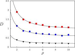
Figure 1: Diffusion coefficient $D$ as a function of the density of particles $\rho$ for a single species, calculated from simulation of the model for three different temperatures: $T=0.3$ (squares), $T=0.18$ (circles) and $T=0.06$ (triangles). Solid lines correspond to Eq. (5).

Note that at low temperatures the diffusion coefficient calculated from simulations agrees with the mesoscopic diffusion coefficient given by Eq. (5). These results show that multiparticle collision models can be used to simulate systems with relatively low temperatures ($T=0.06$), keeping a good diffusive behavior.

To implement the multiparticle-collision model with repulsion, Eqs. (1)-(4), we consider a three-dimensional film with length $L_{x}=100$ units along $x$, width $L_{y}=100$ units along $y$, and height $L_{z}=2$ units along $z$. We impose periodic boundary conditions in the $y$ and $z$ directions, and bounce-back reflection boundary conditions on both the left and the right side of the film along the $x$ direction. The average number of particles per cell is assumed to be the same for both species; i. e., $n^{A}=n^{B}\equiv n$. Additionally, we assume species with equal masses; i. e., $m^{A}=m^{B}\equiv m$.

First, we study the properties of the interface between the two fluids. As initial condition, particles of species $A$ are uniformly distributed at random on the right side of the film, so that their mean density, averaged over cells, is $\rho^{A}(x\geq 50)=2mn$ and $\rho^{A}(x<50)=0$; while particles of species $B$ are similarly distributed on the left side of the film; i.e., $\rho^{B}(x\leq 50)=2mn$ and $\rho^{B}(x>50)=0$.

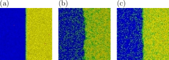
Figure 2: Snapshots along the $z$-axis of the system for $T=0.12$ and $\kappa=5$. Particles of species $A$ are assigned a yellow (light gray) color and particles of species $B$ are marked in blue (black). Green (dark gray) color indicates the presence of particles of both species. The color intensity is proportional to the density of particles. (a) Initial state. (b) State after $t=10^{5}$ iterations for $n=5$. (c) State after $t=10^{5}$ iterations for $n=8$.

Figure 2(a) shows a snapshot of the initial condition of the system. Figures 2(b) and 2(c) show snapshots of the system at $t=10^{5}$ iterations with parameters $n=5$ and $n=8$, respectively. Note that in both, Fig. 2(b) and Fig. 2(c), the system maintains two phases separated by a thin region where species $A$ and $B$ are mixed. That is, the multiparticle-collision repulsion model is able to stabilize the interface for some values of the parameters of the system.

To characterize the interface, we calculate the normalized density profile, defined as

$$\Delta\rho^{\gamma}(x)=\frac{\rho^{\gamma}(x)-\rho^{\gamma^{*}}(x)}{\rho^{\gamma}_{\infty}}\;,$$ (6)

where $\rho^{\gamma}(x)$ is the mean density of species $\gamma$ in cells with coordinate $x$, and $\rho^{\gamma}_{\infty}=2mn$ is the value of $\rho^{\gamma}(x)$ far from the interface.

Figure 3 shows the variation of the normalized density profile for two different number of particles per cell. Note that, as the number of particles per cell increases, the interface gets sharper. This effect is expected since the repulsion between particles of different species increases with the increment of their respective densities.

Figure 3: Variation of the normalized profile density $\Delta\rho^{\gamma}(x)$ as a function of $x$, for $n=5$ (open circles) and $n=8$ (solid circles), with fixed parameter values $T=0.12$, $\kappa=5.0$. The solid and dashed lines are the fittings of Eq. (7) for $n=5$ and $n=8$, respectively.

To measure the interface width, denoted by $\zeta$, we have fitted the simulation points in the interface profile of Fig. 3 with the function TSafran ,

$$\Delta\rho^{\gamma}(x)=\tanh{\left(\frac{x}{\zeta}\right)}.$$ (7)

The behavior of the interface width $\zeta$ as function of the repulsion parameter $\kappa$ is shown in Fig. 4. There is a critical value of $\kappa_{c}\approx 0.6$, above which $\zeta$ reaches an asymptotic minimum value. This indicates that repulsion between species due to collisions, represented in Eq. (4), becomes maximum for values $\kappa>\kappa_{c}$.

Figure 4: Mean interface width $\zeta$ as a function of the repulsion parameter $\kappa$ with fixed parameter values $n=5$ and $T=0.12$, after $t=10^{5}$ iterations.

The effect of the temperature on the interface width can be approximated by using the classical Ising model for an interface between two species TSafran ,

$$\zeta\sim\frac{1}{(T_{c}-T)^{1/2}}\;,$$ (8)

where $T_{c}$ is the critical temperature for the formation of the interface.

In Fig. 5 we compare the numerical results obtained from our model with the values given by Eq. (8), for two different values of $n$. There is good agreement between the behavior described by Eq. (8) and the simulations. The critical temperatures, calculated from the fitting of the numerical points to Eq. (8), are $T_{c}\approx 0.162$ for $n=5$ and $T_{c}\approx 0.173$ for $n=8$.

Figure 5: Mean interface width $\zeta$ as a function of the temperature $T$, for $n=5$ (solid circles) and $n=8$ (open circles) at $t=10^{5}$ iterations. Fixed parameter $\kappa=5$. Continuous lines correspond to Eq. (8).

Another property that characterizes an interface is the interfacial tension, denoted by $\Gamma$. A simple way to estimate $\Gamma$ is through the expression TSafran

$$\Gamma\sim\frac{4\,\rho^{\gamma}_{\infty}}{3\,\zeta}.$$ (9)

Figure 6 shows $\Gamma$, obtained from Eq. (9), as a function of temperature. The simulation points are compared with the theoretical expression for interfacial tension given by the Ising model TSafran ,

$$\Gamma\sim\frac{(T_{c}-T)^{3/2}}{T}.$$ (10)

Figure 6: Interface tension $\Gamma$ as a function of the temperature $T$ at $t=10^{4}$ iterations. Fixed parameter values are $\rho^{\gamma}_{0}=5$, $\kappa=5$.

Note that, for temperatures $T\geq 0.06$, the interfacial tension calculated from the simulations and Eq. (9) are well fitted by the the theoretical curve, Eq. (10).

It is known, from direct molecular dynamics simulations with two immiscible Lennard-Jones fluids DARF1 , as well as from density functional theory IF1 , that the interfacial tension $\Gamma$ exhibits a maximum as the the temperature is varied. The maximum value of $\Gamma$ arises at a temperature such the attractive interaction forces between particles cancel out the thermal effect. For temperatures above this point, the thermal effect is sufficiently strong to cause a decrease of the value of $\Gamma$. Our multiparticle collision binary fluid model agrees well with the behavior of $\Gamma$ predicted by the Ising model for temperatures at which the thermal effect is dominant. However, in the multiparticle collision binary fluid model, the attractive interaction forces between particles are not explicit, but they are represented by rotation operators.

Next, we consider the problem of phase separation of an immiscible binary fluid in the framework of our model. The dimensions of the sides of the box are $L_{x}=L_{y}=100$, and $L_{z}=2$, and we assume that the volume has periodic boundary conditions in all three axes. We start from homogeneous initial conditions where both species are uniformly distributed in the volume of the simulation box.

Figure 7 shows four snapshots of the evolution of the system. The initial well-mixed state is displayed in Fig. 7(a). Figures 7(b)-(d), for successive times, show the spontaneous formation of of a segregated state, where domains become separated by a thin interface.

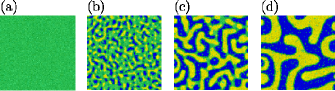
Figure 7: Snapshots along the $z$-axis of the patterns during the evolution of the system, with fixed parameter values $L_{x}=L_{y}=100$, $L_{z}=2$, $\rho^{\gamma}_{0}=5$, $T=0.09$ and $\kappa=5.0$. Particles of species $A$ are assigned a yellow (light gray) color and particles of species $B$ are marked in blue (black). Green (dark gray) color indicates the presence of particles of both species. The color intensity is proportional to the density of particles. a) Initial condition. b) $t=10^{2}$. c) $t=10^{3}$. d) $t=10^{4}$.

A domain growth can be characterized by the time evolution of the average radius, as

$$R_{t}\sim t^{\alpha}\;,$$ (11)

where $R_{t}$ is the average radius of the phase domain at time $t$, and $\alpha$ is the growth exponent. We define the average radius $R_{t}$ as the distance $r$ where the spatial correlation function $C[r,t]$ first becomes zero; that is,

$$R_{t}=\min\{r\,\forall\,C[r,t]\}=0.$$ (12)

The spatial correlation function using the discrete cells of the model can be calculated as

$$C[r,t]=\langle\Phi_{t}(\xi)\Phi_{t}(\xi^{\prime})\rangle_{\xi,\xi^{\prime}},$$ (13)

where $r=|{\bf r}_{\xi}-{\bf r}_{\xi^{\prime}}|$ is the distance between the center of cell $\xi$ and the center of cell $\xi^{\prime}$, $\langle\cdots\rangle_{\xi,\xi^{\prime}}$ is the spatial average over all pairs of cells $\xi$ and $\xi^{\prime}$ separated a distance $r$, and

$$\Phi_{t}(\xi)=\rho^{\gamma}_{t}(\xi)-\rho^{\gamma^{*}}_{t}(\xi)$$ (14)

is the difference between the densities of species $\gamma$ and $\gamma^{*}$ in the cell $\xi$ at time $t$.

Figure 8: Average radius of a domain phase $R_{t}$, shown as black dots, as a function of time $t$ in log-log scale. Fixed parameter values are $L_{x}=L_{y}=200$, $L_{z}=2$, $\rho_{0}^{\gamma}=5$, $T=0.09$ and $\kappa=5.0$. The continuous line corresponds to the best fitting of Eq. (11) for points in the interval $t\in[10^{2},10^{5}]$.

Figure 8 shows $R_{t}$ as a function of time, in a log-log plot, with a fixed temperature. The logarithm of the radius $R_{t}$ increases linearly with the logarithm of time in the interval $t\in[10^{2},10^{5}]$. The corresponding slope, obtained by fitting of the data, yields the growth exponent $\alpha\approx 0.37$, which is close to the theoretical value for phase growth in a diffusive regime TSafran . For times greater than $t=10^{5}$, the domain size reaches half of the size of the simulation box; that is, $R_{t}\approx L_{x}/4$, and the domain growth slows down.

Figure 9 shows the growth exponent $\alpha$ as a function of the temperature $T$, calculated numerically from data in the time interval for which Eq. (11) is valid. The exponent $\alpha$ decays linearly with increasing temperature up to a value $T\approx 0.2$. Above this critical temperature, the error bars in the determination of the quantity $\alpha$ are too large, and the interface becomes unstable because the thermal mixing destroys the phase separation process.

Figure 9: Growth exponent $\alpha$ as a function of temperature $T$. Fixed parameter values are $L_{x}=L_{y}=100$, $L_{z}=2$, $\rho=5$ and $\kappa=5.0$. Error bars represent the standard error of the fit of Eq. (11).

IV Binary fluid in crowded environment

The motion of fluids in crowded environment by obstacles is a problem of much interest in cell biology and other contexts Zhou ; Verkman ; Loren . One way of modeling a film of fluid in a crowded environment is by placing a set of cylindrical obstacles in the system EK1 . To simulate the behavior of a binary fluid in a crowded environment with our model, we insert $N_{S}$ stationary cylinders in a volume of radius $\sigma$ and height equal to the height of the simulation box $L_{z}$. The fraction of volume occupied by the obstacles is $\phi=2\pi N_{S}\sigma^{2}L_{z}/{\cal V}$. We fix the radius of the cylinders at the value $\sigma=2.5$ in units of cells.

As in the previous simulations, particles of one species are distributed uniformly in the right half-side of the simulation box while particles of the other species are distributed on the left half-side of the box. We set the particles velocities using a Boltzmann distribution with temperature $T$, and fix the densities $\rho=\rho^{\gamma}=\rho^{\gamma*}=5$ and the repulsion parameter at the value $\kappa=5$. We assume that, when a particle of either species collides with an obstacle, its velocity is reversed, i.e., a bounce back collision occurs.

Figure 10 shows two snapshots of the system when the interface has stabilized, for different values of the fraction of volume occupied by obstacles. Note that the interface lies close to obstacles and looks distorted. This effect is consequence of the reduction of pressure that occurs when the distance between the interface curve and an obstacle is small enough to produce an imbalance of forces that removes the particles lying between the interface and the obstacle.

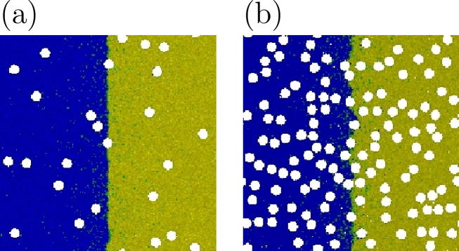
Figure 10: Snapshots along the $z$-axis of the system forming a stable interface at $t=10^{4}$ iterations, for different values of the volume fraction of obstacles $\phi$. White circles indicate the cylindrical obstacles. Fixed parameters are $\rho=5$, $\kappa=5.0$ and $T=0.06$. (a) $\phi=0.05$. (b) $\phi=0.25$.

We also study the phenomenon of spontaneous phase separation of an immiscible binary fluid in a crowded environment. In this case, the particles of each species are initially distributed uniformly throughout the volume of the simulation box, avoiding the space occupied by the obstacles.

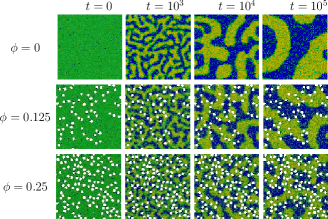
Figure 11: Snapshots along the $z$-axis of the evolution of the phase growth for three different values of the volume fraction, $\phi=0.0$, $0.125$ and $0.25$ (from top to bottom) and for four different times $t=0$, $10^{3}$, $10^{4}$ and $10^{5}$ (from left to right). White circles indicate the cylindrical obstacles. Fixed parameter values are $\rho^{\gamma}=\rho^{\gamma*}=5$, $\kappa=5.0$ and $T=0.09$.

Figure 11 shows the snapshots of the evolution of phase growth processes for three different values of the volume fraction of obstacles $\phi$. As expected, the phase growth process from a homogeneous state is affected by the presence of obstacles. At first glance, we can see that growth becomes slower when $\phi$ is increased, since obstacles impede the aggregation of particles in domains. Additionally, we see that the interfaces lie along the locations of obstacles, lacking the rounded profile that they possess when the media is free.

To investigate the effect of obstacles on the phase growth process, we have calculated the time evolution of the average radius of the phase domain $R_{t}$ for several values of $\phi$, as shown in Fig. 12(a). For each value of $\phi$, $R_{t}$ can be adjusted to the expression Eq. (11) in the time interval $t\in[10^{2},10^{5}]$. This allows to calculate the growth exponent $\alpha$ as a function of $\phi$, as shown in Fig. 12(b). We can see that increasing the density of obstacles leads to a decrease in the velocity of the phase growth process, represented by the exponent $\alpha$.

     

Figure 12: (a) Average radius of the phase domain $R_{t}$ as function of time $t$ in the presence of obstacles, in log-log scale for $\phi=0.0$ ($\circ$), $\phi=0.125$ ($\triangle$) and $\phi=0.25$ ($\square$). (b) Growth exponent $\alpha$ as function of $\phi$ in the presence of obstacles. Fixed parameter values are $L_{x}=L_{y}=50$, $L_{z}=2$, $\rho^{\gamma}=\rho^{\gamma*}=5$, $T=0.09$ and $\kappa=5.0$. Error bars represent the standard error of the fit of Eq. (11).

V Conclusions

We have proposed a multiparticle collision dynamics model to investigate phase separation processes in a binary fluid. To this aim, we have introduced a repulsion rule between the centers of mass of particles from different species to simulate segregation in a binary fluid. We have applied this model to mesoscopic systems in both free and crowded environments, where the volume has been discretized into finite cells.

Since the repulsion rule only depends on the configuration of the particles inside each cell, the model maintains Galilean invariance. In addition, the multiparticle-collision model with repulsion conserves the mass and the energy of the system at micro and macro scales, while momentum is conserved within homogeneous domains, but not at the interfaces.

In spite of this limitation, the multiparticle-collision repulsion model yields results consistent with the known behavior of binary fluids. Properties such as diffusion coefficient, density profile and width of the interface, calculated from simulations of the multiparticle-collision repulsion model, agree very well with the theoretical values predicted by the Ising model for interfaces in a wide range of temperatures and densities. For moderately and low temperatures, the model is able to simulate the segregation of an immiscible binary fluid into domains, starting from mixed, homogeneous initial conditions. Moreover, the growth exponents for the phases obtained from the model are similar to the corresponding growth exponents that characterize Newtonian binary fluids.

We have extended the multiparticle-collision repulsion model to simulate crowded environments. The results from the simulations are also consistent with the behavior of binary fluids in these environments.

The good performance of the multiparticle-collision repulsion model for a binary fluid suggests that it can be generalized to incorporate other phenomena, such as chemical reactions among the species, and to consider species that may diffuse at different rates. In addition, because of its low computational cost, the multiparticle-collision repulsion model can be used to simulate systems with relatively large scales of time and space; i.e., simulate systems with millions of particles per millions of iterations.

References

- (1) Müller M., Charypar D., Gross M. Particle-based fluid simulation for interactive applications. In Proceedings of the 2003 ACM SIGGRAPH/Eurographics symposium on Computer animation 2003;154-159.
- (2) Premžoe S, Tasdizen T, Bigler J, Lefohn A, Whitaker, RT. Particle‐Based Simulation of Fluids. In Computer Graphics Forum. 2003;22:401-410.
- (3) Mills, Zachary Grant and Mao, Wenbin and Alexeev, Alexander, Mesoscale modeling: solving complex flows in biology and biotechnology, Trends in Biotechnology 31, 426 (2013).
- (4) Saunders, Marissa G and Voth, Gregory A, Coarse-graining methods for computational biology, Annual Review of Biophysics, 42, 73 (2013).
- (5) Frisch U, Hasslacher B, Pomeau Y. Lattice-Gas Automata for the Navier-Stokes Equation, Phys. Rev. Lett., 1986;56:1505-1508.
- (6) Succi S, The Lattice Boltzmann Equation for Fluid Dynamics and Beyond. Oxford University Press, Oxford (2001).
- (7) Hoogerbrugge PJ, Koelman J. Simulating Microscopic Hydrodynamic Phenomena with Dissipative Particle Dynamics. Europhys. Lett. 1992;19:155-160.
- (8) Groot RD, Warren PB. Dissipative particle dynamics: Bridging the gap between atomistic and mesoscopic simulation. J. Chem. Phys. 1997;107:4423-4435.
- (9) Español P, Revenga M. Smoothed dissipative particle dynamics. Phys. Rev. E, 2003;67:026705-026705.
- (10) Malevanets A, Kapral R. Mesoscopic model for solvent dynamics. J. Chem. Phys. 1999;110:8605-8613.
- (11) Malevanets A, Kapral R. Solute molecular dynamics in a mesoscale solvent. J. Chem. Phys. 2000;112:7260-7269.
- (12) Malevanets A, Kapral R. Mesoscopic multi-particle collision model for fluid flow and molecular dynamics Novel Methods in Soft Matter Simulations. ed. M Karttunen, I. Vattulainen and A. Lukkarinen (Berlin: Springer). 2003.
- (13) Gompper G, Ihle T, Kroll K, Winkler RG. Multi-Particle Collision Dynamics: A Particle-Based Mesoscale Simulation Approach to the Hydrodynamics of Complex Fluids, Advanced Computer Simulation Approaches for Soft Matter Sciences III, Advances in Polymer Science. 2009;221:1-87.
- (14) Padding J T, Louis AA. Hydrodynamic and Brownian Fluctuations in Sedimenting Suspensions. Physical Review Letters. 2004;93:220601-220605.
- (15) Hecht M, Harting J, Bier M, Reinshagen J, Herrmann HJ. Shear viscosity of claylike colloids in computer simulations and experiments. Physical Review E. 2006;74:021403-021418.
- (16) Mussawisade K, Ripoll M, Winkler RG, Gompperand G. Dynamics of polymers in a particle-based mesoscopic solvent. Journal of Chemical Physics. 2005;123:144905-144916.
- (17) Ripoll M, Winkler RG, Gompperand G. Hydrodynamic screening of star polymers in shear flow. The European Physics Journal E. 2007;23:349-354.
- (18) Echeverria C, Kapral R. Macromolecular Dynamics in Crowded Environments. J. Chem. Phys. 2010;123:104902-104913.
- (19) Echeverria C, Togashi Y, Mikhailov AS, Kapral R. A mesoscopic model for protein enzymatic dynamics in solution. Phys. Chem. Chem. Phys. 2011;13:10527-10537.
- (20) Echeverria C, Kapral R. Molecular crowding and protein enzymatic dynamics. Phys. Chem. Chem. Phys. 2012;14:6755-6763.
- (21) Echeverria C, Kapral R. Diffusional correlations among multiple active sites in a single enzyme. Phys. Chem. Chem. Phys. 2014;15:6211-6216.
- (22) Noguchi H, Gompper G. Dynamics of fluid vesicles in shear flow: Effect of membrane viscosity and thermal fluctuations, Physical Review E. 2005;72:011901-011915.
- (23) Rohlf K, Fraser S, Kapral R. Reactive multiparticle collision dynamics. Computer Physics Communications. 2008;179:132-139.
- (24) Tucci K, Kapral R. Mesoscopic model for diffusion-influenced reaction dynamics. J. Chem. Phys. 2004;120:8262–8271.
- (25) Tucci K, Kapral R. Mesoscopic Multiparticle Collision Dynamics of Reaction−Diffusion Fronts. J. Phys. Chem. B. 2005;109:21300-21304.
- (26) Echeveria C, Tucci K, Kapral R. Diffusion and reaction in crowded environments. J. Phys.: Condens. Matter, 2007;19:065146-065158.
- (27) Echeverria C, Kapral R. Autocatalytic reaction dynamics in systems crowded by catalytic obstacles. Physica D. 2010;239:791-796.
- (28) Hashimoto Y, Chen Y, Ohashi H. Immiscible real-coded lattice gas. Comp. Phys. Comm. 2000;56:56-62.
- (29) Inoue Y, Chen Y, Ohashi H. A mesoscopic simulation model for immiscible multiphase fluids. Journal of Computational Physics. 2004;192:191-203.
- (30) Sakai T, Chen Y, Ohashi and H. Real-coded lattice gas model for ternary amphiphilic fluids. Phys. Rev. E, 2002;65:031503-031511.
- (31) Drube F. Selfdiffusiophoretic Janus Colloids. Doctoral dissertation, Ludwig-Maximilians-Universität, München, 2013.
- (32) Tüzel E, Pan G, Ihle T, Kroll DM. Mesoscopic model for the fluctuating hydrodynamics of binary and ternary mixtures, Europhysics Letters, 2007;80:40010-40017.
- (33) T. Ihle, D.M. Kroll, Stochastic rotation dynamics: A Galilean-invariant mesoscopic model for fluid flow. Phys. Rev. E, 63 (2001) 020201–020205.
- (34) Laradji M, Toxvaerd S, Mouritsen OG. Molecular Dynamics Simulation of Spinodal Decomposition in Three-Dimensional Binary Fluids. Phys. Rev. Lett. 1996;77:2253-2257.
- (35) Samual A. Safram, Statistical Thermodynamics of Surfaces. Interfaces and Membranes. Addison-Wesley; 1994.
- (36) Diaz-Herrera E, Alejandre J, Ramirez-Santiago G, Forstmann F. Interfacial tension behavior of binary and ternary mixtures of partially miscible Lennard-Jones fluids: A molecular dynamics simulation. J. Chem. Phys. 1999;110:8084-8091.
- (37) Iatsevitch S, Forstmann F. Density profiles at liquid-vapor and liquid-liquid interfaces: An integral equation study. J. Chem. Phys. 1997;107:6925-6935.
- (38) Zhou HX, Rivas G, Minton AP. Macromolecular crowding and confinement: biochemical, biophysical, and potential physiological consequences. Annu Rev Biophys. 2008;37:375-397.
- (39) Verkman AS. Solute and macromolecule diffusion in cellular aqueous compartments. Trends Biochem Sci. 2002;27:27-33.
- (40) Loren S, Shao-Qing Z, Margaret SC, Pernilla Wittung-Stafshede. Molecular crowding enhances native structure and stability of protein flavodoxin, Proc Natl Acad Sci U S A. 2007;104:18976-18981.