Relatively recently (A. Amaya-Tapia, S. Y. Larsen, M. Lassaut. Ann. Phys.,306 (2011) 406), we presented a formula for the evaluation of the third Bose fugacity coefficient - leading to the third virial coefficient - in terms of three-body eigenphase shifts, for particles subject to repulsive forces. An analytical calculation for a 1-dim. model, for which the result is known, confirmed the validity of this approach. We now extend the formalism to particles with attractive forces, and therefore must allow for the possibility that the particles have bound states. We thus obtain a true generalization of the famous formula of Uhlenbeck and Beth (G.E. Uhlenbeck, E. Beth. Physica,3 (1936) 729; E. Beth, G.E. Uhlenbeck. ibid, 4 (1937) 915) (and of Gropper (L. Gropper. Phys. Rev. 50 (1936) 963; ibid 51 (1937) 1108)) for the second virial. We illustrate our formalism by a calculation, in an adiabatic approximation, of the third cluster in one dimension, using McGuire’s model as in our previous paper, but with attractive forces. The inclusion of three-body bound states is trivial; taking into account states having asymptotically two particles bound, and one free, is not.

Introduction

Our goal, over many decades, has been to develop a generalization of the formula of Uhlenbeck and Beth[1](and also of Gropper[2]), which yields the second virial in terms of phase shifts and bound state energies. This would be an expression for the higher virials, in terms of quantities which characterize the asymptotic - long range - behaviour of the wave functions which appear in an eigenfunction evaluation of the Statistical Mechanical traces. These would be eigenphase shifts and bound state energies.

This effort has led to an approach for the third virial using an expansion of the wave functions in terms of hyperspherical harmonics[3] - only made really useful by an adiabatic approximation. Among other results, one has been able to show that in the semi-classical limit, for repulsive forces, one recovers the known classical results from an eigenphase shift formulation[4]. See, also, the calculation of the third virial in two dimensions, for repulsive step potentials[5, 6, 7], and - as a bonus but important - a formulation of the second virial for particles subject to anisotropic forces[8], i.e., for a Helium atom and a Hydrogen molecule.

This latter formulation, in fact, has been crucial for us. It showed how, instead of putting particles in a box and calculating a density of states, one could use a procedure similar to that used in obtaining a Wronskian, and obtain analytically the result of integrating the square of the wave functions, in terms of these wave functions (and their derivatives) at the origin (giving zero) and at the long range limit of integration. I.e., it permitted us to work in the continuum and to express our results in terms of asymptotic quantities, precisely eigenphase shifts and bound state eigenvalues.

The next crucial step, for our three particles, towards including the bound states - such as having the possibility at long range of a 2 body bound state and a free particle - was to take advantage of a hyperspherical adiabatic basis[9].

Its importance is two-fold.

The first is due to the fact that, even for short ranged 2-body potentials, the effective few-body interactions are long ranged and so, also, are their effects on the continuum wave functions. The use of the hyperspherical adiabatic basis, which incorporates information valid for large values of the hyper radius, is tremendously helpful.

The second is that at large distances the free and bound structures are made explicitly clear[10] and, in an expansion, are associated with distinct amplitudes.

We note, for example, that in a three-body problem with a 2-body bound state, at least one of the elements of the adiabatic basis will have, built in, the cluster property of the 2 bodies, and others will correspond to asymptotically free particles.

We note also that in both hyperspherical approaches the hard step conceptually is to pass from two to three particles. The extension to a higher number of particles is straightforward. We limit ourselves here to a maximum of three particles, sufficient for the third virial.

In a hyperspherical adiabatic reformulation of our formalism, we were then able, in the absence of bound states, to give a formula expressing the quantum mechanical third cluster, in terms of adiabatic phase shifts[9]. (This for Boltzmann statistics.) From this q. m. formalism, under the same constraints, we were again able to recover, as $\hbar$ goes to $0$, the classical expression. We also discussed some of the difficulties that arise in the presence of 2-body bound states and presented a tentative formula involving eigenphase shifts and 2 and 3 body bound state energies.

Recently, we generalized our formalism to accommodate Bose statistics and calculated[11] the third fugacity coefficient for a version of a model due to McGuire[12]. It consists of 3 particles on a line, subject to repulsive delta function potentials. The model allowed us to obtain many results in analytical form[13, 14] and to compare our results with those of Dodd and Gibbs[15], who integrated expressions requiring the complete (known) wave functions for this model. This confirmed the validity of our (more general) approach.

In the present work, we return to the problem of the bound states. It simplifies our discussion to use particles subject to quantum statistics (say Bose) and though our formalism is stated for three dimensions, we will illustrate the behaviour of certain potentials and bound state situations by borrowing results from our previous work in one dimension. In addition we present new results for McGuire’s model, this time yielding the virial for attractive potentials.

We will see that in the complete generalization, we still encounter certain difficulties and constraints and we discuss subtleties and fine points in the whole attempt to establish phase shifts plus bound state formalisms - even for the second virial.

Statistical Mechanics

We start with the Grand Partition function:

$${\cal Q}={\displaystyle\sum_{n=0}^{\infty}z^{n}{}Tr\left(e^{-\beta H_{n}}\right)}=1+zTr\left(e^{-\beta T_{1}}\right)+z^{2}{}Tr\left(e^{-\beta H_{2}}\right)+z^{3}{}Tr\left(e^{-\beta H_{3}}\right)+\cdots$$ (1)

The fugacity $z$ equals $\exp\left(\mu/\kappa T\right)$;$\;\beta=1/\kappa T$, where $\mu$, $\kappa$ and $T$ are the Gibbs’ function per particle, Boltzmann’s constant and the temperature, respectively. $H_{n}$ and $T_{n}$ are the n-particle Hamiltonian and kinetic energy operators.

We note that no factor of ($1/n!$) appears in this development. This is correct for Bose or Fermi statistics. Also important, is the fact that

$$Tr\left(e^{-\beta H_{n}}\right)\rightarrow V^{n}\;\;{\rm as}\;{\rm the}\;{\rm volume}\;\;V\;\rightarrow\;{\rm large},$$

leading to the divergence of the individual traces in the thermodynamic limit. If we take, however, the logarithm of the Grand Partition function ${\cal Q}$, we obtain

$$\begin{array}[]{cl}ln{\cal Q}&=z\,\,Tr\left(e^{-\beta T_{1}}\right)\\ &+z^{2}\left[Tr\left(e^{-\beta H_{2}}\right)-\frac{1}{2}\left[Tr\left(e^{-\beta T_{1}}\right)\right]^{2}\right]\\ &+z^{3}\left[Tr\left(e^{-\beta H_{3}}\right)-Tr\left(e^{-\beta T_{1}}\right)Tr\left(e^{-\beta H_{2}}\right)+\frac{1}{3}\left[Tr\left(e^{-\beta T_{1}}\right)\right]^{3}\right]\\ &+\cdots\end{array}$$ (2)

which, when divided by V, gives coefficients of the powers of $z$, which are independent of the volume, when the latter becomes large. They are the fugacity coefficients $b_{l}$. We can then write for the pressure and the density

$$p/\kappa T=(1/V)\ln{\cal Q}=\sum_{l}b_{l}\,z^{l},$$

$$N/V=\rho=\sum_{l}l\,b_{l}\,z^{l},$$

and the fugacity can be eliminated to yield the pressure in terms of the density, in the virial expansion:

$$\frac{p}{\mathrm{k}T}=\sum_{n=1}^{\infty}B_{n}\rho^{n}.$$

The third fugacity coefficient, Bose statistics

From Eq.(2), an expression for the 3rd fugacity coefficient can be written as

$$b_{3}=\frac{1}{V}\left[Tr\left(e^{-\beta H_{3}}\right)-Tr\left(e^{-\beta T_{1}}\right)Tr\left(e^{-\beta H_{2}}\right)+\frac{1}{3}Tr\left(e^{-\beta T_{1}}\right)^{3}\right]$$ (3)

Note that each of the 3 terms in the bracket, above, grows as $V^{3}$ asymptotically, for large $V$. Therefore, subtractions must take place, so that $b_{3}$ might become independent of $V$, as is required. If we factor out the contribution of the C.M. (proportional to $V$), each term will have a dependence proportional to $V^{2}$.

To help us decrease the $V$ dependence, let us subtract, from each of terms above, the equivalent term without interaction. Subtracting, therefore, $b_{3}^{0}$ from the $b_{3}$, we obtain:

$$b_{3}-b_{3}^{0}=\frac{1}{V}\left[Tr\left(e^{-\beta H_{3}}-e^{-\beta T_{3}}\right)-Tr\left(e^{-\beta T_{1}}\right)Tr\left(e^{-\beta H_{2}}-e^{-\beta T_{2}}\right)\right].$$ (4)

For Boltzmann statistics $b^{0}_{3}$ equals zero. For Fermi and Bose statistics $b^{0}_{3}=1/(3^{5/2}\lambda^{3}_{T})$, where $\lambda^{3}_{T}=(2\pi\hbar^{2}\beta/m)^{3/2}$, and $\lambda_{T}$ is the thermal wave length. We have ignored the factors associated with spin.

To subtract volumes from comparable volumes, we rewrite the traces so that the arguments of the exponentials are all 3-body Hamiltonians:

$$b_{3}-b_{3}^{0}=\frac{1}{V}\left[Tr\left(e^{-\beta H_{3}}-e^{-\beta T_{3}}\right)-Tr\left(e^{-\beta(H_{2}+T_{1})}-e^{-\beta(T_{2}+T_{1})}\right)\right].$$ (5)

One remark: We will evaluate the traces by inserting complete sets of states into the traces. For the terms involving $H_{3}$ and $T_{3}$, we will choose states having complete symmetry between the three particles. For the terms involving $H_{2}$ or $T_{2}$, above, we will need symmetry between say particles 1 and 2, with particle 3 acting as a spectator. The adiabatic functions that we define in the next section will have to satisfy these requirements. Different sets of indices will also be associated with each type of symmetry.

Hyperspherical Adiabatic Preliminaries

For the 3 particles of equal masses, in three dimensions, we first introduce center of mass and Jacobi coordinates. We define

$$\vec{\eta}=\left(\frac{1}{2}\right)^{1/2}(\vec{r}_{1}-\vec{r}_{2})\hskip 28.45274pt\vec{\xi}=\left(\frac{2}{3}\right)^{1/2}\left(\frac{\vec{r}_{1}+\vec{r}_{2}}{2}-\vec{r}_{3}\right)\hskip 28.45274pt\vec{R}=\,\;\frac{1}{3}\;(\vec{r}_{1}+\vec{r}_{2}+\vec{r}_{3})$$ (6)

Figure 1: Jacobi coordinates

where, of course, the $\vec{r}_{i}$ give us the locations of the 3 particles. This is a canonical transformation and insures that in the kinetic energy there are no cross terms.

The variables $\vec{\xi}$ and $\vec{\eta}$ are involved separately in the Laplacians and we may consider them as acting in different spaces. We introduce a higher dimensional vector $\vec{\rho}=(\begin{array}[]{c}\vec{\xi}\\ \vec{\eta}\end{array})$ and express it in a hyperspherical coordinate system ($\rho$ and the set of angles $\Omega$). If we factor a term of $\rho^{5/2}$ from the solution of the relative Schrödinger equation, i.e. we let $\psi=\phi/\rho^{5/2}$, we are led to:

$$\left[-\frac{\partial^{2}}{\partial\rho^{2}}+H_{\rho}-\frac{2mE}{\hbar^{2}}\right]\phi(k,\rho,\Omega)=0,$$ (7)

where

$$H_{\rho}=-\frac{1}{\rho^{2}}\left[\nabla^{2}_{\Omega}-\frac{15}{4}\right]+\frac{2m}{\hbar^{2}}V(\rho,\Omega),$$ (8)

$m$ is the mass of each particle, $E$ is the relative energy in the center of mass and $k^{2}$ is the relative energy multiplied by $2m/\hbar^{2}$. $\nabla^{2}_{\Omega}$ is the purely angular part of the Laplacian.

We now introduce the adiabatic basis, which consists of the eigenfunctions of part of the Hamiltonian: the angular part of the kinetic energy and the potential :

$$H_{\rho}B_{\ell}(\rho,\Omega)=\Lambda_{\ell}(\rho)B_{\ell}(\rho,\Omega),$$ (9)

where $\ell$ enumerates the solutions.

Using this adiabatic basis, we can now rewrite the Schrödinger equation as a system of coupled ordinary differential equations.

We write

$$\phi(k,\rho,\Omega)=\sum_{\ell^{\prime}}B_{\ell^{\prime}}(\rho,\Omega)\,\tilde{\phi}_{\ell^{\prime}}(k,\rho)$$ (10)

and obtain the set of coupled equations

$$\left(\frac{d^{2}}{d\rho^{2}}-\Lambda_{\ell}(\rho)+k^{2}\right)\,\tilde{\phi}_{\ell}(k,\rho)+2\sum_{\ell^{\prime}}C_{\ell,\ell^{\prime}}\,\frac{d}{d\rho}\,\tilde{\phi}_{\ell^{\prime}}(k,\rho)+\sum_{\ell^{\prime}}D_{\ell,\ell^{\prime}}\,\tilde{\phi}_{\ell^{\prime}}(k,\rho)=0,$$ (11)

where we defined:

$$C_{\ell,\ell^{\prime}}(\rho)=\int d\Omega\,B^{\ast}_{\ell}(\Omega,\rho)\frac{\partial}{\partial\rho}B_{\ell^{\prime}}(\Omega,\rho)\hskip 14.22636ptD_{\ell,\ell^{\prime}}(\rho)=\int d\Omega\,B^{\ast}_{\ell}(\Omega,\rho)\frac{\partial^{2}}{\partial\rho^{2}}B_{\ell^{\prime}}(\Omega,\rho).\$$ (12)

We note that

$$D_{\ell,\ell^{\prime}}=\frac{d}{d\rho}\left(C_{\ell,\ell^{\prime}}\right)+\left(C^{2}\right)_{\ell,\ell^{\prime}},$$ (13)

and that $C$ is antisymmetric and $C^{2}$ is symmetric.

Without Bound States

Let us first keep things as simple as possible. When there are no bound states, we may write for the relative part of the 3-body trace:

$$Tr(e^{-\beta H_{3}})=\int\!\!d\vec{\rho}\int\!\!dk\sum_{i}\psi^{i}(k,\vec{\rho})(\psi^{i}(k,\vec{\rho}))^{\ast}\;e^{-\beta(\frac{\hbar^{2}}{2m}k^{2})}\,,$$ (14)

where we have introduced a complete set of continuum eigenfunctions. Expanding in the adiabatic basis, we obtain

$$Tr(e^{-\beta H_{3}})=\int\!\!d{\rho}\int\!\!dk\sum_{i,\ell}|\tilde{\phi}^{i}_{\ell}(k,\rho)|^{2}\;e^{-\beta(\frac{\hbar^{2}}{2m}k^{2})},$$ (15)

where we note that we have integrated over the angles and taken advantage of the orthogonality of our $B_{l}$’s. We integrate from $0$ to $\infty$.

We now return to our expression for $b_{3}-b^{0}_{3}$ and proceed as above, drop the tildes (also in the subsequent equations), to obtain:

$$\frac{3^{3/2}}{\lambda_{T}^{3}}\int\!\!dk\,e^{-\beta E_{k}}\int\!\!d{\rho}\sum_{i,\ell}[(|{\phi}^{i}_{\ell}|^{2}-|{\phi}^{i}_{\ell,0}|^{2})-(|\bar{\phi}^{i}_{\ell}|^{2}-|\bar{\phi}^{i}_{\ell,0}|^{2})],$$ (16)

where we have evaluated the trace corresponding to the center of mass. The amplitudes ${\phi}^{i}_{\ell}$ correspond to $H_{3}$, $\bar{\phi}^{i}_{\ell}$ to $H_{2}+T_{1}$ and amplitudes with a zero belong to the free particles. We now make use of a Wronskian type procedure to evaluate the $\rho$ integrals. We first write

$$\int_{0}^{\rho_{max}}\!\sum_{\ell}|\phi^{i}_{\ell}(k,\rho)|^{2}\;d\rho=\lim_{k^{\prime}\rightarrow k}\int_{0}^{\rho_{max}}\!\sum_{\ell}\phi^{i}_{\ell}(k,\rho)\phi^{i}_{\ell}(k^{\prime},\rho)\,d\rho$$ (17)

and then, there is the procedure:

$$\int_{0}^{\rho_{max}}\!\sum_{\ell}\;(\!\! \!\phi^{i}_{\ell}(k,\rho) \!\!\phi^{i}_{\ell}(k^{\prime},\rho))d\rho=$$

$$\frac{1}{k^{2}-(k^{\prime})^{2}}\sum_{\ell}\;[\! \!\!\phi^{i}_{\ell}(k,\rho) \!\!\frac{d}{d\rho}\phi^{i}_{\ell}(k^{\prime},\rho)-\phi^{i}_{\ell}(k^{\prime},\rho)\frac{d}{d\rho}\phi^{i}_{\ell}(k,\rho)],$$ (18)

evaluated at $\rho=\rho_{max}$.
—————————————————————-
I.e. our identity is (see Appendix B):

$$\ \sum_{\ell}\frac{d}{d\rho}\left[\phi_{\ell}(k^{\prime},\rho)\frac{d}{d\rho}\phi_{\ell}(k,\rho)-\phi_{\ell}(k,\rho)\frac{d}{d\rho}\phi_{\ell}(k^{\prime},\rho)\right]$$

$$+\left(k^{2}-(k^{\prime})^{2}\right)\sum_{\ell}\phi_{\ell}(k,\rho)\ \phi_{\ell}(k^{\prime},\rho)$$

$$+2\ \sum_{\ell,{\ell}^{\prime}}\frac{d}{d\rho}\left[\phi_{\ell}(k^{\prime},\rho)\ C_{\ell,{\ell}^{\prime}}\ \phi_{{\ell}^{\prime}}(k,\rho)\right]=0$$ (19)

and we integrate with respect to $\rho$. Using then the fact that $\phi$ goes to zero, as $\rho$ itself goes to zero, and that C decreases fast enough for $\rho$ large, we are left with the expression displayed earlier.
—————————————————————-
We now put in the asymptotic form of our oscillatory solutions, valid for $\rho_{max}$ sufficiently large, given the set of $\ell$’s, and use l’Hospital’s rule to take the limit as $k^{\prime}\rightarrow k$.
The solutions are:

$$\phi^{i}_{\ell}(k,\rho)\rightarrow(k\rho)^{1/2}\,{\cal C}_{\ell}^{i}(k)\,[\cos\delta^{i}(k)\>J_{K+2}(k\rho)-\sin\delta^{i}(k)\>N_{K+2}(k\rho)]$$ (20)

where the order $K$ is one of the quantities specified by $\ell$.

Obviously this requires comment. We show, in Appendix A, how given N coupled equations, we can choose the solutions so as to diagonalize a matrix W, analogous to an R-matrix, but characterising adiabatic solutions. These might be called ‘eigenstates of the standing waves’.

These will have the property that, for each solution, a unique eigenphase shift will appear in all of the associated amplitudes. Further, in the asymptotic regime, the adiabatic functions $B_{\ell}$, will - in the absence of interaction - reduce to hyperspherical harmonics, characterized, in part, by the order $K$. This, in turn implies that in the asymptotic form for the amplitude, there appears a term ${K+2}$.

The $\cal{C}$ is the coefficient of mixture, which tells us how much of each amplitude appears in each solution. Of course, we choose orthonormal eigenfunctions.

Inserting (20) into our integrals we find that

$$\sum_{\ell}\int_{0}^{\rho_{max}}\!|\phi^{i}_{\ell}(k,\rho)|^{2}\>d\rho\rightarrow\frac{1}{\pi}\frac{d}{dk}\delta^{i}(k)+\frac{1}{\pi}\rho_{max}\>+\>osc.\>terms$$ (21)

and, thus, that

$$\int_{0}^{\rho_{max}}\!(|\phi^{i}_{\ell}(k,\rho)|^{2}-|\phi^{i}_{\ell,0}(k,\rho)|^{2})\;d\rho\rightarrow\frac{1}{\pi}\frac{d}{dk}\delta^{i}(k)\>+\>osc.\>terms$$ (22)

We let $\rho_{max}$ go to infinity, and the oscillatory terms - of the form $\sin(2k\rho_{max}+\cdots)$ - will not contribute to the subsequent integration over $k$. [This is in 3 dimensions. In one dimension, we have shown that even for the second virial coefficient[16], the oscillatory terms can give a contribution.] Our basic formula now reads:

$$b_{3}-b^{0}_{3}\,=\,\frac{3^{3/2}}{\pi\lambda^{3}_{T}}\int_{0}^{\infty}\!dk\;\frac{d}{dk}\,G(k)\;e^{-\beta\frac{\hbar^{2}}{2m}k^{2}}$$ (23)

where

$$G(k)=\sum_{i}\>\delta^{i}(k)-\sum_{j}\>\bar{\delta}^{j}(k)$$ (24)

The first $\delta^{\prime}s$ arise from comparing three interacting particles with three free particles. The second $\bar{\delta^{\prime}s}$ arise when a 3-body system, where only two particles are interacting (one particle being a spectator), is compared to three free particles.

The evaluation of these sums (and their difference) is a delicate matter. The individual sums are separately infinite, as they correspond, classically to parts of the three-body cluster which depend on the volume. It is crucial to subtract individual, respective terms - before summing - to obtain a finite result.

We also observe that, if we limit ourselves to a finite number of the coupled equations, there will be fewer of the $\delta^{\prime}s$ than of the $\bar{\delta^{\prime}s}$, due to the requirements of symmetry, but that the $\delta^{\prime}s$ will, in their totality, be as important as the $\bar{\delta^{\prime}s}$ because they are associated with 3 binary potentials, while the $\bar{\delta^{\prime}s}$ will only reflect the potential of a pair.

Bound States

Of course, we shall need again to evaluate the relative part of the Bose trace:

$$Tr[(e^{-\beta H_{3}}-e^{-\beta T_{3}})-\,(e^{-\beta(H_{2}+T_{1})}-e^{-\beta(T_{2}+T_{1})})]$$ (25)

We shall have to discuss the contribution of each of the terms above but (as before) only integrating over a radius $\rho$ extending to an appropriately large value of $\rho_{max}$. The terms in $\rho_{max}$ must cancel.

If there are bound states, the major change in the eigenpotentials, see Eqs. (9, 11), is that for some of these potentials, the $\Lambda^{\prime}s$, instead of going to zero at large distances (large $\rho$), tend to a negative ‘plateau’. I.e., the eigenpotentials become flat and negative. We illustrate this with an example from our work in one dimension, with attractive delta-function potentials[17].

Here we present, illustrate, the dominant diagonal part of the adiabatic coupling matrix for the first few equations. In Fig. 2, we plot the first few even eigenvalues $\Lambda_{K}$ (with $K=0,6,12,...$) as a function of $\rho$.

Figure 2: Adiabatic eigenvalues $\Lambda_{K}$ for $c=-1$ (see Eq. 46). The points represent the two-body bound state energy level at $-\pi^{2}/36$

.

The plateau is the indication that, for the amplitude associated with that particular $\Lambda$, asymptotically the physical system consists of a 2-body bound state and a free particle. In the case above, the eigenpotential also ‘supports’ one 3-body bound state.

More generally the eigenfunction expansion of the trace associated with $H_{3}$, will read as follows:

$$Tr(e^{-\beta H_{3}})=$$

$$\sum_{m}e^{-\beta E_{3,m}}+\sum_{i}\int_{0}^{\infty}\!\!dq_{0}\!\int\!\!d\vec{\rho}\,\psi^{i}(q_{0},\vec{\rho})\,(\psi^{i}(q_{0},\vec{\rho}))^{\ast}\;e^{-\beta(\frac{\hbar^{2}}{2m}q_{0}^{2}-\epsilon_{2,0})}$$ (26)

where we have used the wavenumber $q_{0}$ to allow us to include the contribution for $E<0$ from solutions which have amplitudes which are still oscillatory for negative energies (above that of the deepest 2-body bound state). The contribution from these solutions when $E>0$ is, of course, still included.
For present and later purposes, we define $q_{j}$’s by $k^{2}=q_{j}^{2}-(2m/\hbar^{2})\epsilon_{2,j}$, where $\epsilon_{2,j}$ is the binding energy of the corresponding 2-body bound state. The limit $\bar{q}_{j}$ equals $\sqrt{\frac{2m}{\hbar^{2}}\epsilon_{2,j}}$.

Adiabatic Approximation - One 2-body Bound State

Assume, now, that we have one 3-body bound state and, in addition, one 2-body bound state, associated with both one eigenpotential for $H_{3}$ and one for $H_{2}+T_{1}$, and introduce amplitudes. Assume further that we neglect the coupling between the differential equations, thus resorting to an adiabatic approximation. Since each eigenstate is now associated with one amplitude $\phi^{i}_{i}$, we will write it as $\phi^{i}$. Further, the ${\cal C}^{\prime}s$, which arise from the diagonalization of the $W$- matrix, and which state how the eigenstates of the W-matrix are composed of the different amplitudes, and which give rise to the ‘mixture coefficients’, can now be set to $1$ for each of the ‘diagonal amplitudes’. It is also useful here to keep two variables: our old $k$ and a $q$.

For $H_{3}$, the asymptotic behaviour will be as follows.

For $E>0$.
For $i>i_{0}$, where $i_{0}$ stands for the lowest value of the index $i$, associated with the adiabatic eigenfunction $B_{0}$, corresponding to the lowest eigenpotential, and for the value $i_{0}$:

$$\phi^{i}(k,\rho)\rightarrow(k\rho)^{1/2}\,[\cos\delta^{i}(k)\,J_{K_{i}+2}(k\rho)-\sin\delta^{i}(k)\,N_{K_{i}+2}(k\rho)]$$ (27)

$$\phi^{i_{0}}(k,\rho)\rightarrow(k\rho)^{1/2}\,[\cos\delta^{i_{0}}(k)\,J_{K_{i_{0}}+2}(q\rho)-\sin\delta^{i_{0}}(k)\,N_{K_{i_{0}}+2}(q\rho)]$$ (28)

See Larsen and Poll[8] and Appendix A. We have also written $q_{i_{0}}$ as $q$.

Using our procedure as before, for each $\phi^{i}$ ($i\neq i_{0}$) we obtain for the integral over $\rho$:

$$\frac{1}{\pi}\frac{d}{dk}\delta^{i}(k)+\frac{\rho_{max}}{\pi}$$ (29)

and for the case $i_{0}$, we find

$$\frac{1}{\pi}\frac{d}{dk}\delta^{i_{0}}(k)+\left(\frac{k}{q}\right)\frac{\rho_{max}}{\pi}$$ (30)

For $E<0$.

$$\phi^{i_{0}}(q,\rho)\rightarrow(q\rho)^{1/2}[\cos\delta^{i_{o}}(q)\,J_{K_{i_{0}}+2}(q\rho)-\sin\delta^{i_{0}}(q)\,N_{K_{i_{0}}+2}(q\rho)]$$ (31)

which then yields

$$\frac{1}{\pi}\frac{d}{dq}\delta^{i_{0}}(q)+\frac{\rho_{max}}{\pi}$$ (32)

We note that in the expressions above, $\phi^{i_{0}}(k,\rho)$ and $\phi^{i_{0}}(q,\rho)$, have different functional dependences on their arguments and, of course, different normalization factors, due to the different integrations, respectively over $k$ and $q$.

Let us now consider the term $(H_{2}+T_{1})$.

The discussion absolutely parallels that for $H_{3}$.

The eigenpotentials are perfectly similar to those of $H_{3}$. See Figure 3.

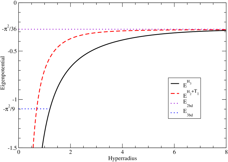
Figure 3: Eigenpotentials for $H_{3}$ and $H_{2}+T_{1}$

Using the index $j$ instead of $i$, but in the same manner, we note that the attractive part of the eigenpotential associated with $\overline{B}_{j_{0}}$ is simply weaker that of $B_{i_{0}}$, and will not sustain a 3-body bound state. The eigenpotential potential will however tend, for large values of $\rho$, to the same fixed negative energy, which is that of the 2-body bound state.

Finally for $T_{3}$ and for $(T_{2}+T_{1})$ , obviously there are only solutions for $E>0$.

Since they appear for the same set of equations as considered with interactions, but now without these interactions, we can associate them with the previous indices $i$ and $j$. The respective $B$’s and $\overline{B}$’s reduce to the corresponding hyperspherical harmonics.

Putting it all together …

For $E<0$, then, we see that we can subtract the contribution of the element stemming from $H_{3}$, from the corresponding element stemming from $(H_{2}+T_{1})$, and obtain the result

$$\frac{1}{\pi}\frac{d}{dq}[\delta^{i_{0}}(q)-\bar{\delta}^{j_{0}}(q)]$$ (33)

Essential is the fact that the coefficient of $\rho_{max}$ cancels !

For $E>0$, and $i$ and $j$ greater than $i_{0}$ and $j_{0}$, respectively, the terms deriving from $H_{3}$ and $T_{3}$ subtract, so as to eliminate the $\rho_{max}$ contribution, and so do the terms from $(H_{2}+T_{1})$ and $(T_{2}+T_{1})$.
We therefore obtain results such as:

$$\frac{1}{\pi}\frac{d}{dk}[\delta^{i}(k)-\bar{\delta}^{j}(k)],$$ (34)

where again again we can associate $i$ and $j$, and the $\rho_{max}$ contribution cancels.

For $i_{0}$ and $j_{0}$, the results from $H_{3}$ and $(H_{2}+T_{1})$ subtract, thereby eliminating the $\rho_{max}$ dependence. (See, below.)

In the adiabatic approximation, we can then write the following formula for the relative part of the complete trace, in the case of one 3-body bound-state + one 2-body bound state, associated with one eigenpotential:

$$Tr[(e^{-\beta H_{3}}-e^{-\beta T_{3}})-\,(e^{-\beta(H_{2}+T_{1})}-e^{-\beta(T_{2}+T_{1})})]=$$

$$\,e^{-\beta E_{3}}+\frac{1}{\pi}\int_{0}^{\infty}\!\!dk\!\,\frac{d}{dk}[\sum_{i>i_{0}}\delta^{i}(k)-\sum_{j>j_{0}}\bar{\delta}^{j}(k)]\,e^{-\beta(\frac{\hbar^{2}}{2m}k^{2})}$$

$$\hskip 71.13188pt+\,\frac{1}{\pi}\>e^{\beta\,\epsilon_{i_{0}}}\int_{0}^{\infty}\!\!dq\!\,\frac{d}{dq}[\delta^{i_{0}}(q)-\bar{\delta}^{j_{0}}(q)]\,e^{-\beta(\frac{\hbar^{2}}{2m}q^{2})}.$$ (35)

Alternatively, the last integral could be split into two, one from $0$ to $\overline{q}_{i_{0}}$, integrating over $q$, together with one from $\overline{q}_{i_{0}}$ to $\infty$, integrating over $k$. That is:

$$Tr[(e^{-\beta H_{3}}-e^{-\beta T_{3}})-\,(e^{-\beta(H_{2}+T_{1})}-e^{-\beta(T_{2}+T_{1})})]=$$

$$\,e^{-\beta E_{3}}+\frac{1}{\pi}\int_{0}^{\infty}\!\!dk\!\,\frac{d}{dk}[\sum_{all\,i}\delta^{i}(k)-\sum_{all\,j}\bar{\delta}^{j}(k)]\,e^{-\beta(\frac{\hbar^{2}}{2m}k^{2})}$$

$$\hskip 71.13188pt+\,\frac{1}{\pi}\>e^{\beta\,\epsilon_{i_{0}}}\int_{0}^{\overline{q}_{i_{0}}}\!\!dq\!\,\frac{d}{dq}[\delta^{i_{0}}(q)-\bar{\delta}^{j_{0}}(q)]\,e^{-\beta(\frac{\hbar^{2}}{2m}q^{2})}.$$ (36)

For simplicity, at this stage, we do not present formulas for the cases involving more bound states and eigenpotentials. They would be similar to the ones that we have just presented but involve more indices. [In the next section, we will consider a case with 4 eigenpotentials, with the same asymptotic behaviour, the same eigen-energy, and therefore the same $\epsilon_{i_{0}}$. We will sum the contributions of the 4 states.]

In another remark we note that in order for the $\rho_{max}$ contributions for $E<0$ to cancel, we need a one-to-one correspondence between the ‘bound-state’ eigenpotentials for $H_{3}$ and those for $H_{2}+T_{1}$. This will also be important in the results for $E>0$, when these eigenpotentials are involved.

McGuire’s Model With Attractive Forces

To show concrete details, and since to our knowledge there are no published results for this important case, we revisit our previous work with McGuire’s model of three particles in one dimension[11], but this time letting the delta function interactions be attractive. This would also be a prime example of the usefulness of adiabatic approximations.

A salient aspect of this model, with identical masses and interactions, is that there is no ”breakup”, i.e. there is no possibility of a system, characterized asymptotically by two bound particles and a free one, to evolve to a system characterized asymptotically by three free particles. To quote McGuire[12]: ”there are no new velocities generated even though there are three particles present”.

Similarly, when one considers the case of one particle that does not interact with the other two, which do interact but are of equal masses, there is no possibility of generating new velocities.

Technically, this manifests itself in that the R-matrix, associated with the S-matrix that characterizes the scattering of the 3 bodies, has off diagonal elements which are zero, when linking solutions of the two types of physical outcome mentioned above[18]. In our adiabatic-basis formalism our matrix $W$, related to the R-matrix by $R=-W^{-1}$, behaves similarly in the relevant off-diagonal elements. In our present work, we force the issue by using adiabatic approximations, thus insuring that solutions which have asymptotic forms associated with eigenpotentials that tend to zero for large $\rho$, and have non-zero amplitudes only for $E>0$, do NOT couple with the solutions associated with eigenpotentials that tend to a negative fixed-energy when $\rho$ becomes large.

We find then, thanks to this dichotomy, that the better part of our calculation is already done! The part, associated with the $\Lambda$’s that go to zero for large $\rho$, has already been calculated to first order in our previous article where no bound states appear; we need only an overall change in sign.

The expansions for the $q_{K}$’s that started with $(K+3)$ or $(K+1)$ now start with $(K-3)$ or $(K-1)$. The expressions for the $C$’s or the $D$’s now involve $(K-3)$ or $(K-1)$. The sums that used to start with $K=0$, $K=3$ for $H_{3}$ and $K=0$, $K=1$ for $H_{2}+T_{1}$ now, in the attractive case, start with $K=6$, $K=9$ for $H_{3}$ and $K=2$, $K=3$ for $H_{2}+T_{1}$.

Thus, to first order in $k$, the wave number, the sums and differences of the phase shifts (and their derivatives) remain identical to the results that we have previously achieved, apart from an overall change in sign. The contribution to the fugacity coefficient - which is additive to the other contributions that we must still calculate - also just changes in its sign.

Our result SO FAR is then:

$$b_{3}-b_{3}^{0}=+\frac{3\sqrt{2}}{4\pi g}\,\frac{1}{\beta}$$ (37)

where $\beta$ is the same variable that appears in Eq.(1), associated with the inverse of the temperature, and $g$ is the ‘strength’ of the delta functions in our model.

[We note that a factor of $(-1)^{m}$ is missing from Eqs.(13) and (15) of our previous article. The sine versions of our adiabatic bases should read:
For $H_{3}$ and $K=\textrm{odd},\,\,\,A_{K}(\rho)\,\,(-1)^{m}\,\sin(q_{K}(\vartheta-\frac{m\pi}{3}))$
For $H_{2}+T_{1}$ and $K=\textrm{odd},\,\,\,A^{12,3}_{K}(\rho)\,\,(-1)^{m}\,\sin(q_{K}(\vartheta-m\pi))$ ]

The new derivative terms

We mentioned that in the repulsive case the sums used to start with $K=0$, $K=3$ for $H_{3}$ and $K=0$, $K=1$ for $H_{2}+T_{1}$. In the attractive case, each of these cases is associated with a different eigenpotential, which however tends to a common plateau of energy $-\pi^{2}/36$, reflecting the asymptotic behaviour of the products: two bound particles (each time with the same binding energy) and a free one.

Below, we illustrate the behaviour of the eigenpotentials, adding the diagonal part of the adiabatic coupling elements, see Figure 4. We also show the linear behaviour of the phase shifts (calculated numerically) for small values of the $q_{K}$’s. See Figure 5.

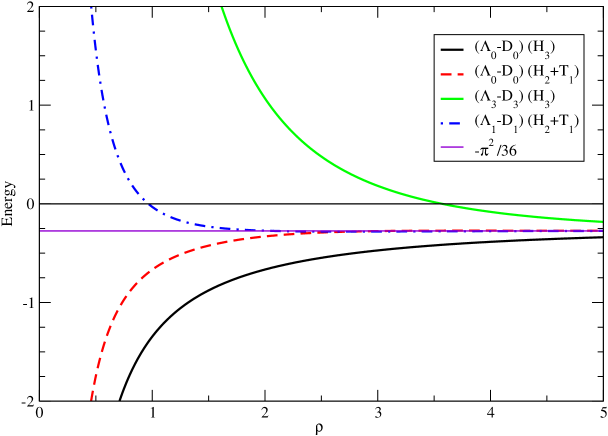
Figure 4: The diagonal part of the interactions for the four cases.

We note that to be consistent in our work, we only need the slope of the phases near the origin. For the case of $H_{3}$ and $K=0$, we will use the slope of the exact phase shift, as it is known and is associated with a zero energy resonance. See Appendix D.

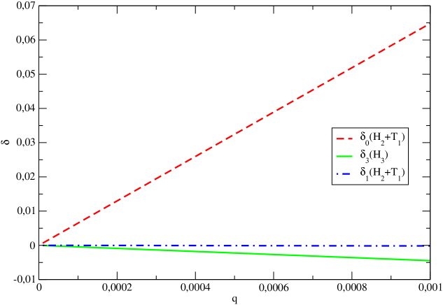
Figure 5: The low q behaviour of the phase shifts.

Taking the slopes of the phase shifts - and trying to round and keep significant digits - we find:
for $H_{3}$: $-8\sqrt{3}/\pi$, $-4.47$ for $K=0$ and $K=3$ respectively, and
for $H_{2}+T_{1}$: $64.91$ and $-.176$ for $K=0$ and $K=1$,
we obtain for the derivative of the sum of the $\delta$’s minus the sum of the $\overline{\delta}$’s: $-73.62$, of course rounding and trying to keep meaningful numerical results.

The bound state contribution in Eq.(35) now reads:

$$e^{\beta\frac{\hbar^{2}}{2m}\frac{\pi^{2}}{9}}+\frac{1}{\pi}\!e^{\beta\,\frac{\hbar^{2}}{2m}\,\frac{\pi^{2}}{36}}\,\,\frac{\sqrt{\pi}}{2}(-73.62)\sqrt{\frac{2m}{\beta\hbar^{2}}}$$ (38)

[To obtain the extra contribution to the fugacity coefficient, we need to multiply our result (above) by $\frac{\sqrt{3}}{\lambda_{T}}$. We also need to look at the contributions of ‘new’ oscillatory terms.]

The new oscillatory terms

Our work, here, parallels that which led to expression (34) in our previous paper.
For each of our four cases, $K=0,0,1,3\>$ we have to consider

$$\frac{1}{q}\,\sin(2q\rho_{max}+2\delta^{K})\;\;{\rm and}\;\;\frac{1}{k}\,\sin(2k\rho_{max}-K\pi+\pi/2)$$ (39)

where the first term is associated with an interaction which, in each case, asymptotically does not have any $1/\rho^{2}$ dependence, and must be integrated over $q$. The second term is a ‘no-interaction’ term, and must be integrated over $k$..

Let us consider the free or ’no-interaction’ terms in (39) namely

$$\frac{1}{k}\sin\left(2k\rho_{max}-K\pi+\frac{\pi}{2}\right)\ ,$$ (40)

$K=0,0,1,3$. In the past (no bound states) we have subtracted them directly from the interaction terms.. Here we cannot do so. However, since the number of terms considered in (39) is finite, the terms involved in the sum can be reordered and yield:

$$-\frac{1}{k}\sin\left(2k\rho_{max}+\frac{\pi}{2}\right)+\frac{1}{k}\sin\left(2k\rho_{max}+\frac{\pi}{2}\right)$$

$$-\frac{1}{k}\sin\left(2k\rho_{max}-3\pi+\frac{\pi}{2}\right)+\frac{1}{k}\sin\left(2k\rho_{max}-\pi+\frac{\pi}{2}\right)=0$$

We now consider the interaction terms (39), namely

$$\frac{1}{q}\sin\left(2q\rho_{max}+2\delta^{K}\right)\;{\rm and}\;\,\frac{1}{q}\sin\left(2q\rho_{max}+2{\bar{\delta}}^{K}\right)$$ (41)

for K=0,3 and K=0,1 respectively.
We recall that we call $\delta$’s the phases for $H_{3}$, and ${\bar{\delta}}$’s for $H_{2}+T_{1}$.

These phases go to zero as $q\rightarrow 0$, except for the symmetric case $K=0$, where $\delta=3\pi/2$. This is important because in the resulting integrals, upon the change of variables to $y$, see below, each $\delta$ will be evaluated as $\delta(y/{2q\rho_{max}})$, in the limit of $\rho_{max}\rightarrow\infty$. This implies that the expression

$$\frac{1}{q}\sin(2q\rho_{max}+2\delta^{0})-\frac{1}{q}\sin(2q\rho_{max}+2{\bar{\delta}}^{0})$$

$$+ \frac{1}{q}\sin(2q\rho_{max}+2\delta^{3})-\frac{1}{q}\sin(2q\rho_{max}+2{\bar{\delta}}^{1})$$

is equal to

$$-2\frac{1}{q}\sin\left(2q\rho_{max}\right)\ .$$ (42)

The contribution of the oscillatory term to the final integral then reads

$$\frac{\sqrt{3}}{\lambda_{T}}\int_{0}^{\infty}dq\frac{1}{2\pi}\left[-2\frac{1}{q}\sin(2q\rho_{max})\right]\exp\left(-\beta\frac{\hbar^{2}}{2m}\left[q^{2}-\frac{\pi^{2}}{36}\right]\right)$$ (43)

Setting $y=2q\rho_{max}$ we have

$$I=-\frac{\sqrt{3}}{\lambda_{T}}(\frac{1}{\pi})\,\int_{0}^{\infty}dy\frac{\sin y}{y}\exp\left(-\beta\frac{\hbar^{2}}{2m}\left[\left(\frac{y}{2\rho_{max}}\right)^{2}-\frac{\pi^{2}}{36}\right]\right)$$ (44)

which, at the limit $\rho_{max}$ infinite, yields

$$I=-\frac{\sqrt{3}}{2\lambda_{T}}\,e^{\beta(\hbar^{2}/2m)(\pi^{2}/36)}$$ (45)

Our result

Recalling that:

$$c=(2m/\hbar^{2})(3g/\pi\sqrt{2}),\ \ g=(\hbar^{2}/2m)(\pi\sqrt{2}c/3),\ \ \lambda_{T}=(2\pi\hbar^{2}\beta/m)^{1/2},$$ (46)

and that the following result is for the particular value of $c=-1$, we obtain:

$$b_{3}-b_{3}^{0}=\frac{\sqrt{3}}{\lambda_{T}}\left(e^{\lambda_{T}^{2}(\pi/36)}-\frac{1}{2}\,e^{\lambda_{T}^{2}(\pi/144)}\right)+\frac{1}{\lambda_{T}^{2}}\left(-\frac{9}{\pi}+\sqrt{3}\,(-73.62)\,e^{\lambda_{T}^{2}(\pi/144)}\right)\,.$$ (47)

We note that the energies in the exponentials correspond to the energy of the three-body bound state: $-(\hbar^{2}/2m)(\pi^{2}/9)\,c^{2}$, and that of the two-body bound state:
$-(\hbar^{2}/2m)(\pi^{2}/36)\,c^{2}$. The numerical value $(-73.62)$ is, of course, a result that has been rounded.

The Full Generalization

Assume now that for $H_{3}$ we have one 3-body bound state and (asymptotically) two possibilities of a 2-body bound state, each corresponding to one eigenpotential, and introduce amplitudes. This will be the simplest example that reveals the details that we must deal with in general. The asymptotic behaviour will be as follows.
The upper index $i$ will identify the overall solution, corresponding to $\psi^{i}$ in Eq.(26). The $\ell$’s will denote the amplitudes. For us, in our example, $\ell_{0}$ is associated with the adiabatic eigenfunction $B_{\ell_{0}}$, the lowest eigenpotential, and $B_{\ell_{1}}$ with the second lowest. Letting also, to simplify the notation, $q=q_{0}=q_{\ell_{0}}$ !

For $E>0$ and $\ell>\ell_{0},\ell_{1}$, and for the values $\ell_{0},\ell_{1}$ we have then:

$$\!\!\!\!\!\!\!\!\!\phi^{i}_{\ell}(q,\rho)\rightarrow(q\rho)^{1/2}{\cal C}_{\ell}^{i}(q)\,[\cos\delta^{i}(q)\,J_{K_{\ell}+2}(k\rho)-\sin\delta^{i}(q)\,N_{K_{\ell}+2}(k\rho)]$$ (48)

$$\;\phi^{i}_{\ell_{1}}(q,\rho)\rightarrow(q\rho)^{1/2}{\cal C}_{\ell_{1}}^{i}(q)\,[\cos\delta^{i}(q)\,J_{K_{\ell_{1}}+2}(q_{\ell_{1}}\rho)-\sin\delta^{i}(q)\,N_{K_{\ell_{1}}+2}(q_{\ell_{1}}\rho)]$$ (49)

$$\;\phi^{i}_{\ell_{0}}(q,\rho)\rightarrow(q\rho)^{1/2}{\cal C}_{\ell_{0}}^{i}(q)\,[\cos\delta^{i}(q)\,J_{K_{\ell_{0}}+2}(q\rho)-\sin\delta^{i}(q)\,N_{K_{\ell_{0}}+2}(q\rho)]$$ (50)

If we then use our procedure as before, summing over the contributions of all of the amplitudes corresponding to the solution $i$, we obtain for the integral over $\rho$:

$$\frac{1}{\pi}\frac{d}{dq}\delta^{i}(q)+\frac{\rho_{max}}{\pi}\left(\sum_{\ell\neq\ell_{0},\ell_{1}}|{\cal C}_{\ell}^{i}(q)|^{2}\frac{q}{k}+|{\cal C}_{\ell_{1}}^{i}(q)|^{2}\frac{q}{q_{\ell_{1}}}+|{\cal C}_{\ell_{0}}^{i}(q)|^{2}\right)$$ (51)

To obtain the first term, we have use the fact that $\cal C$ is an orthogonal matrix, and that therefore $\sum_{\ell}|{\cal C}^{i}_{\ell}|^{2}=1$ .

For $E<0$, we have to consider two possibilities: $0<E<-\epsilon_{\ell_{1}}$ and $-\epsilon_{\ell_{1}}<E<-\epsilon_{\ell_{0}}$, where $-\epsilon_{\ell_{1}}$ and $-\epsilon_{\ell_{0}}$ are the respective energies of the two 2-body bound states, the ${\ell_{0}}$ bound state being the deepest. We will then have:

For $0<E<-\epsilon_{\ell_{1}}$,

$$\phi^{i}_{\ell_{1}}(q,\rho)\rightarrow(q\rho)^{1/2}{\cal C}^{i}_{\ell_{1}}(q)[\cos\delta^{i}(q)\,J_{K_{\ell_{1}}+2}(q_{\ell_{1}}\rho)-\sin\delta^{i}(q)\,N_{K_{\ell_{1}}+2}(q_{\ell_{1}}\rho)]$$ (52)

$$\phi^{i}_{\ell_{0}}(q,\rho)\rightarrow(q\rho)^{1/2}{\cal C}^{i}_{\ell_{0}}(q)[\cos\delta^{i}(q)\,J_{K_{\ell_{0}}+2}(q\rho)-\sin\delta^{i}(q)\,N_{K_{\ell_{0}}+2}(q\rho)]$$ (53)

which then yields

$$\frac{1}{\pi}\frac{d}{dq}\delta^{i}(q)+\frac{\rho_{max}}{\pi}\left(|{\cal C}_{\ell_{1}}^{i}(q)|^{2}\frac{q}{q_{\ell_{1}}}+|{\cal C}_{\ell_{0}}^{i}(q)|^{2}\right)$$ (54)

Finally, for $-\epsilon_{\ell_{1}}<E<-\epsilon_{\ell_{0}}$, we will have

$$\phi^{i}_{\ell_{0}}(q,\rho)\rightarrow(q\rho)^{1/2}[\cos\delta^{i}(q)\,J_{K_{\ell_{0}}+2}(q\rho)-\sin\delta^{i}(q)\,N_{K_{\ell_{0}}+2}(q\rho)]$$ (55)

which gives

$$\frac{1}{\pi}\frac{d}{dq}\delta^{i}(q)+\frac{\rho_{max}}{\pi}$$ (56)

For $(H_{2}+T_{1})$, the discussions and the expressions follow in a similar fashion.
We will change $i$ to $j$, $\ell$ to $r$. We will let $q=q_{0}=q_{{\ell}_{0}}=q_{r_{0}}$.
It is clear, since the reference is to the energy associated with the 2-body bound state, that the deepest (lowest) energy of the $H_{2}+T_{1}$ system will be same as for the $H_{3}$ system. The range of the wave number integration in the two cases, will be the same. For the equivalent of Eq.(51), we will have:

$$\frac{1}{\pi}\frac{d}{dq}\bar{\delta}^{j}(q)+\frac{\rho_{max}}{\pi}\left(\sum_{r\neq{r_{0}},{r}_{1}}|{\cal(C^{\prime})}_{r}^{j}(q)|^{2}\frac{q}{k}+|{\cal(C^{\prime})}_{r_{1}}^{j}(q)|^{2}\frac{q}{q_{r_{1}}}+|{\cal(C^{\prime})}_{r_{0}}^{j}(q)|^{2}\right)$$ (57)

where $q_{r_{1}}$ will be equal $q_{\ell_{1}}$, the energy of the second 2-body bound state being equal in the two cases!

If we look to subtract the $\rho_{max}$ terms for $H_{3}$ from those of $H_{2}+T_{1}$, we note the following. First, while in our McGuire example there were as many eigenpotentials associated with $H_{3}$ as with $H_{2}+T_{1}$, we don’t see that this would necessarily apply in the general case. Second, even if this were to be the case, if we compare the $\cal{C}$’s and their factors in the two situations, we see no reason why the $\rho_{max}$ terms should cancel. Of course, they would do so in the adiabatic case.

The situation is now clear.

We have a simple formula that we can use in general, which involves the energies of the appropriate 3-body bound states and integrals over sums of the derivative of respective phase shifts, in addition to $\rho_{max}$ terms. We shall need to discuss the latter in the next section.

The volume independent result for the 3-body fugacity cluster, is then given by:

$$b_{3}-b_{0}=\frac{3^{3/2}}{\lambda^{3}_{T}}\left(\sum_{m}e^{-\beta E_{3,m}}+\frac{1}{\pi}\int_{0}^{\infty}\!\!dq\!\,\left[\sum_{all\,i}\frac{d}{dq}\delta^{i}(q)-\sum_{all\,j}\frac{d}{dq}\bar{\delta}^{j}(q)\right]\,e^{-\beta(\frac{\hbar^{2}}{2m}q^{2}-\epsilon_{2,0})}\right)$$ (58)

A comment about oscillatory terms. They will not contribute unless, as $q\rightarrow 0$, the phases are not zero or an integral multiple of $\pi$. In three dimensions, this will not occur unless there is a zero-energy resonance or a half-bound state. In one dimension, this may occur even in the two-body problem and a repulsive force[16], where we have found that $\delta(0)=-\pi/2$, for a delta function interaction.

Perspective

Our phase shift formula makes sense to us.

In previous work, under the constraints of positive potentials and Boltzmann statistics, we were able to show that, in a semi-classical approximation, the phase shift sums in our quantum mechanical formulation lead to the correct classical expressions for the 3-body cluster. Each sum was shown to be associated with a classical expression for an integrand, involving the potential terms, which integrated over the position variables, diverges as the volume increases to infinity. When all of the terms of the cluster are taken together, the resulting integral is finite and volume independent.

Terms in $\rho_{max}$ play no role in this, and in our previous work using McGuire’s model with repulsive potentials, as well as in the present work with attractive forces, we see that the $\rho_{max}$ terms cancel out. Unfortunately we cannot demonstrate this in general. Since these terms are not tied to potentials, we feel that they are artifacts, of no fundamental importance.

Another aspect is of interest.

In an important paper, Mazo[19] noted that using the asymptotic expression [here, argument much larger than the order] for the wave functions used to calculate the partition function of one particle in a box (a sphere), leads to an incorrect result. ‘The important angular momenta $\ell$ are very large and increase proportionately with the size of the sphere.’ An improved calculation yields the correct result.

Mazo determined, however, that the phase shift formula for the 2-body cluster (virial) problem was correct, because the sum involved only a few angular momenta. The issue merits further discussion.

Both in the 2-body expressions and in ours, there is an integration over the energy (or the wave number). The effective range of the energy is limited by a Boltzmann factor, such that, for a given temperature and accuracy, there is an upper limit to the energy to be considered.

For the 2-body system, for a finite range of the interaction, say ‘a’, there is then a semi-classical argument, which can be extended appropriately in the full quantum mechanics, which indicates that the ‘higher’ angular momenta $\ell>k_{max}a$ are not involved in the scattering (or in the full quantum mechanics, for sufficiently large $\ell$, only in an exponentially decreasing fashion).

Now, in our case, and that is the intuitive argument presented in our first paper[3], we presented an analogous argument for the 3-body cluster, which also has - in position space - a finite extent (which is why it was devised). I.e., the cluster has been constructed so that it only contributes when particles are involved in a truly three-body event.

In the 3-body problem, when describing the collision, the Global Angular Momentum ($K$ being the order) measures how closely three bodies simultaneously approach each other[20]. A semi-classical point of view would then suggest that only a limited (or convergent) number of the higher K angular functions would be required to correctly describe the properties of the cluster, at a given energy.

Of course, our adiabatic basis is quite superior to the original hyperspherical basis used in our first paper, but asymptotically, for 3-3 scattering, it reduces to hyperspherical harmonics. We think that the argument that we have presented is a dependable guide.

In our work with McGuire’s model, we had the advantage of being able to obtain analytical results. In our previous paper - and in this one, in which we also use the same result - we evaluate the difference of two sums, each over an infinite number of phase shifts, but for which the difference converges. To obtain this difference, we had to use a procedure due to Abel to help with the summations.

For the third cluster in 2-dimension[5, 7], analytical and numerical data considerations led to the vanishing of the leading part of the first Born contribution to the authors’ equivalent to our $G(k)$, Eq.(24). This led to the correct threshold behaviour of the $G(k)$ and the definite demonstration of convergence for small values of $k$.

As we can see, there are sensitive issues and a combination of analytical and numerical results is really required, if one is to take advantage of the formalism that we have proposed and now extended.

Finally, we have always emphasized that our hyperspherical-adiabatic method could be extended to more particles (and dimensions). Higher clusters, however, would mean more phase shift sums and more subtractions!

Conclusions

The effort that led to this paper, is the last in a long sequence of efforts, starting with an early formulation of the third cluster (or virial) in terms of hyperspherical harmonics, all in an attempt to generalize the formula of Ulhenbeck and Beth, and of Gropper, to the higher clusters and virials.

It led to formulations in the continuum, out of the box; to the consideration of the second virial with anisotropic interactions ; to the usefulness of an adiabatic approximation in using our hyperspherical formalism, and then reformulations in terms of an adiabatic basis. It led, importantly, within constraints, to devising a WKB + adiabatic approximation, a semi-classical approach, so as to obtain the classical expressions from the eigenphase shift formalism, as it existed then.

It led to work in two dimensions and to our obtaining (together with our Russian friends) a wealth of analytical results (adiabatic basis, eigenpotentials, eigenphase shifts, W-matrix, S-matrix), for one-dimensional delta function models.

Finally, now, in the present paper, we present our most elegant, our most general result, our full generalization of the famous Ulhenbeck and Beth formula. We have gone as far as we could. In the previous section, Perspective, we have tried to draw attention to sensitive aspects, and perhaps limitations, of the phase shift approach.

To complement the work, we have calculated explicitly, in an adiabatic approximation, the $b_{3}$ cluster for the attractive version of McGuire’s model. To our knowledge, this is also new.

Acknowlegments

Alejandro Amaya thanks the partial support, in the early stages of this work, of the DGAPA, program PAPIIT-IN109511, and Sigurd Larsen thanks the always welcoming hospitality of the Institutes, the ICF of Mexico and the IPN Orsay.

In this, the last of the long sequence of papers that have lead to our results, SYL wishes to thank his many collaborators over the years, and especially his present coauthors, who in friendship and intellectual support and contribution have been essential to the communal effort. These papers would not have been possible without their help and contributions. The value of their friendship has been inestimable.

Appendix A

The eigenphase-shift eigenfunctions

In this Appendix we show, in a more detailed fashion than shown in ([8]), that we can choose solutions, for finite sets of coupled equations from Eq. (11), such that a unique eigenphase shift characterizes the asymptotic behaviour of each of these solutions. We simplify the discussion, in a manner appropriate to our section ‘Without Bound States’. We append a ‘coda’ to generalize our discussion to include bound states, and possible excited states in the asymptotic states. The point is then, that for the following discussion, the eigenpotentials go to zero, as $\rho$ approaches infinity.

Without Bound States and Excited States

Changing notation, so as to ultimately connect with asymptotic solutions $i$ of Eq. (11) for $\rho$ large, with components labeled by the index $\ell$, we note that ALL the solutions of (11) can, for finite sets (however large), and for sufficiently large values of $\rho$, be written in the form

$${\chi}_{\ell}^{\lambda}\left(k,\rho\right)\rightarrow\left(k\rho\right)^{1/2}\left[A^{\lambda}_{\ell}\left(k\right)\,J_{K_{\ell}+2}\left(k\rho\right)+B^{\lambda}_{\ell}\left(k\right)\,N_{K_{\ell}+2}\left(k\rho\right)\right],$$ (59)

where $K_{\ell}$ is one of the quantum labels included in the index $\ell$, and $\lambda$ denotes the solution. The linear combinations,

$$\begin{array}[]{cl}\zeta_{\ell}^{\mu}\left(k,\rho\right)&={\displaystyle{\displaystyle{\displaystyle{\displaystyle\sum_{\lambda}}}}\chi_{\ell}^{\lambda}\left(k,\rho\right)\left[A^{-1}\right]^{\mu}_{\lambda}\left(k\right)}\\ \vspace{.1cm}\hfil&\sim\left(k\rho\right)^{1/2}\left[\delta^{\mu}_{\ell}\,J_{K_{\ell}+2}\left(k\rho\right)+W_{\ell}^{\mu}\left(k\right)\,N_{K_{\ell}+2}\left(k\rho\right)\right],\end{array}$$ (60)

are of particular interest, because the matrix $W$, with elements defined by

$$W_{\ell}^{\mu}\left(k\right)={\displaystyle{\displaystyle{\displaystyle\sum_{\lambda}}B^{\lambda}_{\ell}\left(k\right)}}\left[A^{-1}\right]^{\mu}_{\lambda}\left(k\right),$$ (61)

is symmetric (as it is shown in Appendix B). In our case, the $W$ matrix is also real, so it can be diagonalized by a real orthogonal matrix ${\mathcal{C}}$, leading to a unique eigenphase shift, for each solution, associated with all components of each of the new solutions. This important property is demonstrated by multiplying the functions defined in Eq. (60) by the matrix elements of ${\mathcal{C}}$. Then by using the definition of the orthogonal matrix

$${\displaystyle\sum_{i^{\prime}}}{\mathcal{C}}^{i^{\prime}}_{\ell}\left(k\right)\left[{\mathcal{C^{T}}}\right]^{\mu^{\prime}}_{i^{\prime}}\left(k\right)=\delta^{\mu^{\prime}}_{\ell}$$

and defining the eigenphase shift in terms of the $W$ eigenvalues as

$${\displaystyle\sum_{\mu^{\prime}}}\left[{\mathcal{C}}^{T}\right]^{\mu^{\prime}}_{i^{\prime}}\left(k\right)\left[\sum_{\mu}{\displaystyle W_{\mu^{\prime}}^{\mu}\left(k\right)}\,{\mathcal{C}}^{i}_{\mu}\left(k\right)\right]=-\delta_{i^{\prime}}^{i}\,\tan\left(\delta^{i}(k)\right),$$

we obtain the desired solution, with a unique eigenphase shift shared by each of its components,

$$\begin{array}[]{cl}\tilde{\phi}_{\ell}^{i}\left(k,\rho\right)&={\displaystyle\sum_{\mu}}{\displaystyle\zeta_{\ell}^{\mu}\left(k,\rho\right)}\,\,{\mathcal{C}}^{i}_{\mu}\left(k\right)\\ \\ &\sim\left(k\rho\right)^{1/2}{\mathcal{C}}^{i}_{\ell}\left(k\right)\,\left[J_{K_{\ell}+2}\left(k\rho\right)-\tan\left(\delta^{i}(k)\right)\,N_{K_{\ell}+2}\left(k\rho\right)\right].\end{array}$$

With Bound States, or/and Excited States

Essentially, we have the same type of asymptotic formulae:

$$\begin{array}[]{cl}\tilde{\phi}_{\ell}^{i}\left(q_{\alpha},\rho\right)&={\displaystyle\sum_{\mu}}{\displaystyle\zeta_{\ell}^{\mu}\left(q_{\alpha},\rho\right)}\,\,{\mathcal{C}}^{i}_{\mu}\left(q_{\alpha}\right)\\ \\ &\sim\left(q_{\alpha}\rho\right)^{1/2}{\mathcal{C}}^{i}_{\ell}\left(q_{\alpha}\right)\,\left[J_{K_{\ell}+2}\left(q_{\beta}\rho\right)-\tan\left(\delta^{i}(q_{\alpha})\right)\,N_{K_{\ell}+2}\left(q_{\beta}\rho\right)\right].\end{array}$$

but the $q_{\beta}$ depends on the kinetic energy, which, asymptotically, we find in the fragment channels, and the $q_{\alpha}$ which depends on what the integration variable is over the energy, such that each amplitude has a delta function normalization. We refer to our ref([8]).

Appendix B

In this appendix we show that the matrix $W$ (61) is symmetric, using the same approach followed in reference [8].

Without Bound States and Excited States

Let us consider a solution $\zeta^{\mu}$ of Eq. (11) (see Eq. (60)). Then from the relation

$${\displaystyle\sum_{\ell}}\left[\zeta_{\ell}^{\mu}\left(k,\rho\right){\cal O}\left(k^{\prime},\rho\right)\zeta_{\ell}^{\mu^{\prime}}\left(k^{\prime},\rho\right)-\zeta_{\ell}^{\mu^{\prime}}\left(k^{\prime},\rho\right){\cal O}\left(k,\rho\right)\zeta_{\ell}^{\mu}\left(k,\rho\right)\right]=0,$$ (62)

where

$$\begin{array}[]{cl}{\cal O}\left(k,\rho\right)\zeta_{\ell}^{\mu}\left(k,\rho\right)&=\left(\frac{d^{2}}{d\rho^{2}}-\Lambda_{\ell}\left(\rho\right)+k^{2}\right)\zeta_{\ell}^{\mu}\left(k,\rho\right)\\ &+2{\displaystyle\sum_{\ell^{\prime}}}C_{\ell}^{\ell^{\prime}}\left(\rho\right)\frac{d}{d\rho}\zeta_{\ell^{\prime}}^{\mu}\left(k,\rho\right)\\ &+{\displaystyle\sum_{\ell^{\prime}}}D_{\ell}^{\ell^{\prime}}\left(\rho\right)\zeta_{\ell^{\prime}}^{\mu}\left(k,\rho\right),\end{array}$$ (63)

we obtain the identity

$$\begin{array}[]{l}{\displaystyle\sum}\frac{d}{d\rho}\left[\zeta_{\ell}^{\mu}\left(k,\rho\right)\frac{d}{d\rho}\zeta_{\ell}^{\mu^{\prime}}\left(k^{\prime},\rho\right)-\zeta_{\ell}^{\mu^{\prime}}\left(k^{\prime},\rho\right)\frac{d}{d\rho}\zeta_{\ell}^{\mu}\left(k,\rho\right)\right]\\ \ell\\ =\left\{\left(k^{\prime}{}^{2}-k^{2}\right){\displaystyle\sum_{\ell}}\zeta_{\ell}^{\mu^{\prime}}\left(k^{\prime},\rho\right)\zeta_{\ell}^{\mu}\left(k,\rho\right)\right.\\ \\ \left.+2{\displaystyle\sum_{\ell,\ell^{\prime}}}\frac{d}{d\rho}\left[\zeta_{\ell}^{\mu}\left(k,\rho\right)\,C_{\ell}^{\ell^{\prime}}\left(\rho\right)\,\zeta_{\ell^{\prime}}^{\mu^{\prime}}\left(k^{\prime},\rho\right)\right]\right\}.\end{array}$$ (64)

where, for the last term, we used Eq.(13). Integrating over $\rho$ when $k=k^{\prime}$ leads us to the following equation,

$$\begin{array}[]{l}{\displaystyle\sum_{\ell}}\left[\zeta_{\ell}^{\mu}\left(k,\rho\right)\frac{d}{d\rho}\zeta_{\ell}^{\mu^{\prime}}\left(k,\rho\right)-\zeta_{\ell}^{\mu^{\prime}}\left(k,\rho\right)\frac{d}{d\rho}\zeta_{\ell}^{\mu}\left(k,\rho\right)\right]_{\rho=\rho_{max}}=0.\end{array}$$ (65)

We used the fact that $\zeta_{\ell}^{\mu}$ goes to zero as $\rho$ itself goes to zero, and that $C_{\ell}^{\ell^{\prime}}$ decreases fast enough for $\rho$ large. We can then substitute, in the above expression, the asymptotic form of the solutions, Eq. (60) in appendix A, valid for large $\rho$. We obtain

$$\begin{array}[]{cl}0=&k\rho\left(W_{\mu}^{\mu^{\prime}}\left(k\right)-W_{\mu^{\prime}}^{\mu}\left(k\right)\right)\,\left(J_{K_{\ell}+2}\left(k\rho\right)\,\frac{d}{d\rho}\left[\left(k\rho\right)^{1/2}N_{K_{\ell}+2}\left(k\rho\right)\right]\right.\\ \\ &\left.-N_{K_{\ell}+2}\left(k\rho\right)\frac{d}{d\rho}\left[\left(k\rho\right)^{1/2}J_{K_{\ell}+2}\left(k\rho\right)\right]\right)\end{array}$$ (66)

The evaluation of the Wronskian for the Bessel’s functions [21], leads to the equality

$$W_{\mu}^{\mu^{\prime}}\left(k\right)=W_{\mu^{\prime}}^{\mu}\left(k\right),$$ (67)

which proves that the matrix $W$ is symmetric.

With Bound States, or/and Excited States

The appropriate asymptotic formulae would change the Eq.(66) into the following equation:

$$\begin{array}[]{cl}0=&q_{\alpha}\rho\left(W_{\mu}^{\mu^{\prime}}\left(q_{\alpha}\right)-W_{\mu^{\prime}}^{\mu}\left(q_{\alpha}\right)\right)\,\left(J_{K_{\ell}+2}\left(q_{\beta}\rho\right)\,\frac{d}{d\rho}\left[\left(q_{\alpha}\rho\right)^{1/2}N_{K_{\ell}+2}\left(q_{\beta}\rho\right)\right]\right.\\ \\ &\left.-N_{K_{\ell}+2}\left(q_{\beta}\rho\right)\frac{d}{d\rho}\left[\left(q_{\alpha}\rho\right)^{1/2}J_{K_{\ell}+2}\left(q_{\beta}\rho\right)\right]\right)\end{array}$$ (68)

where $q_{\alpha}$ and $q_{\beta}$ have the same meaning as in Appendix A. From the above relation we can prove the same symmetric property, Eq. (67), for the matrix W.

Appendix C

In this Appendix we develop formulae associated to the four lowest eigensolutions of Eq.(9), corresponding to $K=0,3$ (Cosine basis) and $K=0,1$ (Sine basis), for the system of three particles on a line interacting through delta function potentials. A few of them appeared in our previous works. See [17], Eqs. (26,33,34) and also [22], Eqs. (A1).

Cosine basis

For $K=0$ the adiabatic function basis reads :

$$B_{0}(\rho,\theta)=\sqrt{N}\ \ \cos(q_{0}\theta),$$ (69)

where

$$\begin{array}[]{rllll}\theta\in[-\pi/6,\pi/6]&\mathrm{and}\qquad q_{0}\tan\left(q_{0}\frac{\pi}{6}\right)&=-\frac{\pi\rho}{6}&{\rm for}&{\rm H_{3}},\\ \\ \theta\in[-\pi/2,\pi/2]&\mathrm{and}\qquad q_{0}\tan\left(q_{0}\frac{\pi}{2}\right)&=-\frac{\pi\rho}{6}&{\rm for}&{\rm(H_{2}+T_{1})},\end{array}$$ (70)

and the normalization factors may be written as

$$\begin{array}[]{rlll}N&=\int_{-\pi/6}^{\pi/6}\cos^{2}(q_{0}\theta)\ {\rm d}\theta&=\frac{\pi}{6}\left(1-\frac{\rho}{q_{0}^{2}+\pi^{2}\rho^{2}/36}\right)&{\rm for\ H_{3}},\\ \\ N&=\int_{-\pi/2}^{\pi/2}\cos^{2}(q_{0}\theta)\ {\rm d}\theta&=\frac{\pi}{2}\left(1-\frac{\rho/3}{q_{0}^{2}+\pi^{2}\rho^{2}/36}\right)&{\rm for(\ H_{2}+T_{1})}\ .\end{array}$$ (71)

We observe that the equations in (70) imply that

$$(\forall\rho)\qquad\quad\ q_{0}^{(H_{2}+T_{1})}(\rho)=q_{0}^{(H_{3})}(3\rho)/3\ .$$ (72)

The introduction of the above relation in the definitions of $\Delta$ and $\Lambda$,

$$\Lambda_{0}(\rho)=\Delta_{0}-\frac{1/4}{\rho^{2}};\quad\Delta_{0}=\frac{q_{0}^{2}(\rho)}{\rho^{2}}$$ (73)

and in the definition of $D$ (see Eq. (12)) leads us to write the relations beetwen variables in the cases, $H_{3}\,\mathrm{and\,}(H_{2}+T_{1})$ as:

$$\begin{array}[]{rlll}(\forall\rho)&\qquad\quad\Delta_{0}^{(H_{2}+T_{1})}(\rho)&=&\Delta_{0}^{(H_{3})}(3\rho)\\ \\ (\forall\rho)&\qquad\quad\Lambda_{0}^{(H_{2}+T_{1})}(\rho)&=&\Lambda_{0}^{(H_{3})}(3\rho)-\frac{2}{\left(3\rho\right)^{2}}\\ \\ (\forall\rho)&\qquad\quad\ D_{0,0}^{(H_{2}+T_{1})}(\rho)&=&9D_{0,0}^{(H_{3})}(3\rho)\ .\end{array}$$ (74)

Next, for small $\rho$ we collect the expansions in powers of $\rho$ for $q_{0}$, $\Lambda_{0}$ and $D_{0,0}$ in the case of $H_{3}$:

$$q_{0}(\rho) = i\sqrt{\rho}\left(1+\frac{\pi^{2}}{216}\ \rho+\frac{11\pi^{4}}{466560}\ \rho^{2}+\frac{17\pi^{6}}{235146240}\ \rho^{3}-\frac{281\pi^{8}}{1015831756800}\ \rho^{4}\right.$$ (75)

$$\left.-\frac{44029\pi^{10}}{7240848762470400}\ \rho^{5}+\dots,\right)$$

$$\Lambda_{0}(\rho) = -\frac{1}{4\rho^{2}}-\frac{1}{\rho}-\frac{\pi^{2}}{108}-\frac{\pi^{4}}{14580}\ \rho-\frac{\pi^{6}}{2755620}\ \rho^{2}-\frac{\pi^{8}}{1488034800}\ \rho^{3}$$ (76)

$$+\frac{\pi^{10}}{88389267120}\ \rho^{4}+\ldots,$$

$$D_{0,0}(\rho) = -\frac{\pi^{4}}{58320}-\frac{\pi^{6}}{2204496}\ \rho-\frac{31\ \pi^{8}}{5952139200}\ \rho^{2}-\frac{\pi^{10}}{117852356160}\ \rho^{3}$$ (77)

$$\left.+\frac{1151\ \pi^{12}}{1608684661584000}\ \rho^{4}+\ldots\right)$$

The corresponding expansions for large $\rho$ would be:

$$q_{0}\left(\rho\right) = \frac{6i}{\pi}\ (\alpha+2\alpha\exp(-2\alpha)),\qquad\quad\alpha=\frac{\pi^{2}\rho}{36};$$

$$\Lambda_{0}\left(\rho\right) = -\frac{\pi^{2}}{36}-\frac{1}{4\ \rho^{2}}-\frac{\pi^{2}}{9}\exp(-\pi^{2}\rho/18)+\dots,$$ (78)

$$D_{0,0}\left(\rho\right) = -\frac{1}{4\ \rho^{2}}-\pi^{2}\left(\frac{\pi^{4}\ \rho}{17496}-\frac{\ \pi^{2}}{324}-\frac{1}{18\ \rho}\right)\exp(-\pi^{2}\rho/18)+\dots$$

and the analogous expressions for both, small $\rho$ and $\rho$ large, in the case of $(H_{2}+T_{1})$ can be obtained from Eqs. (72, 74 and 74 ).

Note that the diagonal part of the asymptotic adiabatic interactions, $\Lambda_{0}\left(\rho\right)-D_{0,0}\left(\rho\right)$, approaches exponentially the two-body bound energy $-\pi^{2}/36$. (See Fig. 4).

Sine basis

The adiabatic basis reads :

$$B_{K}(\rho,\theta)=\sqrt{N}\ \sin(q_{K}\theta)$$ (79)

where

$$\begin{array}[]{rllll}\theta\in[-\pi/6,\pi/6]&\mathrm{and}\ q_{3}\cot\left(q_{3}\frac{\pi}{6}\right)&=-\frac{\pi\rho}{6}&{\rm for}&{\rm H_{3}},\\ \\ \theta\in[-\pi/2,\pi/2]&\;\mathrm{and\;}q_{1}\cot\left(q_{1}\frac{\pi}{2}\right)&=-\frac{\pi\rho}{6},&{\rm for}&{\rm(H_{2}+T_{1})},\end{array}$$ (80)

and the normalization factors may be written as

$$\begin{array}[]{rlll}N&=\int_{-\pi/6}^{\pi/6}\cos^{2}(q_{3}\theta)\ {\rm d}\theta&=\frac{\pi}{6}\left(1-\frac{\rho}{q_{3}^{2}+\pi^{2}\rho^{2}/36}\right)&{\rm for\ H_{3}},\\ \\ N&=\int_{-\pi/2}^{\pi/2}\cos^{2}(q_{1}\theta)\ {\rm d}\theta&=\frac{\pi}{2}\left(1-\frac{\rho/3}{q_{1}^{2}+\pi^{2}\rho^{2}/36}\right)&{\rm for\ (H_{2}+T_{1})}\ .\end{array}$$ (81)

The equations in (80) imply that

$$(\forall\rho)\qquad\quad q_{1}^{(H_{2}+T_{1})}(\rho)=q_{3}^{(H_{3})}(3\rho)/3\ .$$ (82)

Hence, taking into account that

$$\Delta_{K}=\frac{q_{K}^{2}(\rho)-K^{2}}{\rho^{2}};\quad K>0,$$ (83)

$$\Lambda_{K}=\frac{q_{K}^{2}(\rho)-1/4}{\rho^{2}};\quad K>0,$$ (84)

and the definition of the matrix $D$ (Eq.(12)), we can write:

$$(\forall\rho)\ \qquad\quad\Delta_{1}^{(H_{2}+T_{1})}(\rho) = \Delta_{3}^{(H_{3})}(3\rho)\ ,$$ (85)

$$(\forall\rho)\ \qquad\quad\Lambda_{1}^{(H_{2}+T_{1})}(\rho) = \Lambda_{3}^{(H_{3})}(3\rho)-\frac{2}{\left(3\rho\right)^{2}}\ ,$$ (86)

$$(\forall\rho)\qquad\quad\ D_{1}^{(H_{2}+T_{1})}(\rho) = 9D_{3}^{(H_{3})}(3\rho)\ .$$ (87)

For small $\rho$ the expansions in powers of $\rho$ for $q_{3}$, $\Lambda_{3}$ and $D_{3,3}$ in the case of $H_{3}$ are:

$$q_{3} = 3-\frac{1}{3}\ \rho-\frac{1}{27}\ \rho^{2}+\frac{(\pi^{2}-24)}{2916}\ \rho^{3}+\frac{(\pi^{2}-15)}{6561}\ \rho^{4}$$ (88)

$$-\frac{(1120-100\pi^{2}+\pi^{4})}{1574640}\ \rho^{5}-\frac{(10080-1120\ \pi^{2}+23\ \pi^{4})}{42515280}\ \rho^{6}+\dots,$$

$$\Lambda_{3} = \frac{35}{4\ \rho^{2}}-\frac{2}{\rho}-\frac{1}{9}+\frac{\pi^{2}-12}{486}\ \rho+\frac{\pi^{2}-10}{1458}\ \rho^{2}-\frac{1680-200\ \pi^{2}+3\ \pi^{4}}{787320}\ \rho^{3}$$ (89)

$$-\frac{6048-840\ \pi^{2}+23\ \pi^{4}}{8503056}\ \rho^{4}+\dots,$$

$$D_{3,3} = -\frac{\pi^{2}-9}{972}-\frac{(4\ \pi^{2}-39)}{4374}\ \rho+\frac{(978-109\ \pi^{2}+\pi^{4})\,\rho^{2}}{157464}\ \rho^{2}$$ (90)

$$+\frac{(16092-2025\ \pi^{2}+40\ \pi^{4})}{4251528}\ \rho^{3}$$

$$-\frac{(-656352+93624\ \pi^{2}-2837\ \pi^{4}+9\ \pi^{6})}{306110016}\ \rho^{4}+\dots$$

The corresponding expansions for large $\rho$ would be

$$q_{3} = \frac{6i}{\pi}\ (\alpha-2\alpha\exp(-2\alpha))\qquad\quad\alpha=\frac{\pi^{2}\rho}{36},$$ (91)

$$\Lambda_{3} = -\frac{\pi^{2}}{36}-\frac{1}{4\ \rho^{2}}+\frac{\pi^{2}}{9}\exp(-\pi^{2}\rho/18)+\dots$$ (92)

$$D_{3,3} =- \frac{1}{4\ \rho^{2}}+\pi^{2}\left(\frac{\pi^{4}\ \rho}{17496}-\frac{\pi^{2}}{324}-\frac{1}{18\ \rho}\right)\exp(-\pi^{2}\rho/18)+\dots,$$ (93)

and the analogous expressions for both, small $\rho$ and large $\rho$, in the case of $(H_{2}+T_{1})$ can be obtained from Eqs. (82, 73 and 87).

Again, as in the ‘Cosine’ case, the diagonal part of the asymptotic adiabatic interactions, $\Lambda_{K}\left(\rho\right)-D_{K,K}\left(\rho\right)$, approaches the two-body bound energy $-\pi^{2}/36$ exponentially, as we can see that the $1/(4\rho^{2})$ cancels. (See also Fig. 4).

This is important. This implies that, in ALL four cases, the analysis of the asymptotic form of the solution of the relevant Schrödinger equation:

$$\left(\frac{d^{2}}{d\rho^{2}}-\Lambda_{K}+D_{K,K}+q^{2}-\frac{\pi^{2}}{36}\right)\phi_{K}(q,\rho)=0$$ (94)

will involve Bessel and Neumann functions of order $1/2$ …leading to simple asymptotic formulations of the form $\sin(q\rho+\delta)$ for all of these cases. We have used this in obtaining our phase shifts and also in discussing the contribution of the oscillatory terms, Eq.(39).

Appendix D

In their (2005) article[23], Mehta and Shepard write that their phase shifts ”differ in a critical way” from those presented in our work[17]. Further they assert that ”the definition of our S-matrix is consistent with the threshold behavior of the effective range expansion and with the statement of Levinson’s theorem in one dimension”. We wish to respond.

We first would like to exhibit our adiabatic $H_{2}+T_{1}$ phase shift, as obtained from our eigenpotential + diagonal coupling element, and values from our understanding of the exact phase shift, based on our evaluation of the phase, à la McGuire[12, 17].

Figure 6: The exact and the adiabatic $H_{2}+T_{1}$ phase shift

We remark that our numerical results, which we obtained both by solving the Schrödinger and the Riccati equations, will when using the phase equation[24] automatically incorporate the factors of $\pi$’s, associated with bound states. The phase formalism can be used to prove Levinson’s theorem, including the zero energy resonances. See the book by Calogero, cited in the last reference, Chapter 22. We see that our numerical results (for one and 2 coupled equations) indicate an enormous scattering length for our eigenpotential (+ diagonal coupling term). We note that we are calculating for a potential which is an upperbound, but close to, the potential which would yield the exact answer. This implies the correctness of describing a phase shift by an expression which yields $3\pi/2$ as the value at zero energy.

Mehta and Shepard state that our $3\pi/2$ would be consistent with Levinson’s theorem in three dimensions, but not in one. They quote results valid in one dimension, but for the two (one, since we factor the c.m. motion) particle problem, with a range of the distance from $-\infty$ to $\infty$! Our three particle problem is closer to the three dimension situation than to that of one dimension. Our formalism, as that borrowed by M&S, involves hyperspherical potentials and radial equations!

To eliminate the (from their point of view) spurious additional factor of $\pi/2$, they change the sign of the S-matrix (!), thereby writing their basic wave function (mod a factor of $1/\sqrt{\rho}$), as $\cos(q\rho+\delta_{MS})$, instead of $\sin(q\rho+\delta)$ . They also do not use the conventional effective range formula: instead of using the cotangent in $q\cot(\delta)=1/\alpha+r_{0}q^{2}/2...$, they use the tangent, in the similar formula, as seen in the fifth line below their Eq.(12). If they were to use the conventional effective range formula, they would find that their $r_{0}=16\sqrt{3}/\pi$.

We suspect a sign error in their S-matrix, and therefore an error in their $\tan(\delta)$. For $q=0$, $\tan(\delta)$ should be infinite.

We note that their phase shift merely differs from ours by $\pi/2$. I.e., $\delta_{MS}=\delta-\pi/2$. Since Levinson’s theorem involves the difference between the values of the phase shifts at the origin and at infinity, a constant should not matter. We would like to emphasize that their argument that the change in the sign of the S-matrix is ‘due’ to the fact that asymptotically we have a 2-body bound state and a ‘free’ particle does not stand up. Any oscillating solution of the radial equation for this eigenpotential - which has a ‘plateau’ at large distance - is associated to an adiabatic function, which at large distances (and small angles) reduces to a bound state solution of the 2-body problem. The issue of the $\pi/2$ is irrelevant, and we, as well as they, are certainly aware of the resonance at the 2-body bound state energy!

In our work we need only the derivative of the phase shifts. Since, however, we need the threshold behaviour of the phase illustrated in our Figure 6, and basing ourself on our fundamental result of Eq.(60) in our ‘old’ paper, we proceed as follows. We assert that our ‘old’ expression, Eq.(61) is equal to minus the exact S-matrix, and for small values of $q$, we therefore expanded (61), multiplied it by $e^{i3\pi}$, and took $1/2i$ times the logarithm. We obtained:

$$\delta\sim\frac{3\pi}{2}-\frac{8\sqrt{3}}{\pi}\,q\ldots$$ (95)

and additional numerical results.
A nicer formula in terms of real variables was obtained by our Russian colleagues[14] in their Eq.(54):

$$\delta_{exact}=\frac{3\pi}{2}-\arctan{\frac{8\sqrt{3}q/\pi}{1-36q^{2}/\pi^{2}}}$$ (96)

Further, they, in two papers[14, 25] developed an ‘Effective Adiabatic Approach’ - based on a ‘Canonical Asymptotic Transformation’ - which yields numerical values which are ‘spot-on’ the exact results.

Finally, since this is our opportunity, we would like to signal a misprint in our old $H_{2}+T_{1}$ paper. Eq.(57), should read:

$$B_{0}(\rho,\vartheta)\sim\frac{\sqrt{\pi\rho}}{6}e^{-\frac{\pi}{6}\rho(\frac{\pi}{6}-|\vartheta-\frac{m\pi}{3}|)}.$$ (97)

The variable $\rho$ was missing!

References

• [1] G. E. Uhlenbeck and E. Beth, Physica 3, 729 (1936); E. Beth and G. E. Uhlenbeck, ibid. 4, 915 (1937).
• [2] L. Gropper, Phys. Rev. 50, 963 (1936); 51, 1108 (1937).
• [3] S. Y. Larsen, P. L. Mascheroni, Phys. Rev. A2 1018 (1970).
• [4] S. Y. Larsen, A. Palma and M. Berrondo, J. Chem. Phys. 77, 5816 (1982).
• [5] S. Y. Larsen and J. Zhen, Mol. Phys. 65, 237 (1988).
• [6] J. E. Kilpatrick and S. Y. Larsen, Few-Body Systems 3, 75 (1987).
• [7] A. D. Klemm and S. Y. Larsen, Few-Body Systems 9, 123 (1990); see also, same authors, analytical results, arXiv: physics$/0105041$.
• [8] Sigurd Yves Larsen and J. D. Poll, Can. J. Phys. 52, 1914 (1974).
• [9] S. Larsen. arXiv: physics/0105074v1; Paper presented at the Bogoliubov Conference on Problems of Theoretical and Mathematical Physics, 1999. Phys. Elem. Part. and Atom. Nucl., Part. and Nucl., 31 7b, 156 (2000).
• [10] W. G. Gibson, S. Y. Larsen and J. Popiel, Phys. Rev. A35, 4919 (1987).
• [11] A. Amaya-Tapia, S. Y. Larsen, and M. Lassaut, Ann. Phys. 326, (2) 406 (2011).
• [12] J. B. McGuire, J. Math. Phys. 5, 622 (1964); ibid. 6, 432 (1965); ibid. 7, 123 (1966).
• [13] S. Y. Larsen and J. J. Popiel in: Proc. of the 12th Int. Conf. on Few-Body Problems in Physics, B. K. Jennings Editor, p.15 Vancouver, TRIUMPH 1989; J. J. Popiel, S. Y. Larsen, Few-Body Systems 15, 129 (1993).
• [14] S. I. Vinitsky, S. Y. Larsen, D. V. Pavlov and D. V. Proskurin, Phys. Atom. Nucl. 64, 27 (2001).
• [15] L. R. Dodd and A. M. Gibbs, J. Math. Phys. 15, 41 (1974).
• [16] A. Amaya-Tapia, S. Y. Larsen and M. Lassaut, Mol. Phys. 103, 1301 (2005).
• [17] A. Amaya-Tapia, S. Y. Larsen and J. Popiel, Few-Body Systems 23, 87 (1997).
• [18] O. Chuluunbaatar, A. A. Gusev, I. V. Puzynin, S. Y. Larsen and S. I. Vinitsky, Selected Topics in Theoretical Physics and Astrophysics, Collection of papers dedicated to Vladimir B. Belyaev on the occasion of his 70th birthday. Eds. A .K. Motovilov and F. M. Pen’kov. JINR, Dubna, 105-121 (2003).
• [19] R. M. Mazo, Am. J. Phys. 28, 332 (1960).
• [20] F. T. Smith, Phys. Rev. 120, 1058 (1960).
• [21] M. Abramowitz and I. A. Stegun, Handbook of Mathematical Functions, Dover Publications, Inc., NY (1972).
• [22] O. Chuluunbaatar, A. A. Gusev, M. S. Kaschiev, V. A. Kaschieva, A. Amaya-Tapia, S. Y. Larsen and S. I. Vinitsky, J. Phys. B: At. Mol. Opt. Phys. 39, 243, (2006).
• [23] N. P. Mehta and J. R. Shepard, Phys. Rev. A 72, 032728 (2005).
• [24] F. Calogero, Variable Phase Approach To Potential Scattering, Academic Press, New York and London (1967).
• [25] A. A. Gusev, O. Chuluunbaatar, D. V. Pavlov, S. Y. Larsen and S. I. Vinitsky, J. Comp. Meth. 2, 1 (2003).