Efficient Spectral and Spectral Element Methods for Eigenvalue Problems of Schrödinger Equations with an Inverse Square Potential

Abstract.

In this article, we study numerical approximation of eigenvalue problems of the Schrödinger operator $\displaystyle-\Delta u+\frac{c^{2}}{|x|^{2}}u$. There are three stages in our investigation: We start from a ball of any dimension, in which case the exact solution in the radial direction can be expressed by Bessel functions of fractional degrees. This knowledge helps us to design two novel spectral methods by modifying the polynomial basis to fit the singularities of the eigenfunctions. At the second stage, we move to circular sectors in the two dimensional setting. Again the radial direction can be expressed by Bessel functions of fractional degrees. Only in the tangential direction some modifications are needed from stage one. At the final stage, we extend the idea to arbitrary polygonal domains. We propose a mortar spectral element approach: a polygonal domain is decomposed into several sub-domains with each singular corner including the origin covered by a circular sector, in which origin and corner singularities are handled similarly as in the former stages, and the remaining domains are either a standard quadrilateral/triangle or a quadrilateral/triangle with a circular edge, in which the traditional polynomial based spectral method is applied. All sub-domains are linked by mortar elements (note that we may have hanging nodes). In all three stages, exponential convergence rates are achieved. Numerical experiments indicate that our new methods are superior to standard polynomial based spectral (or spectral element) methods and $hp$-adaptive methods. Our study offers a new and effective way to handle eigenvalue problems of the Schrödinger operator including the Laplacian operator on polygonal domains with reentrant corners.

1. Introduction

The Schrödinger operator is extremely important in science and there are several different forms of this remarkable operator. The Schrödinger operator with the inverse square singular potential has attracted quite a large interest in the recent literature owing to its fundamental role both in mathematics and in physics. Mathematically, the inverse square potential possesses the same homogeneity or “differential order” as the Laplacian, while it usually invokes strong singularities of the Schrödinger eigenfunctions and thus cannot be treated as a lower order perturbation term [23, 8, 14, 13]. On the other hand, the inverse square potential represents an intermediate threshold between the regular potential and singular potential in nonrelativistic quantum mechanics [9, 15]. Furthermore, the inverse square singular potential also arises in many other fields, such as nuclear physics, molecular physics, and quantum cosmology; we refer to [9, 15] for a comprehensive overview. Therefore, new tools and approaches are urgently needed for such Schrödinger operators both in analysis and in numerics. In addition, the geometry of the domain such as the presence of reentrant corners also plays a critical role which may reduce the regularity of the eigenfunctions.

In this article, we consider the eigenvalue problem of the Schrödinger equation with an inverse square potential:

(1.1) $$\begin{cases}-\Delta u+\dfrac{c^{2}}{|x|^{2}}u=\lambda u,&\text{ in }\Omega,\\ u=0,&\text{ on }\partial\Omega,\end{cases}$$

where $\Omega$ is a bounded domain in $\mathbb{R}^{d}$ and the origin $O$ is assumed to be in $\overline{\Omega}$. Here we consider a Dirichlet boundary condition, but other boundary conditions can be treated similarly.

Define the Sobolev spaces

$$W^{1}(\Omega)=H^{1}(\Omega)\cap L^{2}_{r^{-2}}(\Omega),\qquad W^{1}_{0}(\Omega)=H^{1}_{0}(\Omega)\cap L^{2}_{r^{-2}}(\Omega),$$

equipped with the norm

$$\|u\|_{W^{1}(\Omega)}=\left(\|\nabla u\|^{2}+\|u\|_{r^{-2}}^{2}\right)^{1/2}.$$

Then the variational form of (1.1) reads: Find $\lambda\in\mathbb{R}$ and $u\in W_{0}^{1}(\Omega)\setminus\{0\}$ such that

(1.2) $$a(u,v):=(\nabla u,\nabla v)_{\Omega}+c^{2}(u,v)_{r^{-2},{\Omega}}=\lambda(u,v)_{\Omega},\quad v\in W_{0}^{1}(\Omega).$$

By the Sturm-Liouville theory, there exists a sequence of eigenvalues

$$0<\lambda_{1}<\lambda_{2}\leq\dots\leq\lambda_{k}\leq\dots\nearrow+\infty.$$

It is well known that that $\lambda_{k}=\mathcal{O}(k^{2/d})$ for Laplacian eigenvalues ($c=0$) as $k$ tends to infinity [31], and this result is also valid for $c\neq 0$ by a Hardy-type inequality. Based on the variational form, Galerkin type numerical schemes can be designed. However, low order methods have only limited convergence rates, even if adaptive schemes are applied. Readers are referred to [28, 24, 25] and the references therein for this line of research. Likewise, owing to the strong singularities of the underlying eigenfunctions arising from both the singular potential and the reentrant/obtuse corners of the domain, classic high order methods including spectral/spectral element methods usually fail to achieve an exponential rate of convergence (see §3.3 and refer to [6, 20]).

The aim of this article is to propose novel numerical methods for (1.1) with the intention of reviving spectral methods and spectral element methods. A key idea is to use specially designed spectral basis functions to mimic the singular behavior of eigenfunctions. We start from $\Omega$ a ball of dimension $d$, when the radial component of an eigenfunction can be expressed explicitly by Bessel functions of degree $\nu=\sqrt{(n+d/2-1)^{2}+c^{2}}$ together with the multiplier $r^{1-d/2}$. Based on this knowledge, two classes of non-polynomial Sobolev orthogonal basis functions can be designed to incorporate the singularity $r^{\nu+1-d/2}$ to achieve an exponential rate of convergence. This idea is then extended to $\Omega$ being a sector, and to simplify the presentation, we concentrate on the two dimensional setting from now on. Our ultimate goal is for $\Omega$ to be a polygonal domain, especially with reentrant corners. We propose a novel mortar spectral element method: at each singular corner including the origin, we attach a circular disc/sector, on which a class of non-polynomial spectral basis functions are applied which depend on the angle of the corner. Other parts of $\Omega$ are decomposed into quadrilaterals/triangles, where some have one circular edge. On these sub-domains, traditional spectral polynomial basis functions are used. The two types of sub-domains are linked smoothly by the mortar element idea. Again, we observe the exponential rate of convergence $\mathrm{e}^{-\sigma\sqrt{DoF}}$ with an almost uniform $\sigma$ for consecutive eigenvalues. Note that this convergence rate is superior to the optimal $hp$-version rate $\mathrm{e}^{-\sigma\sqrt[3]{DoF}}$ in the literature [17, 18, 19], where $\sigma$ may vary from case to case depending on the singularity intensity of the eigenfunctions.

It is worth pointing out that the idea of inserting singularity terms into the basis functions was used in the literature, at the cost of destroying sparsity of the resulting algebraic matrix system. While this approach improves the rate of convergence to some extend, depending on how many singularity terms are introduced [16], it cannot reach the exponential rate of our methods, where we target the entire singularity, not just a few leading terms. In this way, we are able to construct orthogonal basis functions, which leads to very sparse (and sometimes diagonal) matrices.

In this paper, we only present our numerical algorithm and demonstrate its effectiveness by comparing it with state of the art methods. Related theoretical issues will be discussed in a separate work.

2. Preliminary

2.1. Notation and conventions

Let $\Omega\subset\mathbb{R}^{d}$ ($d\geq 1$) be a bounded domain and $w$ be a generic weight function. Denote by $(u,v)_{w,\Omega}=\int_{\Omega}u(x)v(x)wdx$ and $\|\cdot\|_{w,\Omega}$ the inner product and the norm of $L^{2}_{w}(\Omega)$, respectively. In addition, we use $H^{s}_{w}(\Omega)$ and $H^{s}_{0,w}(\Omega)$ to denote the usual weighted Sobolev spaces, whose norms and seminorms are denoted by $\|\cdot\|_{s,w,\Omega}$ and $|\cdot|_{s,w,\Omega}$, respectively. In cases where no confusion would arise, $w$ (if $w\equiv 1$) and $\Omega$ may be dropped from the notations.

Let $\mathbb{N}$ and $\mathbb{N}_{0}$ be the sets of the positive integers and non-negative integers, respectively. For any $k\in\mathbb{N}_{0}$, we denote by $\mathbb{P}_{k}(\Omega)$ the space of polynomials of total degree $\leq k$ on $\Omega$.

2.2. Spherical Harmonics

Let ${\mathcal{P}}_{n}^{d}$ denote the space of homogeneous polynomials of degree $n$ in $d$ variables. Harmonic polynomials of $d$-variables are polynomials in ${\mathcal{P}}_{n}^{d}$ that satisfy the Laplace equation $\Delta Y=0$. Spherical harmonics are the restriction of harmonic polynomials on the unit sphere. Let $\mathcal{H}_{n}^{d}$ denote the space of spherical harmonic polynomials of degree $n$. It is well–known that

$$\dim{\mathcal{P}}_{n}^{d}=\binom{n+d-1}{n}\quad\hbox{and}\quad a_{n}^{d}:=\dim\mathcal{H}_{n}^{d}=\binom{n+d-1}{n}-\binom{n+d-3}{n-2}.$$

If $Y\in\mathcal{H}_{n}^{d}$, then $Y(x)=r^{n}Y(\xi)$ in spherical–polar coordinates $x=r\xi$ with $|\xi|=1$. We call $Y(x)$ a solid spherical harmonic. Evidently, $Y$ is uniquely determined by its restriction on the sphere. We shall also use ${\mathcal{H}}_{n}^{d}$ to denote the space of solid spherical harmonics.

Spherical harmonics of different degrees are orthogonal with respect to the inner product

$$(f,g)_{\mathbb{S}^{d-1}}:=\int_{\mathbb{S}^{d-1}}f(\xi)g(\xi)d\sigma(\xi),$$

where $d\sigma$ is the surface measure. Further let $\{Y_{\ell}^{n}:1\leq\ell\leq a_{n}^{d}\}$ be the orthonormal (real) basis of ${\mathcal{H}}_{n}^{d}$, $n\in\mathbb{N}_{0}$, such that

$$(Y_{\ell}^{n},Y_{\iota}^{m})_{\mathbb{S}^{d-1}}=\omega_{d}\delta_{n,m}\delta_{\ell,\iota},\quad 1\leq\ell\leq a_{n}^{d},\,1\leq\iota\leq a_{m}^{d},\,m\geq 0,\,n\geq 0,$$

where ${\omega}_{d}={2\pi^{\frac{d}{2}}}/{\Gamma(\frac{d}{2})}$ is the surface area.

In spherical polar coordinates, the Laplace operator can be written as

(2.1) $$\Delta=\frac{d^{2}}{dr^{2}}+\frac{d-1}{r}\frac{d}{dr}+\frac{1}{r^{2}}\Delta_{0},$$

where $r=\|x\|$ and $\Delta_{0}$, the spherical part of $\Delta$, is the Laplace-Beltrami operator that has spherical harmonics as eigenfunctions; more precisely, for $n=0,1,2,\ldots$,

(2.2) $$\Delta_{0}Y=-n(n+d-2)Y,\qquad Y\in{\mathcal{H}}_{n}^{d}.$$

For more information regarding spherical harmonics, readers are referred to [10, 12].

2.3. Generalized Jacobi polynomials

Let $I=(-1,1)$. The hypergeometric representation for the classic Jacobi polynomials $J^{\alpha_{1},\alpha_{2}}_{n}(\zeta),\,\zeta\in I,n\in\mathbb{N}_{0}$ with $\alpha_{1},\alpha_{2}>-1$,

(2.3) $$\begin{split}{J}^{\alpha_{1},\alpha_{2}}_{n}(\zeta)=&\binom{n+\alpha_{1}}{n}{}_{2}F_{1}(-n,n+\alpha_{1}+\alpha_{2}+1;\alpha_{1}+1;\frac{1-\zeta}{2}),\quad-n-\alpha_{1}-\alpha_{2}\not\in\{1,2,\dots,n\}\end{split}$$

furnishes the extension of $J^{\alpha_{1},\alpha_{2}}_{n}(\zeta)$ to arbitrary $\alpha_{1}$ and $\alpha_{2}$. The restriction $-n-\alpha_{1}-\alpha_{2}\not\in\{1,2,\dots,n\}$ is enforced such that the generalized Jacobi polynomial $J^{\alpha_{1},\alpha_{2}}_{n}(\zeta)$ is exactly of degree $n$, since a degree reduction occurs in (2.3) if and only if $-n-\alpha_{1}-\alpha_{2}\in\{1,2,\dots,n\}$.

Denote by $\chi(x)$ a “characteristic” function for negative integers such that $\chi(x)=-x$ if $x\in\mathbb{Z}^{-}$ and $\chi(x)=0$ otherwise. The generalized Jacobi polynomials $J^{\alpha_{1},\alpha_{2}}_{n}(\zeta),\ n\geq\chi(\alpha_{1})+\chi(\alpha_{2})$ defined by (2.3) with $\alpha_{1}\in\mathbb{Z}^{-}$ and/or $\alpha_{2}\in\mathbb{Z}^{-}$ are exactly what were defined in [26], and also coincide, up to certain constants, with those defined in [21].

For $\alpha_{1},\alpha_{2}\in\mathbb{Z}^{-}\cup(-1,\infty)$, the generalized Jacobi polynomials $J_{n}^{\alpha_{1},\alpha_{2}},\,n\geq\chi(\alpha_{1})+\chi(\alpha_{2})$ are mutually orthogonal with respect to the weight function $w^{\alpha_{1},\alpha_{2}}:=w^{\alpha_{1},\alpha_{2}}(\zeta)=(1-\zeta)^{\alpha_{1}}(1+\zeta)^{\alpha_{2}}$ on $I$ [21, 26], i.e.,

(2.4) $$\begin{split}(J_{m}^{\alpha_{1},\alpha_{2}},&J_{n}^{\alpha_{1},\alpha_{2}})_{w^{\alpha_{1},\alpha_{2}},I}=\gamma^{\alpha_{1},\alpha_{2}}_{n}\delta_{m,n}\\ :=&\frac{2^{\alpha_{1}+\alpha_{2}+1}}{{2n+\alpha_{1}+\alpha_{2}+1}}\,\frac{\Gamma(n+\alpha_{1}+1)\Gamma(n+\alpha_{2}+1)}{\Gamma(n+1)\Gamma(n+\alpha_{1}+\alpha_{2}+1)}\,\delta_{m,n},\quad m,n\geq\chi(\alpha_{1})+\chi(\alpha_{2}),\end{split}$$

where $\delta_{m,n}$ is the Kronecker delta. Moreover, the generalized Jacobi polynomials satisfy the following differential recurrence relation,

(2.5) $$\partial_{\zeta}J_{n}^{\alpha_{1},\alpha_{2}}(\zeta)=\frac{n+\alpha_{1}+\alpha_{2}+1}{2}J_{n-1}^{\alpha_{1}+1,\alpha_{2}+1}(\zeta),\quad-n-\alpha_{1}-\alpha_{2}\not\in\{1,2,\dots,n\}.$$

Of our great interest are those polynomials $J^{\alpha_{1},\alpha_{2}}_{n},n\in\mathbb{N}_{0}$ with $\alpha_{1}=-1$ and/or $\alpha_{2}=-1$. At first, we directly obtain from (2.3) that

(2.6) $$J_{0}^{-1,\alpha_{2}}(\zeta)=1,\quad J_{n}^{-1,\alpha_{2}}(\zeta)=\frac{n+\alpha_{2}}{n}\frac{\zeta-1}{2}J_{n-1}^{1,\alpha_{2}}(\zeta),\ n\geq 1,\quad\alpha_{2}>-1.$$

Meanwhile, we supplement the definition of $J^{-1,-1}_{1}$ and then obtain the following complete system,

(2.7) $$J_{0}^{-1,-1}(\zeta)=1,\quad J_{1}^{-1,-1}(\zeta)=\zeta,\quad J_{n}^{-1,-1}(\zeta)=\frac{\zeta-1}{2}\frac{\zeta+1}{2}J_{n-2}^{1,1}(\zeta),\ n\geq 2.$$

Such a supplementation preserves the symmetry properties of the classic Jacobi polynomials,

(2.8) $$J^{\alpha_{1},\alpha_{2}}_{n}(\zeta)=(-1)^{n}J^{\alpha_{2},\alpha_{1}}_{n}(-\zeta),\qquad n\in\mathbb{N}_{0},\ \alpha_{1},\alpha_{2}\in[-1,\infty).$$

For more about the supplementation of $J^{\alpha_{1},\alpha_{2}}_{n}$ for $-n-\alpha_{1}-\alpha_{2}\in\{1,2,\dots,n\}$, please refer to [27].

3. Novel spectral methods on an arbitrary ball

Throughout this section, we assume that $\Omega=\mathbb{B}^{d}:=\big{\{}x\in\mathbb{R}^{d}:|x|<1\big{\}}$ and then aim at seeking the numerical solution to (1.1). It is worthy to note that the classic spectral or spectral element methods for (1.1) possess only limited algebraic convergence orders as shown in §3.3. Here we propose two novel spectral methods for (1.1) with an exponential rate of convergence.

3.1. Spectral-Galerkin method I

Denote

$$\beta_{n}=\beta(n,c,d)=\sqrt{c^{2}+(n+d/2-1)^{2}}.$$

Inspired by the classic spectral method on a unit disk [29], we define the ball functions

$$Q_{k,\ell}^{\alpha,n}(x)=J^{\alpha,2\beta_{n}}_{k}(2r-1)\,r^{\beta_{n}+1-d/2}Y^{n}_{\ell}(\xi),\quad n,k\in\mathbb{N}_{0},\,1\leq\ell\leq a_{n}^{d},$$

where $(r,\xi)$ is the spherical-polar coordinates such that $x=r\xi$ with $\|\xi\|=1$, and $J^{\alpha,\beta}_{k}(\zeta)$ is the generalized Jacobi polynomial of degree $k$.

Lemma 3.1.

Denote $Q_{k,\ell}^{n}(x)=\dfrac{2k+2\beta_{n}}{k+2\beta_{n}}Q_{k,\ell}^{-1,n}(x)$. Then $Q_{k,\ell}^{n},\,k\in\mathbb{N}_{0},\,1\leq\ell\leq a_{n}^{d},\,n\in\mathbb{N}_{0}$, form a Sobolev orthogonal basis in $W^{1}(\mathbb{B}^{d})$. More precisely,

(3.1) $$\begin{split}(\nabla Q_{k,\ell}^{n},&\nabla Q_{j,\iota}^{m})_{\mathbb{B}^{d}}+c^{2}(Q_{k,\ell}^{n},Q_{j,\iota}^{m})_{r^{-2},\mathbb{B}^{d}}\\ =\,&\omega_{d}\delta_{m,n}\delta_{\ell,\iota}\delta_{k,j}\left[(2k+2\beta_{n})(1-\delta_{k,0})+(\beta_{n}-d/2+1)\delta_{k,0}\right].\end{split}$$

Moreover,

(3.2) $$(Q_{k,\ell}^{n},Q_{j,\iota}^{m})_{\mathbb{B}^{d}}:=\, \omega_{d}\delta_{n,m}\delta_{\ell,\iota}\times\begin{cases}\frac{(k+\beta_{n})(k^{2}+2k\beta_{n}+4\beta_{n}^{2}-1)}{(k+\beta_{n}-1)(k+\beta_{n}+1)(2k+2\beta_{n}-1)(2k+2\beta_{n}+1)},&k=j\geq 1,\\[3.00003pt] \frac{1}{2(\beta_{n}+1)},&k=j=0,\\[3.00003pt] -\frac{(2\beta_{n}-1)(2\beta_{n}+1)}{(2k+2\beta_{n}-1)(2k+2\beta_{n}+1)(2k+2\beta_{n}+3)},&j=k+1,\\[3.00003pt] -{\frac{(k+1)(k+2\beta_{n}+1)}{2(k+\beta_{n}+1)(2k+2\beta_{n}+1)(2k+2\beta_{n}+3)}},&j=k+2,\\[3.00003pt] -\frac{(2\beta_{n}-1)(2\beta_{n}+1)}{(2j+2\beta_{n}-1)(2j+2\beta_{n}+1)(2j+2\beta_{n}+3)},&k=j+1,\\[3.00003pt] -{\frac{(j+1)(j+2\beta_{n}+1)}{2(j+\beta_{n}+1)(2j+2\beta_{n}+1)(2j+2\beta_{n}+3)}},&k=j+2,\\[3.00003pt] 0,&\text{otherwise}.\end{cases}$$

The proof is postponed to Appendix A.

Define the approximation space

$$W_{K,N}=\mathrm{span}\big{\{}Q_{k,\ell}^{n}:1\leq\ell\leq a_{n}^{d},\,1\leq k\leq K,\,0\leq n\leq N\big{\}}.$$

The spectral-Galerkin approximation scheme to (1.1) reads: to find $u_{K,N}\in W_{K,N}$ such that

(3.3) $$a(u_{K,N},v)=(\nabla u_{K,N},\nabla v)_{\mathbb{B}^{d}}+c^{2}(u_{K,N},v)_{r^{-2},{\mathbb{B}^{d}}}=\lambda_{K,N}(u_{K,N},v)_{\mathbb{B}^{d}},\qquad v\in W_{K,N}.$$

Assume

$$u_{K,N}(x)=\sum_{n=0}^{N}\sum_{\ell=1}^{a_{n}^{d}}\sum_{k=1}^{K}\widehat{u}_{k,\ell}^{n}Q_{k,\ell}^{n}(x),$$

and denote

$$\widehat{u}=(\widehat{u}^{0}_{1},\widehat{u}^{0}_{2},\dots,\widehat{u}^{0}_{a_{0}^{d}},\widehat{u}^{1}_{1},\widehat{u}^{1}_{2},\dots,\widehat{u}^{1}_{a_{1}^{d}},\dots,\widehat{u}^{N}_{1},\widehat{u}^{N}_{2},\dots,\widehat{u}^{N}_{a_{N}^{d}})^{\mathsf{T}},\quad\widehat{u}^{n}_{\ell}=(\widehat{u}^{n}_{1,\ell},\widehat{u}^{n}_{2,\ell},\dots,\widehat{u}^{n}_{K,\ell}).$$

Then the discrete problem (3.3) is equivalent to the following algebraic eigen system

(3.4) $$\operatorname{diag}(A_{\ell}^{n})\widehat{u}=\lambda_{K,N}\operatorname{diag}(B_{\ell}^{n})\widehat{u},$$

where, in view of Lemma 3.1, the stiffness matrices $A_{\ell}^{n}=[a(Q^{n}_{k,\ell},Q^{m}_{j,\iota})]_{0\leq k,j\leq K}$ are diagonal; and the mass matrices $B_{\ell}^{n}=[(Q^{n}_{k,\ell},Q^{m}_{j,\iota})_{\mathbb{B}^{d}}]_{0\leq k,j\leq K}$ are penta-diagonal. Thus (3.4) can be decoupled into a series of algebraic eigen systems, which can be solved in parallel,

$$A_{\ell}^{n}\widehat{u}^{n}_{\ell}=\lambda_{K,N}^{\ell,n}B_{\ell}^{n}\widehat{u}^{n}_{\ell},\quad 1\leq\ell\leq a_{n}^{d},\,0\leq n\leq N.$$

3.2. Spectral-Galerkin method II

Our second novel method uses basis functions imitating the ball polynomials [27],

$$P_{k,\ell}^{\alpha,n}(x)=J^{\alpha,\beta_{n}}_{k}(2r^{2}-1)\,r^{\beta_{n}+1-d/2}Y^{\,n}_{\ell}(\xi),\quad k\in\mathbb{N}_{0},\,1\leq\ell\leq a_{n}^{d},\,n\in\mathbb{N}_{0}.$$

In particular, each $P_{k,\ell}^{\alpha,n}(x)$ is reduced to the ball polynomials $J^{\alpha,n+d/2-1}_{k}(2r^{2}-1)\,Y^{\,n}_{\ell}(x)$ in [27] whenever $c=0$.

Lemma 3.2.

Denote $P_{k,\ell}^{n}(x)=\dfrac{2k+\beta_{n}}{k+\beta_{n}}P_{k,\ell}^{-1,n}(x)$. Then $P_{k,\ell}^{n},\,k\in\mathbb{N}_{0},\,1\leq\ell\leq a_{n}^{d},\,n\in\mathbb{N}_{0}$, form a Sobolev orthogonal basis in $W^{1}(\mathbb{B}^{d})$. More precisely,

(3.5) $$\begin{split}(\nabla&P_{k,\ell}^{n},\nabla P_{j,\iota}^{m})_{\mathbb{B}^{d}}+c^{2}(P_{k,\ell}^{n},P_{j,\iota}^{m})_{r^{-2},{\mathbb{B}^{d}}}\\ =\,&\omega_{d}\delta_{m,n}\delta_{\ell,\iota}\delta_{k,j}\left[2(2k+\beta_{n})(1-\delta_{k,0})+(\beta_{n}-d/2+1)\delta_{k,0}\right].\end{split}$$

Moreover,

(3.6) $$(P_{k,\ell}^{n},P_{j,\iota}^{m})_{\mathbb{B}^{d}}:=\, \omega_{d}\delta_{n,m}\delta_{\ell,\iota}\times\begin{cases}\frac{1}{2k+\beta_{n}+1}+\frac{1-\delta_{k,0}}{2k+\beta_{n}-1},&k=j,\\ -\frac{1}{2(2k+\beta_{n}+1)},&j=k+1,\\ -\frac{1}{2(2j+\beta_{n}+1)},&k=j+1,\\ 0,&\text{otherwise}.\end{cases}$$

The proof of the above lemma is postponed to Appendix A.

Define the approximation space

$$V_{K,N}=\big{\{}P_{k,\ell}^{n}:1\leq\ell\leq a_{n}^{d},\,1\leq k\leq K,\,0\leq n\leq N\big{\}}.$$

Then approximation scheme for (1.1) reads, to find $u_{K,N}\in V_{K,N}$ such that

(3.7) $$a(u_{K,N},v)=(\nabla u_{K,N},\nabla v)_{\mathbb{B}^{d}}+c^{2}(u_{K,N},v)_{r^{-2},{\mathbb{B}^{d}}}=\lambda_{K,N}(u_{K,N},v)_{\mathbb{B}^{d}},\qquad v\in V_{K,N}.$$

Assume

$$u_{K,N}(x)=\sum_{n=0}^{N}\sum_{\ell=1}^{a_{n}^{d}}\sum_{k=1}^{K}\widehat{u}_{k,\ell}^{n}P_{k,\ell}^{n}(x).$$

Then the discrete problem (3.7) is equivalent to the following algebraic eigen system,

(3.8) $$\operatorname{diag}(A_{\ell}^{n})\widehat{u}=\lambda_{K,N}\operatorname{diag}(B_{\ell}^{n})\widehat{u}.$$

In light of Lemma 3.2, the stiffness matrices $A_{\ell}^{n}$ are diagonal; and the mass matrices $B_{\ell}^{n}$ are tridiagonal. Thus the (3.8) can be also decoupled into a series of algebraic eigen systems, which can be solved independently,

$$A_{\ell}^{n}\widehat{u}^{n}_{\ell}=\lambda_{K,N}^{\ell,n}B_{\ell}^{n}\widehat{u}^{n}_{\ell},\quad 1\leq\ell\leq a_{n}^{d},\,0\leq n\leq N.$$

3.3. Numerical experiments

We now present some numerical results using Sobolev-orthogonal basis functions to Schrödinger equations on the unit ball $\mathbb{B}^{d}$ to demonstrate effectiveness of our proposed methods. To make a comparison, we shall also show numerical results by an adaptive finite element method with graded meshes [25] and those by classic spectral methods on the disk/ball [29, 27].

We first note that the finite element method (FEM) has a low accuracy and thus does not fit well for solving the Schrödinger equation (1.1), even if variants of adaptive techniques are applied. We excerpt from [25] the errors of the adaptive FEM with various degrees of freedom (DoF) in Table 3.1, which verifies our observation.

A heuristic spectral method inspired by [29] utilizes the technique of separation of variables by assuming the eigenfunction $u=\widehat{u}^{n}_{\ell}(r)Y^{n}_{\ell}(\xi)$. As a result, (1.1) is transformed into a singular equation in $r$ as indicated in (3.10) in the subsequent subsection. Then one adopts the following generalized Jacobi polynomials as basis functions to solve the reduced 1-D equation,

$$J^{-1,d-3}_{k}(2r-1),\qquad 2\leq k\leq K\ \text{ if }\ c^{2}+n^{2}\neq 0,d=2\ \text{ and }\ 1\leq k\leq K\text{ if otherwise}.$$

This scheme leads to an algebraic eigen system with a tri-diagonal stiffness matrix and a penta-diagonal mass matrix [29].

Figures 3.1 and 3.2 depict the convergence behaviours of this spectral method for the 4 smallest Schrödinger eigenvalues for $c=1/2$ and $c=2/3$ on the unit disk and the unit ball. Without a mechanism to capture the singularity of eigenfunctions induced by the singular potential $r^{-2}$, this method has only a limited convergence rate instead of a spectrally high rate. It is observed specifically that the computational eigenvalues converge at an algebraic rate $\mathcal{O}(K^{-4\beta_{n}})$, where $n$ is the degree of the spherical component of the eigenfunction. In particular, the eigenvalues corresponding to $n=0$ have the lowest convergence rate and poor accuracy even for very large $K$.

Table 3.1. Approximation errors of the first, second, and sixth Schrödinger eigenvalues with $c=1/2$ on the unit disk by the finite element method with $L$ levels of graded meshes in [25].

$L$	0	1	2	3	4	5	6
DoF	48	224	961	3968	16129	65025	261121
$\lambda_{1}$	9.467e-1	2.429e-1	5.690e-2	1.631e-2	3.957e-3	1.026e-3	2.637e-4
$\lambda_{2}$	2.371	5.769e-1	1.433e-2	3.576e-2	8.938e-3	2.234e-3	5.586e-4
$\lambda_{6}$	–	3.892	9.629e-1	2.493e-1	5.898e-2	1.510e-2	3.844e-3

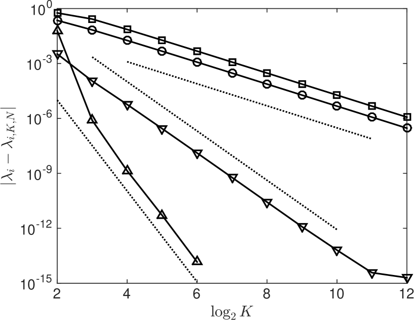
(a). $c=1/2$.

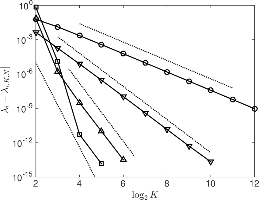
(b). $c=2/3$.

Figure 3.1. Approximation errors $|\lambda_{i}-\lambda_{i,K,N}|$ versus $K$ by the classic spectral method inspired by [29] on the unit disk. $\circ:\lambda_{1}$ ($n=0$); $\triangledown:\lambda_{2}=\lambda_{3}$ ($n=1$); $\vartriangle:\lambda_{4}=\lambda_{5}$ ($n=2$); $\square:\lambda_{6}$ ($n=0$)/$\lambda_{6}=\lambda_{7}$ ($n=3$). Dashed lines: $y=\sigma K^{-4\beta_{n}}$.

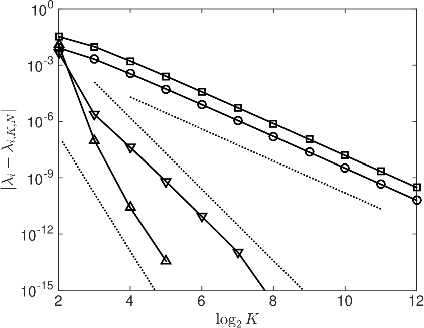
(a). $c=1/2$.

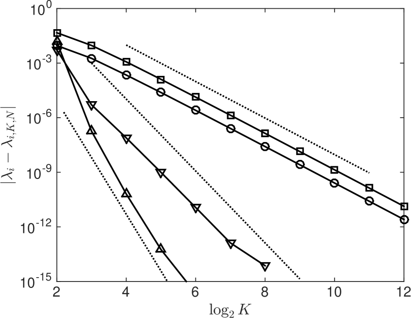
(b). $c=2/3$.

Figure 3.2. Approximation errors $|\lambda_{i}-\lambda_{i,K,N}|$ versus $K$ by the classic spectral method inspired by [29] on the unit ball. $\circ:\lambda_{1}$ ($n=0$), $\triangledown:\lambda_{2}=\lambda_{3}=\lambda_{4}$ ($n=1$), $\vartriangle:\lambda_{5}=\dots=\lambda_{9}$ ($n=2$), $\square:\lambda_{10}$ ($n=3$). Dashed lines: $y=\sigma K^{-4\beta_{n}}$.

The polynomial spectral method [27] for (1.1) utilizes the orthogonal ball polynomials as basis functions,

$$J^{-1,n+d/2-2}_{k} (2r^{2}-1)Y^{n}_{\ell}(x),$$

$$2\leq k\leq K\ \text{ if }\ c^{2}+n^{2}\neq 0,d=2\ \text{ and }\ 1\leq k\leq K\text{ if otherwise}.$$

Once again, this method leads to a series of independent algebraic eigenvalue problems with the tri-diagonal stiffness matrix and the penta-diagonal mass matrix.

The approximation errors of the polynomial spectral method are plotted in Figures 3.3 and 3.4 in log-log scale for both $c=1/2$ and $c=2/3$ in $d=2,3$ dimensions. We clearly see that the polynomial spectral method converges at a rate of $\mathcal{O}(K^{-2\beta_{n}})$, which is only the half order of the classic spectral method inspired by [29]. This even worse accuracy and convergence rate confirm the singularity of type $r^{\rho}$ of the Schrödinger eigenfunctions, which will be specified in §3.4.

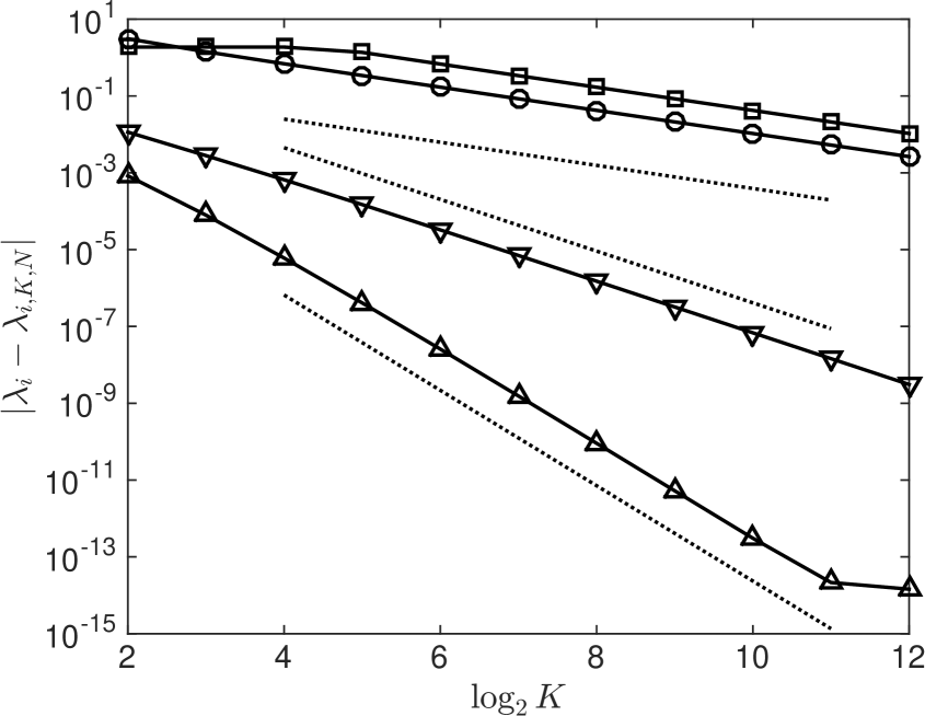
(a). $c=1/2$.

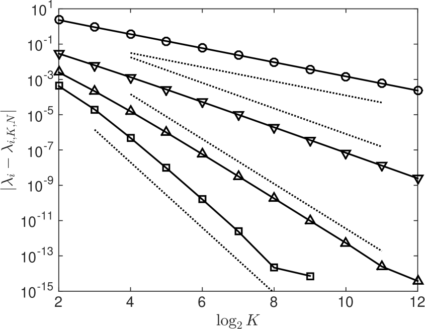
(b). $c=2/3$.

Figure 3.3. Approximation errors $|\lambda_{i}-\lambda_{i,K,N}|$ versus $K$ by the polynomial spectral method on the unit disk. $\circ:\lambda_{1}$ ($n=0$); $\triangledown:\lambda_{2}=\lambda_{3}$ ($n=1$); $\vartriangle:\lambda_{4}=\lambda_{5}$ ($n=2$); $\square:\lambda_{6}$ ($n=0$)/$\lambda_{6}=\lambda_{7}$ ($n=3$). Dashed lines: $y=\sigma K^{-2\beta_{n}}$.

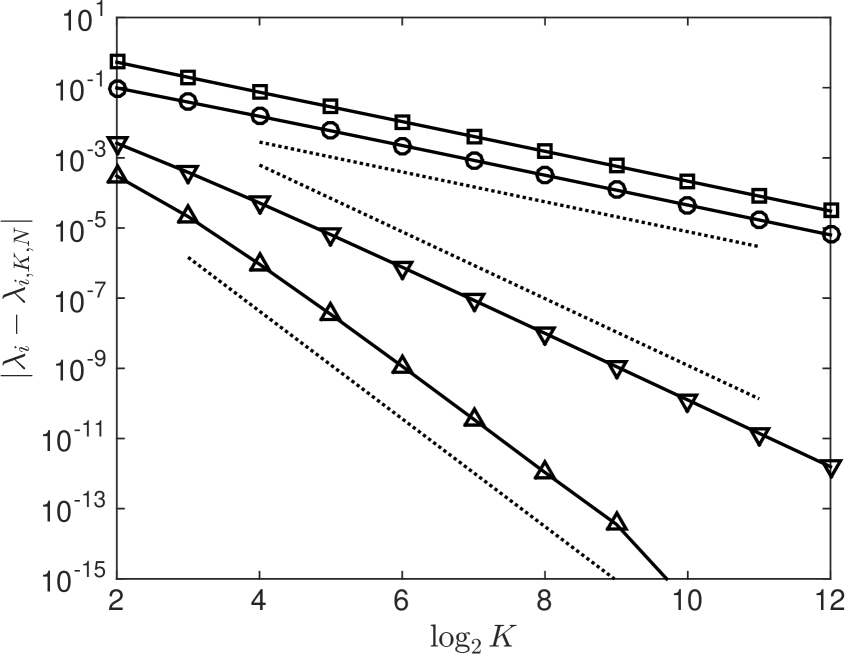
(a). $c=1/2$.

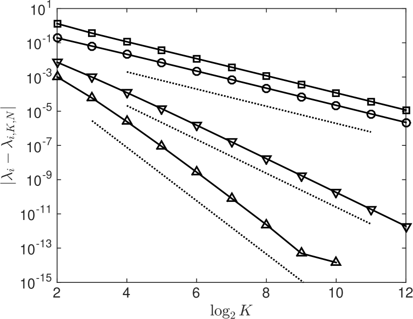
(b). $c=2/3$.

Figure 3.4. Approximation errors $|\lambda_{i}-\lambda_{i,K,N}|$ versus $K$ by the polynomial spectral method on the unit ball. $\circ:\lambda_{1}$ ($n=0$), $\triangledown:\lambda_{2}=\lambda_{3}=\lambda_{4}$ ($n=1$), $\vartriangle:\lambda_{5}=\dots=\lambda_{9}$ ($n=2$), $\square:\lambda_{10}$ ($n=3$). Dashed lines: $y=\sigma K^{-2\beta_{n}}$.

On the contrary, exponential convergence rates of our novel spectral methods are readily observed from Figures 3.5 and 3.6. These results demonstrate the effectiveness of Method I and Method II. Interestingly, the convergence order of Method II is roughly twice as high as Method I.

(a). $c=1/2$.

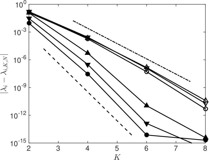
(b). $c=2/3$.

Figure 3.5. Approximation errors $|\lambda_{i}-\lambda_{i,K,N}|$ ($\circ:\lambda_{1}$, $\triangledown:\lambda_{2}=\lambda_{3}$ and $\vartriangle:\lambda_{4}=\lambda_{5}$) versus $K$ for Method I (primitive markers) and Method II (filled markers) on the unit disk. The dash-dot and dashed lines are the reference exponential $y=10^{-1.65K+4}$ and $y=10^{-3.12K+3}$, respectively.

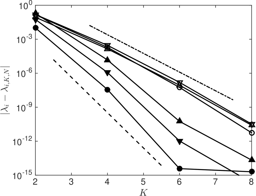
(a). $c=1/2$.

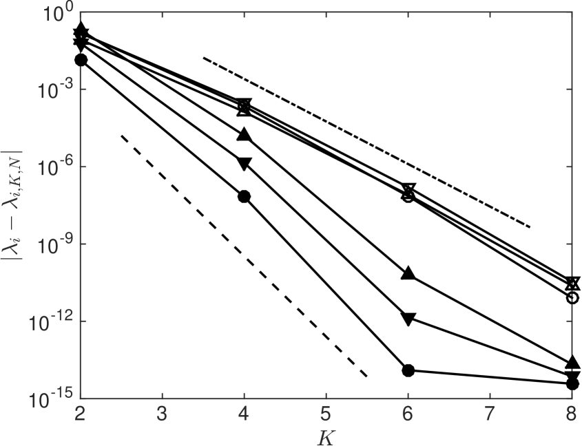
(b). $c=2/3$.

Figure 3.6. Approximation errors $|\lambda_{i}-\lambda_{i,K,N}|$ ($\circ:\lambda_{1}$, $\triangledown:\lambda_{2}=\lambda_{3}=\lambda_{4}$ and $\vartriangle:\lambda_{5}=\dots=\lambda_{9}$) versus $K$ on unit ball for Method I (primitive markers) and Method II (filled markers). The dash-dot and dashed lines are the reference exponential $y=10^{-1.65K+4}$ and $y=10^{-3.12K+3}$, respectively.

3.4. Why and how do our methods work?

We first carry out a spectral analysis on the unit ball, where the Schrödinger equation (1.1) can be reformulated, by using (2.1), in the spherical-polar coordinates as following,

(3.9) $$-\frac{1}{r^{d-1}}\partial_{r}\big{(}r^{d-1}\partial_{r}u)-\frac{1}{r^{2}}\Delta_{0}^{2}u+\frac{c^{2}}{r^{2}}u=\lambda u.$$

We now represent the unknown eigenfunction $u$ as an expansion of spherical harmonic functions,

$$u(x)=\sum_{n=0}^{\infty}\sum_{\ell=0}^{a_{n}^{d}}\widehat{u}^{n}_{\ell}(r)Y^{n}_{\ell}(\xi),\qquad x=r\xi,\,r=|x|,$$

and obtain an infinite system of second-order ordinary differential equations,

(3.10) $$-\frac{1}{r^{d-1}}\partial_{r}(r^{d-1}\partial_{r})\widehat{u}^{n}_{\ell}+\frac{c^{2}+n(n+d-2)}{r^{2}}\widehat{u}^{n}_{\ell}=\lambda\widehat{u}^{n}_{\ell},\qquad 1\leq\ell\leq a_{n}^{d},\,n\geq 0.$$

Recall that $\beta_{n}=\beta(n,c,d)=\sqrt{c^{2}+(n+d/2-1)^{2}}$, the system (3.10) is then equivalent to

$$r^{2}\partial_{r}^{2}[r^{d/2-1}\widehat{u}_{\ell}^{n}(r)]+r\partial_{r}[r^{d/2-1}\widehat{u}_{\ell}^{n}(r)]+\big{[}\lambda r^{2}-\beta_{n}^{2}\big{]}r^{d/2-1}\widehat{u}_{\ell}^{n}(r)=0,$$

Making the variable transformation $\eta=\sqrt{\lambda}\,r$ and setting $\widehat{v}^{n}_{\ell}(\eta)=r^{d/2-1}\widehat{u}^{n}_{\ell}(r)$, one obtains

$$\eta^{2}\partial_{\eta}^{2}\widehat{v}_{\ell}^{n}(\eta)+\eta\partial_{\eta}\widehat{v}_{\ell}^{n}(\eta)+\big{(}\eta^{2}-\beta_{n}^{2}\big{)}\widehat{v}_{\ell}^{n}(\eta)=0,$$

which is exactly the Sturm-Liouville equation for the first kind Bessel function, hence admits a unique solution $\widehat{v}^{n}_{\ell}(\eta)=J_{\beta_{n}}(\eta)$. In return,

(3.11) $$\widehat{u}_{\ell}^{n}(r)=r^{1-d/2}\widehat{v}_{n}(\eta)=r^{1-d/2}J_{\beta_{n}}(\sqrt{\lambda}\,r)=\sum_{m=0}^{\infty}\frac{(-1)^{m}}{m!\Gamma(m+\beta_{n}+1)}\Big{(}\frac{\sqrt{\lambda}\,{r}}{2}\Big{)}^{2m+\beta_{n}}r^{1-d/2}.$$

Since the homogeneous Dirichlet boundary condition in (2.1) implies $\widehat{u}_{\ell}^{n}(1)=0$, one readily finds that the eigenvalue $\lambda$ of (3.10) satisfies

$$J_{\beta_{n}}(\sqrt{\lambda})=0.$$

Let us now shed light on the mechanism of our methods. The terms on the left-hand side of (3.10) can be merged into one, i.e.,

$$-\frac{1}{r^{d-1}}\partial_{r}\big{(}r^{d-1}\partial_{r}\widehat{u}^{n}_{\ell})+\frac{c^{2}+n(n+d-2)}{r^{2}}\widehat{u}^{n}_{\ell}= \,-\partial_{r}^{2}\widehat{u}^{n}_{\ell}-\frac{d-1}{r}\partial_{r}\widehat{u}^{n}_{\ell}+\frac{c^{2}+n(n+d-2)}{r^{2}}\widehat{u}^{n}_{\ell}$$

$$=-\partial_{r}^{2}\widehat{u}^{n}_{\ell}-\frac{2\nu+\mu}{r}\partial_{r}\widehat{u}^{n}_{\ell}-\frac{\nu(\nu+\mu-1)}{r^{2}}\widehat{u}^{n}_{\ell}= \,-\frac{1}{r^{\mu+\nu}}\partial_{r}\Big{[}r^{\mu}\partial_{r}\big{(}r^{\nu}\widehat{u}^{n}_{\ell}\big{)}\Big{]},$$

where $\mu$ and $\nu$ are parameters to be determined by

$$2\nu+\mu=d-1,\qquad-\nu(\nu+\mu-1)=c^{2}+n(n+d-2),$$

or explicitly,

$$\nu=d/2-1\pm\beta_{n},\qquad\mu=1\mp 2\beta_{n}.$$

In particular, taking

$$-\frac{1}{r^{d-1}}\partial_{r}\big{(}r^{d-1}\partial_{r}\widehat{u}^{n}_{\ell})+\frac{c^{2}+n(n+d-2)}{r^{2}}\widehat{u}^{n}_{\ell}=-r^{-\beta_{n}-d/2}\partial_{r}\Big{[}r^{2\beta_{n}+1}\partial_{r}\big{(}r^{d/2-1-\beta_{n}}\widehat{u}^{n}_{\ell}\big{)}\Big{]},$$

one eliminates the singularity of the eigenfunction $\widehat{u}^{n}_{\ell}$ defined in (3.11) by multiplying $r^{d/2-1-\beta}$ such that the analytic function $r^{d/2-1-\beta}\widehat{u}^{n}_{\ell}(r)$ can be well approximated by the Jacobi polynomials in $r$ on $[0,1]$ with an exponential rate of convergence. This provides an explanation for the effectiveness of Method I.

As for Method II, we note that, under the modified polar-spherical coordinates $x=\sqrt{\rho}\,\xi$ with $\rho=r^{2}$,

(3.12) $$-\frac{1}{r^{d-1}}\partial_{r}\big{(}r^{d-1}\partial_{r}\widehat{u}^{n}_{\ell})+\frac{c^{2}+n(n+d-2)}{r^{2}}\widehat{u}^{n}_{\ell}=-4r^{1-d/2-\beta_{n}}\partial_{\rho}\Big{[}\rho^{\beta_{n}+1}\partial_{\rho}\big{(}r^{d/2-1-\beta_{n}}\widehat{u}^{n}_{\ell}\big{)}\Big{]}.$$

The right-side hand of (3.12) is self-adjoint with respect to the measure $r^{d-1}dr=\frac{1}{2}r^{d-2}d\rho$. According to (3.11), $r^{d/2-1-\beta_{n}}\widehat{u}^{n}_{\ell}(r)$ can be approximated by the Jacobi polynomials in $\rho=r^{2}$ on $[0,1]$ with an exponential rate of convergence. This explains the effectiveness of Method II.

4. Novel spectral method on a planar sector

In this section, we study two novel spectral methods for the Schrödinger equation on a planar circular sector, which is enclosed by the arc $\Gamma_{2}$ and two radii $\Gamma_{1}$ and $\Gamma_{3}$ (see the left of Figure 4.1):

(4.1) $$\Omega=\Lambda:= \{(r,\theta):0\leq r<1,0<\theta<\gamma^{-1}\pi\},$$

where $\gamma\geq\frac{1}{2}$, and $(r,\theta)$ is the polar coordinates satisfying $x=(r\cos\theta,r\sin\theta)$.

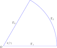
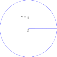
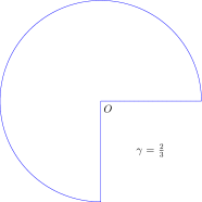
Figure 4.1. Planar circular sectors.

A heuristic idea is to expand the unknown eigenfunction $u$ by sine series

$$u(x)=\sum_{n=1}^{\infty}\widehat{u}_{n}(r)\sin(n\gamma\theta)$$

in (1.1) to obtain

$$\big{(}-\Delta +\frac{c^{2}}{r^{2}}\big{)}u(x)=\sum_{n=1}^{\infty}\left[-\frac{1}{r}\partial_{r}\big{(}r\partial_{r}\widehat{u}_{n}(r))+\frac{\beta^{2}_{n}}{r^{2}}\widehat{u}_{n}(r)\right]\sin(n\gamma\theta)$$

$$= -\sum_{n=1}^{\infty}r^{-\beta_{n}-1}\partial_{r}\Big{[}r^{2\beta_{n}+1}\partial_{r}\big{(}r^{-\beta_{n}}\widehat{u}_{n}(r)\big{)}\Big{]}\sin(n\gamma\theta),$$

where $\beta_{n}:=\beta(c,n)=\sqrt{c^{2}+\gamma^{2}n^{2}}$. This leads to the following equivalent eigen equations,

$$-r^{-\beta_{n}-1}\partial_{r}\Big{[}r^{2\beta_{n}+1}\partial_{r}\big{(}r^{-\beta_{n}}\widehat{u}_{n}(r)\big{)}\Big{]}=\lambda\widehat{u}_{n}(r),\qquad n\geq 0,$$

which motivates us to propose two types of spectral methods for (1.1) on a planar sector.

4.1. Spectral method I

We propose an approximation scheme on a circular sector in analogue to Method I in the previous section. Let us first introduce the Sobolev space

$${}_{0}W^{1}(\Lambda)=\left\{u\in W^{1}(\Lambda):u=0\text{ on }\Gamma_{1}\cup\Gamma_{3}\right\}.$$

Lemma 4.1.

Define

$$\Phi_{k}^{n}(x):=\dfrac{2k+2\beta_{n}}{k+2\beta_{n}}J_{k}^{-1,2\beta_{n}}(2r-1)r^{\beta_{n}}\sin(n\gamma\theta),\quad k\in\mathbb{N}_{0},n\in\mathbb{N}.$$

Then $\Phi_{k}^{n}(x),\,k\in\mathbb{N}_{0},\,n\in\mathbb{N}$ form a Sobolev orthogonal basis in ${}_{0}W^{1}(\Lambda)$ in the following sense,

$$(\nabla\Phi_{k}^{n},\nabla\Phi_{j}^{m})_{\Lambda}+c^{2}(\Phi_{k}^{n},\Phi_{j}^{m})_{r^{-2},\Lambda}=\frac{\pi}{2\gamma}\delta_{m,n}\delta_{j,k}(k+\beta_{n})(2-\delta_{k,0}).$$

Moreover,

$$(\Phi_{k}^{n},\Phi_{j}^{m})_{\Lambda}=\, \frac{\pi}{2\gamma}\delta_{n,m}\times\begin{cases}\frac{(k+\beta_{n})(k^{2}+2k\beta_{n}+4\beta_{n}^{2}-1)}{(k+\beta_{n}-1)(k+\beta_{n}+1)(2k+2\beta_{n}-1)(2k+2\beta_{n}+1)},&k=j\geq 1,\\[3.00003pt] \frac{1}{2(\beta_{n}+1)},&k=j=0,\\[3.00003pt] -\frac{(2\beta_{n}-1)(2\beta_{n}+1)}{(2k+2\beta_{n}-1)(2k+2\beta_{n}+1)(2k+2\beta_{n}+3)},&j=k+1,\\[3.00003pt] -{\frac{(k+1)(k+2\beta_{n}+1)}{2(k+\beta_{n}+1)(2k+2\beta_{n}+1)(2k+2\beta_{n}+3)}},&j=k+2,\\[3.00003pt] -\frac{(2\beta_{n}-1)(2\beta_{n}+1)}{(2j+2\beta_{n}-1)(2j+2\beta_{n}+1)(2j+2\beta_{n}+3)},&k=j+1,\\[3.00003pt] -{\frac{(j+1)(j+2\beta_{n}+1)}{2(j+\beta_{n}+1)(2j+2\beta_{n}+1)(2j+2\beta_{n}+3)}},&k=j+2,\\[3.00003pt] 0,&\text{otherwise}.\end{cases}$$

Lemma 4.1 can be proved similarly as Lemma 3.1, we omit the details.

Define the approximation space

$$W_{K,N}^{\Lambda}=\left\{\Phi_{k}^{n}:1\leq k\leq K,\,0\leq n\leq N\right\}\subset W^{1}_{0}(\Lambda).$$

Then the spectral-Galerkin approximation scheme is, to find $u_{K,N}\in W_{K,N}^{\Lambda}$ such that

$$a(u_{K,N},v)=(\nabla u_{K,N},\nabla v)_{\Lambda}+c^{2}(u_{K,N},v)_{r^{-2},{\Lambda}}=\lambda_{K,N}(u_{K,N},v)_{\Lambda},\qquad v\in W_{K,N}^{\Lambda}.$$

It is worthy to note that this approximation scheme leads to an algebraic eigen system with a diagonal stiffness matrix and a penta-diagonal mass matrix, which can be easily decoupled and solved in parallel.

4.2. Spectral method II

Our second method for (1.1) on a circular sector is based on the following lemma, which is an analogue to Lemma 3.2.

Lemma 4.2.

Define

$$\Psi_{k}^{n}(x):=\dfrac{2k+\beta_{n}}{k+\beta_{n}}J_{k}^{-1,\beta_{n}}(2r^{2}-1)r^{\beta_{n}}\sin(n\gamma\theta),\quad k\in\mathbb{N}_{0},\,n\in\mathbb{N}.$$

Then $\Psi_{k}^{n}(x),\,k\in\mathbb{N}_{0},\,n\in\mathbb{N}$ form a Sobolev orthogonal basis in ${}_{0}W^{1}(\Lambda)$ in the following sense,

$$(\nabla \Psi_{k}^{n},\nabla\Psi_{j}^{m})_{\Lambda}+c^{2}(\Psi_{k}^{n},\Psi_{j}^{m})_{r^{-2},{\Lambda}}=\frac{\pi}{2\gamma}\delta_{m,n}\delta_{k,j}(2k+\beta_{n})(2-\delta_{k,0}).$$

Moreover,

$$(\Psi_{k}^{n},\Psi_{j}^{m})_{\Lambda}:=\, \frac{\pi}{2\gamma}\delta_{n,m}\times\begin{cases}\frac{1}{2k+\beta_{n}+1}+\frac{1-\delta_{k,0}}{2k+\beta_{n}-1},&k=j,\\ -\frac{1}{2(2k+\beta_{n}+1)},&j=k+1,\\ -\frac{1}{2(2j+\beta_{n}+1)},&k=j+1,\\ 0,&\text{otherwise}.\end{cases}$$

We omit the proof, which is similar to that of Lemma 3.2 as in the Appendix A.

Define the approximation space

$$V_{K,N}^{\Lambda}=\left\{\Psi_{k}^{n}:1\leq k\leq K,\,0\leq n\leq N\right\}\subset W^{1}_{0}(\Lambda).$$

Then the spectral-Galerkin approximation scheme is, to find $u_{K,N}\in V_{K,N}^{\Lambda}$ such that

$$a(u_{K,N},v)=(\nabla u_{K,N},\nabla v)_{\Lambda}+c^{2}(u_{K,N},v)_{r^{-2},{\Lambda}}=\lambda_{K,N}(u_{K,N},v)_{\Lambda},\qquad v\in V_{K,N}^{\Lambda}.$$

This approximation scheme leads to an algebraic eigen system with a diagonal stiffness matrix and a tridiagonal mass matrix, which can also be decoupled easily and solved in parallel.

4.3. Numerical experiments

Our novel spectral methods for (1.1) are examined on the slit disk ($\gamma=\frac{1}{2}$) and the circular sector with $\gamma=\frac{2}{3}$. The approximation errors of the 3 smallest eigenvalues are reported in Figure 4.2 in semi-log scale. The exponential convergence is observed for both Method I and Method II. Furthermore, a comparison of Figure 4.2 with Figures 3.5-3.6 reveals that both Method I and Method II converge at a fixed order of their own regardless of $\Omega$ being a ball or a circular sector. Finally, since the radial component of the eigenfunction $r^{-\beta_{n}}\widehat{u}_{n}(r)$ is analytic in $\rho=r^{2}$, Method II nearly converges twice as fast as Method I, just as shown in Figure 4.2.

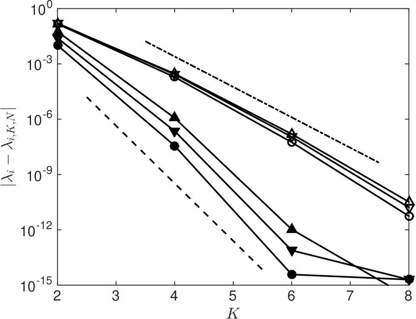
(a). $\gamma=1/2,\,c=1/2$.

(b). $\gamma=1/2,\,c=2/3$.

(c). $\gamma=2/3,\,c=1/2$.

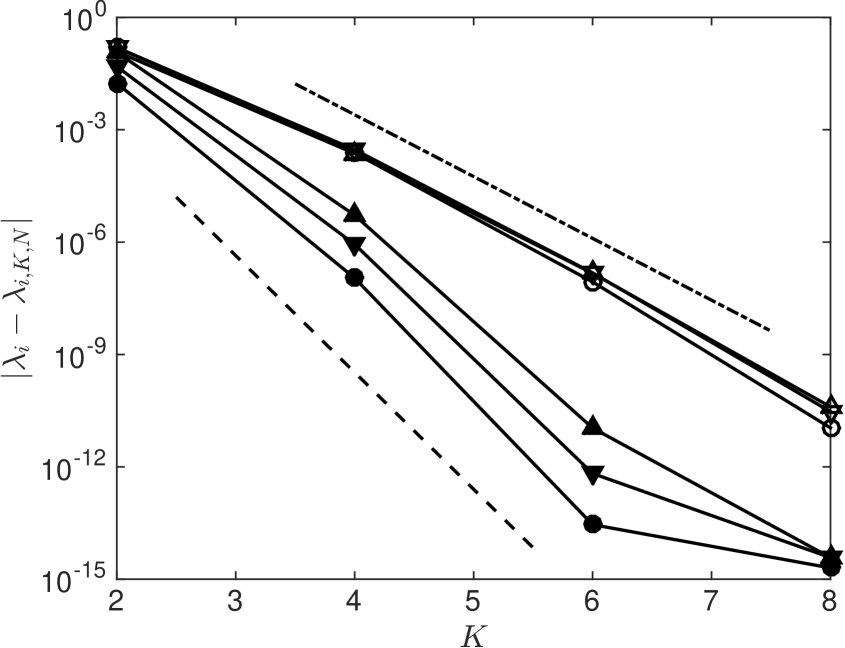
(d). $\gamma=2/3,\,c=2/3$.

Figure 4.2. Approximation errors $|\lambda_{i}-\lambda_{i,K,N}|$ ($\circ:\lambda_{1}$, $\triangledown:\lambda_{2}$ and $\vartriangle:\lambda_{3}$) versus $K$ on the circular sectors. Method I (primitive markers) and Method II (filled markers). The dash-dot and dashed lines are the reference exponential $y=10^{-1.65K+4}$ and $y=10^{-3.12K+3}$, respectively.

5. Mortar spectral element methods

The mortar element method uses nonconforming domain decomposition technique, which allows to choose independently the discretization method on each sub-domain to adapt to the local behavior of the partial differential equation [3, 7]. For simplicity, we consider only mortar spectral element methods on planar domains.

5.1. Mortar spectral elements on a regular domain

Let $\Omega$ be a bounded domain $\mathbb{R}^{2}$ such that $(0,0)\in\Omega$ and $(0,0)\notin\partial\Omega$. We first use the circle centered at the original with the radius $R>0$,

$$\Gamma_{R}=\left\{(x,y)=(R\cos\theta,R\sin\theta):0\leq\theta\leq 2\pi\right\}\subset\Omega\setminus\partial\Omega,$$

to decompose $\Omega$ into two subdomains

$$\Omega_{0}=\{(x,y)\in\mathbb{R}^{2}:x^{2}+y^{2}<R^{2}\},\quad\Omega_{1}=\Omega\setminus\Omega_{0}.$$

For discretization, our main idea is to use a novel spectral method on the disk $\Omega_{0}$ while use the standard spectral element method on $\Omega_{1}$.

Let us take $\Omega=[-1,1]^{2}$ as an example to explain our idea. For simplicity, we further decompose $\Omega_{1}$ into four curvilinear quadrilaterals by the two diagonals of the square as indicated in the left side of Figure 5.1,

$$\Omega_{1}^{(1)}=\{(x,y)\in\mathbb{R}^{2}:x^{2}+y^{2}>R^{2},\,|y|<x<1\},$$

$$\Omega_{1}^{(2)}=\{(x,y)\in\mathbb{R}^{2}:x^{2}+y^{2}>R^{2},\,|x|<y<1\},$$

$$\Omega_{1}^{(3)}=\{(x,y)\in\mathbb{R}^{2}:x^{2}+y^{2}>R^{2},\,|y|<-x<1\},$$

$$\Omega_{1}^{(4)}=\{(x,y)\in\mathbb{R}^{2}:x^{2}+y^{2}>R^{2},\,|x|<-y<1\}.$$

In such a way, we have the non-overlapping partition $\Omega=\Omega_{0}\cup\Omega_{1}^{(1)}\cup\Omega_{1}^{(2)}\cup\Omega_{1}^{(3)}\cup\Omega_{1}^{(4)}$, and the interior edges of each $\Omega_{1}^{(\kappa)}$ ($1\leq\kappa\leq 4$) are then perpendicular to the circle.

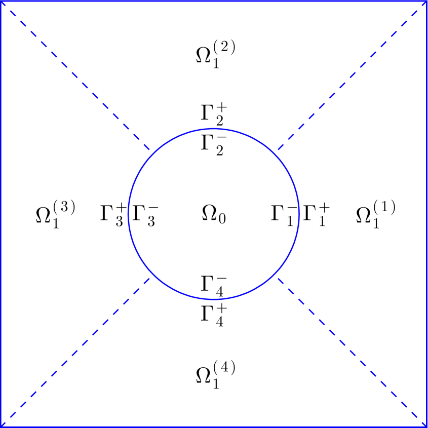
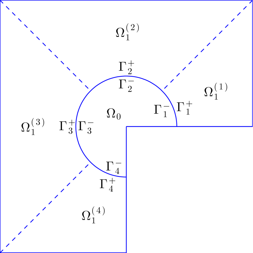
Figure 5.1. Non-conforming meshes for the mortar spectral method on a square (left) and an L-shape domain (right).

We now introduce the approximation space. Denote $\delta=(K_{0},N_{0},K_{1},N_{1})$. Let $T_{0}:\mathbb{B}^{2}\mapsto\Omega_{0}$ such that $(x,y)=T_{0}(\xi,\eta)=(R\xi,R\eta)$, and define the approximation space on $\Omega_{0}$,

$$X_{\delta,0}=\operatorname{span}\big{\{}P_{k,\ell}^{n}\circ T_{0}^{-1}:0\leq k\leq K_{0},\,1\leq\ell\leq a_{n}^{2},\,0\leq n\leq N_{0}\big{\}}.$$

To introduce the approximation space on $\Omega_{1}$, we first make the Gordon-Hall transformations $T_{\kappa}:[-1,1]^{2}\mapsto\Omega_{1}^{(\kappa)}$, $\kappa=1,2,3,4$, such that

$$(x+\i y)=\i^{\kappa-1}\left[\frac{1+\xi}{2}(1+\i\eta)+\frac{1-\xi}{2}R\mathrm{e}^{\frac{\i\pi\eta}{4}}\right],$$

or equivalently,

(5.1) $$\begin{cases}x=\dfrac{1+\xi}{2}\left[\sin\dfrac{\pi\kappa}{2}+\eta\cos\dfrac{\pi\kappa}{2}\right]+\dfrac{1-\xi}{2}R\sin\dfrac{\pi(\eta+2\kappa)}{4},\\[5.0pt] y=\dfrac{1+\xi}{2}\left[\eta\sin\dfrac{\pi\kappa}{2}-\cos\dfrac{\pi\kappa}{2}\right]-\dfrac{1-\xi}{2}R\cos\dfrac{\pi(\eta+2\kappa)}{4}.\end{cases}$$

Then we define the conforming approximation space on $\Omega_{1}$ as following,

$$X_{\delta,1}=\operatorname{span}\big{\{}v\in H^{1}(\Omega_{1}):v|_{\Omega_{1}^{(\kappa)}}\circ T_{\kappa}\in X_{K_{1},N_{1}},\kappa=1,2,3,4\big{\}},$$

$$X_{K_{1},N_{1}}=\operatorname{span}\left\{v\in\mathbb{P}_{K_{1}}\times\mathbb{P}_{N_{1}}:v(1,\eta)=0\right\}.$$

Finally, our mortar approximation space on $\Omega$ is defined by

$$X_{\delta}=\operatorname{span}\left\{v:v|_{\Omega_{i}}\in X_{\delta,i},i=0,1;\quad(\gamma^{-}v-\gamma^{+}v,\phi)_{\Gamma_{R}}=0,\quad\phi\in V_{\delta}\right\},$$

where the non mortar space $V_{\delta}$ is defined through either the trace operator $\gamma^{+}:X_{\delta,1}\mapsto L^{2}(\Gamma_{R})$ or $\gamma^{-}:X_{\delta,0}\mapsto L^{2}(\Gamma_{R})$, i.e., $V_{\delta}\subseteq\{\gamma^{+}v_{\delta}:v_{\delta}\in X_{\delta,1}\}$ or $V_{\delta}\subseteq\{\gamma^{-}v_{\delta}:v_{\delta}\in X_{\delta,0}\}$. Note that the matching condition $(\gamma^{-}v-\gamma^{+}v,\phi)_{\Gamma_{R}}=0,\ \phi\in V_{\delta}$ is enforced to guarantee information interchange between $X_{\delta,1}$ and $X_{\delta,0}$, and here we simply use

$$V_{\delta}=\operatorname{span}\{\gamma^{-}v_{\delta}:v_{\delta}\in X_{\delta,0}\}=\operatorname{span}\left\{\mathrm{e}^{\i n\theta}:-N_{0}\leq n\leq N_{0}\right\}.$$

The mortar spectral element approximation scheme reads: Find the eigenpairs $(\lambda_{\delta},u_{\delta})\in\mathbb{R}_{+}\times X_{\delta}$ such that

(5.2) $$(\nabla u_{\delta},\nabla v_{\delta})_{\Omega}+(u_{\delta},v_{\delta})_{r^{-2},\Omega}=\lambda_{\delta}(u_{\delta},v_{\delta})_{\Omega},\quad v_{\delta}\in X_{\delta}.$$

If we remove the matching condition in the definition of $X_{\delta}$ to obtain

$$X_{\delta}^{*}=\left\{v:v|_{\Omega_{i}}\in X_{\delta,i},i=0,1\right\},$$

then (5.2) is equivalent to the following one: Find $(\lambda_{\delta},u_{\delta},\psi_{\delta})\in\mathbb{R}_{+}\times X_{\delta}^{*}\times V_{\delta}$ such that

(5.3) $$\begin{split}&(\nabla u_{\delta},\nabla v_{\delta})_{\Omega}+(u_{\delta},v_{\delta})_{r^{-2},\Omega}+(\gamma^{-}v_{\delta}-\gamma^{+}v_{\delta},\psi_{\delta})_{\Gamma_{R}}=\lambda_{\delta}(u_{\delta},v_{\delta})_{\Omega},\quad v_{\delta}\in X_{\delta}^{*},\\ &(\gamma^{-}u_{\delta}-\gamma^{+}u_{\delta},\phi_{\delta})_{\Gamma_{R}}=0,\quad\phi_{\delta}\in V_{\delta}.\end{split}$$

Before concluding this subsection, we give some remarks on the evaluation of the matrices of the reduced algebraic problems in our mortar spectral element method. The local stiffness matrix associating $(\nabla\cdot,\nabla\cdot)_{\Omega_{0}}+(\cdot,\cdot)_{r^{-2},\Omega_{0}}$ and the local mass matrix associating $(\cdot,\cdot)_{\Omega_{0}}$ can be easily obtained from Lemma 3.2. While for the local stiffness and mass matrices on $\Omega_{1}^{(\kappa)},\,(1\leq\kappa\leq 4)$, we only need to consider the local matrices on $\Omega_{1}^{(1)}$ owing to the parity of our symmetric partition. We first use the following basis functions for $X_{K_{1},N_{1}}$,

$$X_{K_{1},N_{1}}=\left\{\phi_{k,n}(\xi,\eta):=\phi_{k}(\xi)\phi_{n}(\eta):0\leq k\leq K_{1},1\leq n\leq N_{1}\right\},$$

where

$$\phi_{0}(\zeta)=\frac{1+\zeta}{2},\ \phi_{1}(\zeta)=\frac{1-\zeta}{2},\quad\phi_{k}(\zeta)=J^{-1,-1}_{k}(\zeta),\ k\geq 2.$$

Next, we note that the following differentiation relation under the Gordon-Hall mapping $T_{1}$,

$$\widetilde{\nabla}:=\begin{bmatrix}\partial_{\xi}\\ \partial_{\eta}\end{bmatrix}=J_{1}\begin{bmatrix}\partial_{x}\\ \partial_{y}\end{bmatrix}=J_{1}\nabla,\qquad\nabla=\begin{bmatrix}\partial_{x}\\ \partial_{y}\end{bmatrix}=J_{1}^{-1}\begin{bmatrix}\partial_{\xi}\\ \partial_{\eta}\end{bmatrix}=J_{1}^{-1}\widetilde{\nabla},$$

where

$$J_{1}=\begin{bmatrix}\frac{1}{2}-\frac{R}{2}\cos\frac{\pi\eta}{4}&\frac{\eta}{2}-\frac{R}{2}\sin\frac{\pi\eta}{4}\\[5.0pt] \frac{\pi}{8}(\xi-1)R\sin\frac{\pi\eta}{4}&\frac{\xi+1}{2}-\frac{\pi}{8}(\xi-1)R\cos\frac{\pi\eta}{4}\end{bmatrix},$$

$$|J_{1}|=\det(J_{1})=-\frac{(\pi+4)\xi+(4-\pi)}{16}R\cos\frac{\pi\eta}{4}-\frac{\pi\eta(\xi-1)}{16}R\sin\frac{\pi\eta}{4}+\frac{\xi+1}{4}+\frac{R^{2}\pi(\xi-1)}{16}.$$

Then the local mass matrix on $\Omega_{1}^{(1)}$ can be precisely expressed by Bessel functions, while each entry of local stiffness matrix can be easily evaluated through the Gaussian quadratures on $[-1,1]^{2}$. Moreover, since $\phi_{k,n}(-1,\eta)=\delta_{k,0}\phi_{n}(\eta)$, one readily finds that the matrix relating to the mortar elements on $\Gamma_{R}$ can also be formulated explicitly using Bessel functions.

5.2. Mortar spectral elements on a domain with reentrant corners

For simplicity, let us consider the L-shape domain and suppose $\Omega=[-1,1]^{2}\setminus([0,1]\times[-1,0])$ such that the point of the potential singularity is also the vertex of the reentrant corner. The computational domain $\Omega$ is partitioned using the same technique as in the previous subsection. More precisely, $\Omega=\Omega_{0}\cup\Omega_{1}$, $\Omega_{1}=\Omega_{1}^{(1)}\cup\Omega_{1}^{(2)}\cup\Omega_{1}^{(3)}\cup\Omega_{1}^{(4)}$, and

$$\Gamma_{R}=\{(x,y)=(R\cos\theta,R\sin\theta):0\leq\theta\leq\frac{3\pi}{2}\}\subset\Omega,$$

$$\Omega_{0}=\{(x,y)=(r\cos\theta,r\sin\theta):0\leq r<R,\,0\leq\theta\leq\frac{3\pi}{2}\},$$

$$\Omega_{1}^{(1)}=\{(x,y)\in\mathbb{R}^{2}:x^{2}+y^{2}>R^{2},\,0<y<x<1\},$$

$$\Omega_{1}^{(2)}=\{(x,y)\in\mathbb{R}^{2}:x^{2}+y^{2}>R^{2},\,|x|<y<1\},$$

$$\Omega_{1}^{(3)}=\{(x,y)\in\mathbb{R}^{2}:x^{2}+y^{2}>R^{2},\,-1<x<-|y|\},$$

$$\Omega_{1}^{(4)}=\{(x,y)\in\mathbb{R}^{2}:x^{2}+y^{2}>R^{2},\,-1<y<x<0\}.$$

The Gordon-Hall mappings $T_{\kappa}:[-1,1]^{2}\mapsto\Omega_{1}^{(\kappa)}$ are the same as in (5.1) for $\kappa=2,3$ and are defined as following for $\kappa=1,4$,

$$F_{1}:\quad\begin{cases}x=\tfrac{1+\xi}{2}+\tfrac{1-\xi}{2}R\cos\frac{\pi(\eta+1)}{8},\\ y=\tfrac{1+\xi}{2}\tfrac{1+\eta}{2}+\tfrac{1-\xi}{2}R\sin\frac{\pi(\eta+1)}{8},\end{cases}$$

$$F_{4}:\quad\begin{cases}x=-\tfrac{1+\xi}{2}\tfrac{1+\eta}{2}-\tfrac{1-\xi}{2}R\sin\frac{\pi(\eta+1)}{8},\\ y=-\tfrac{1+\xi}{2}-\tfrac{1-\xi}{2}R\cos\frac{\pi(\eta+1)}{8}.\end{cases}$$

Denote $\delta=(K_{0},N_{0},K_{1},N_{1},K_{2},N_{2},K_{3},N_{4},K_{4},N_{4})$ and let $T_{0}:\mathbb{B}^{2}\mapsto\Omega_{0}$ be the same as in the former subsection. We now define the approximation spaces on $\Omega_{0}$ and $\Omega_{1}$,

$$X_{\delta,0}=\left\{v:v\circ T_{0}\in V_{K_{0},N_{0}}^{\Lambda}\right\}=\operatorname{span}\big{\{}\Psi_{k}^{n}\circ T_{0}^{-1}:1\leq k\leq K_{0},\,0\leq n\leq N_{0}\big{\}}.$$

and

$$X_{\delta,1}=\operatorname{span}\big{\{}v\in H^{1}(\Omega_{1}):v|_{\Omega_{1}^{(\kappa)}}\circ T^{-1}_{\kappa}\in X_{K_{\kappa},N_{\kappa}},\kappa=1,2,3,4\big{\}},$$

$$X_{K_{\kappa},N_{\kappa}}=\operatorname{span}\left\{v\in\mathbb{P}_{K_{\kappa}}\times\mathbb{P}_{N_{\kappa}}:v(1,\eta)=0\right\}.$$

Our mortar approximation space on $\Omega$ is defined again by

$$X_{\delta}=\operatorname{span}\left\{v:v|_{\Omega_{i}}\in X_{\delta,i},i=0,1;\quad(\gamma^{-}v-\gamma^{+}v,\phi)_{\Gamma_{R}}=0,\quad\phi\in V_{\delta}\right\},$$

where the non mortar space $V_{\delta}$ is chosen as

$$V_{\delta}=\operatorname{span}\{\gamma^{+}v_{\delta}:v_{\delta}\in X_{\delta,1}\}$$

to ensure a spectrally high approximation accuracy on the $\Gamma_{R}$.

Now the mortar spectral element approximation scheme for (1.1) on the L-shape domain with a singular corner exactly follows the formulas (5.2) and (5.3).

At last, we conclude this subsection with the remark that one can readily extend our mortar spectral element method to solve (1.1) with multiple singular potentials and reentrant/obtuse corners.

5.3. Numerical experiments

In this subsection, we shall show some numerical results on the mortar spectral element method (MSEM) for (1.1). To evaluate our method, we first introduce the $hp$-finite element method using geometric mesh (GFEM) by Gui, Guo and Babuška [18, 2] to handle corner/polar singularity of type $r^{\alpha}$ in numerical PDE. This method offers the best (exponential) convergence rate among traditional methods for handling such kind of singularities. The geometric mesh is characterized by $n$ layers of conforming elements, in which the size of elements in the $i$-th layer, $h_{i}=cq^{n-i},\,0<q<1,\,1\leq i\leq n$, and the polynomial degree of elements in the $i$-th layer, $p_{i}$, is proportional to its layer number $i$. In such a way, the mesh is refined as $n$ increases and simultaneously the degrees of elements are increased too.

Figure 5.2. The geometric meshes around the original on the square $\Omega=[-1,1]^{2}$ with the mesh level $n=1$ (left), $n=3$ (center) and on the L-shape domain $\Omega=[-1,1]^{2}\setminus([0,1]\times[-1,0])$ with the mesh level $n=7$ (right).

Example 1

We first examine the Schrödinger equation (1.1) on $[-1,1]^{2}$ with $c=1/2$ and $c=2/3$. The reference eigenvalues are evaluated by GFEM with $n=17$, $q=(\sqrt{2}-1)^{2}$ and $p_{i}=i,\,1\leq i\leq n$, to obtain a 15-digit precision with an optimal convergence order [18]. Numerical eigenvalues of MSEM are computed with the parameters $R=0.3$ and $\delta=(10,14,17,18)$, whose absolute errors are reported in the fourth columns of Table 5.1 and Table 5.2. It can be easily observed that the error of the MSEM with the total degrees of freedom (DoF) $1539$ is close to the machine precision, which reflect the spectral accuracy of our MSEM method.

In comparison, we also introduce a spectral element method (SEM) with four rectangular subdomains with the common vertex at the original. This method is proposed from the standard spectral element method by enforcing the vanishing of all the basis functions at the original, hence is equivalent to the reduced GFEM with $n=1$. Errors with the (separate) polynomial degree $p=61$ are then listed in the fifth columns of Table 5.1 and Table 5.2, where an obviously low accuracy is found, especially for the first and the fifth smallest eigenvalues. This indicates only a limited low order of convergence rate can be obtained in a classic spectral element discretization.

To take an insight of the superiority of MSEM to GFEM, we further present in the last columns of Table 5.1 and Table 5.2 the approximation errors of GFEM using a slightly larger degrees of freedom. It is obvious that our MSEM acquires an accuracy at least 6-digit higher than GFEM. Quantitatively, let us compare the error plots of the 4 smallest MSEM eigenvalues (i.e., $|\lambda_{i}-\lambda_{i,\delta}|$ versus $\sqrt{DoF}$ in a semi logarithm scale) in Figure 5.3 with the error plots of the GFEM eigenvalues (i.e., $|\lambda_{i}-\lambda_{i,\delta}|$ versus $\sqrt[3]{DoF}$) in Figure 5.4. The plots reveal that MSEM converges asymptotically in $\mathcal{O}\big{(}\exp({-\sigma_{1}\sqrt{DoF}})\big{)}$ while GFEM converges only in $\mathcal{O}\big{(}\exp({-\sigma_{2}\sqrt[3]{DoF}})\big{)}$ with $\sigma_{2}$ varying from case to case. More importantly, using generic local basis functions in the function space which the eigenfunctions belong to, MSEM characterizes the underlying singularities perfectly and approximates consecutive eigenvalues (together with the corresponding eigenfunctions) with an almost uniform convergence rate. While GFEM mimics the singular solution by a balance between local mesh sizes and local polynomial degrees, and can only remove part of the singularities. Thus it approximates consecutive eigenvalues with different convergence rates whenever their associate eigenfunctions possess different orders of singularities.

Table 5.1. The reference values of the first 6 eigenvalues on $[-1,1]^{2}$ for $c=1/2$; the errors of MSEM with $DoF=1539$, of SEM with $DoF=14640$, and of the GFEM with $n=8$ and $DoF=1624$.

No.	Ref.	Mul.	MSEM	SEM	GFEM
1	8.37681498711058	1	5.3291e-15	1.1417e-03	7.9985e-6
2	13.35313963139164	2	8.8818e-15	2.7979e-08	6.4234e-9
3	20.33106215893244	1	3.5527e-15	2.4869e-14	3.3054e-8
4	25.42501776089188	1	4.9738e-14	1.8474e-13	1.8657e-8
5	30.86901223422695	1	3.3040e-13	3.3095e-03	2.2988e-5
6	32.83995595781530	2	3.5527e-14	2.6943e-08	1.2435e-5

Table 5.2. The reference values of the first 6 eigenvalues on $[-1,1]^{2}$ for $c=2/3$; the errors of MSEM with $DoF=1539$, of SEM with $DoF=14640$, and of GFEM with $n=8$ and $DoF=1624$.

No.	Ref.	Mul.	MSEM	SEM	GFEM
1	9.65231567885163	1	1.7764e-15	8.9349e-5	2.4365e-7
2	14.0914338712714	2	1.0658e-14	3.1005e-8	1.1318e-8
3	20.7838715370525	1	2.4869e-14	7.8160e-14	3.5321e-8
4	25.9999831911128	1	7.1054e-14	6.7502e-14	2.1666e-8
5	32.8581767543383	1	7.8160e-14	2.7518e-04	8.0361e-7
6	33.3937111616692	2	1.4211e-14	2.9763e-08	1.5920e-6

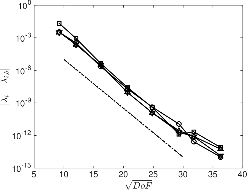
(a). $c=1/2$.

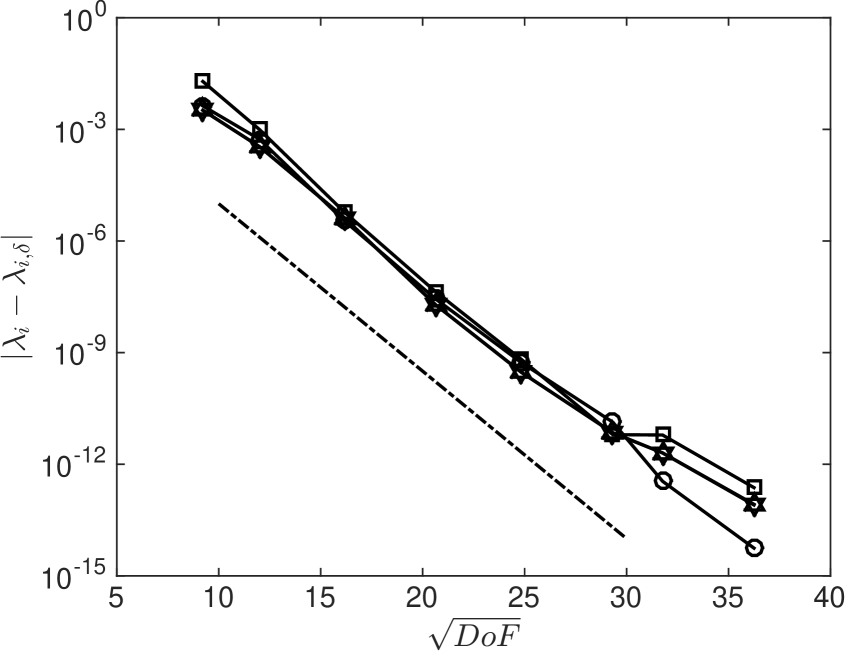
(b). $c=2/3$.

Figure 5.3. MSEM approximation errors $|\lambda_{i}-\lambda_{i,\delta}|$ ($\circ:\lambda_{1}$, $\triangledown:\lambda_{2}$, $\vartriangle:\lambda_{3}$ and $\square:\lambda_{4}$) versus $\sqrt{DoF}$ on the square $[-1,1]^{2}$. The dash-dot lines are the reference exponential $y=10^{-0.45\sqrt{DoF}-0.5}$.

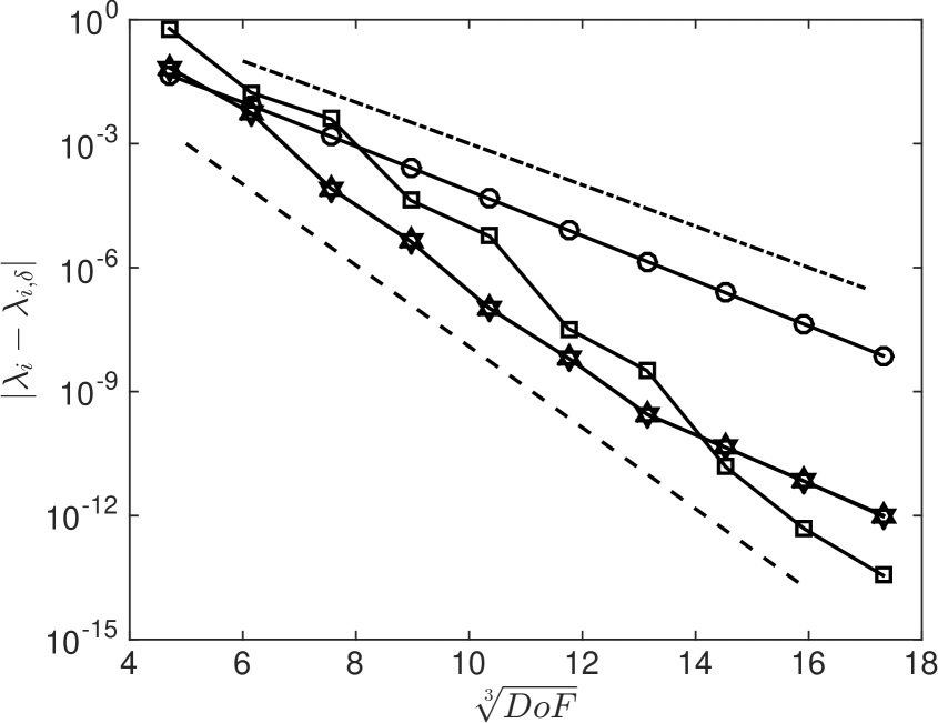
(a). $c=1/2$.

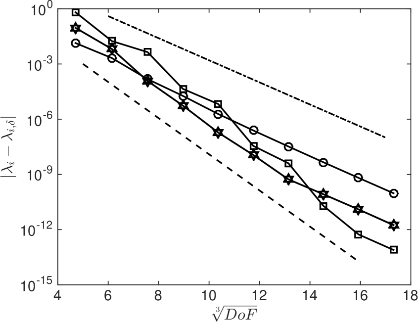
(b). $c=2/3$.

Figure 5.4. GFEM approximation errors $|\lambda_{i}-\lambda_{i,\delta}|$ ($\circ:\lambda_{1}$, $\triangledown:\lambda_{2}$, $\vartriangle:\lambda_{3}$ and $\square:\lambda_{4}$) versus $\sqrt[3]{DoF}$ on the square $[-1,1]^{2}$. The dashed lines are $y=10^{-0.98\sqrt[3]{DoF}+1.9}$; the dash-dot lines are (a). $y=10^{-0.5\sqrt[3]{DoF}+2}$ and (b). $y=10^{-0.6\sqrt[3]{DoF}+3}$.

Example 2

Further, let us examine the MSEM for solving (1.1) on the L-shape domain. Once again, the reference eigenvalues are given by the GFEM using a $17$-level geometric mesh with $q=(\sqrt{2}-1)^{2}$ and $p_{i}=i$ on each subdomain of level $i$, which amounts to a high degrees of freedom $10552$. In Table 5.3, absolute errors (for $c=0$) are given in the third column for the MSEM eigenvalues, which are evaluated using the discretization parameters $R=0.5$ and $\delta=(\{17,20\},\{15,9\},\{15,18\}^{2},\{15,9\})$ with the total degrees of freedom $1152$. As a comparison, approximation errors for SEM (GFEM with $n=1$ and $p=64$) with the degrees of freedom $12033$ and GFEM ($n=8$) with the degree of freedom $1182$ are listed in the subsequent columns, respectively. The defect of the SEM for (1.1) on the L-shape domain is as obvious as before; while the difference in error between the GFEM and our MSEM is astonishing, and MSEM is several-digit superior to GFEM in accuracy.

Moreover, we utilize the MATLAB code of the modified method of particular solution (MMPS) provided by Betcke and Trefethen [4] for solving the Laplacian eigenvalue problem on the L-shape domain with $N=72$ particular solutions (trial functions), $2N$ equally distributed boundary points and $2N$ randomly distributed interior points. Approximation errors are then reported in the last column. This shows that our MSEM is also superior to MMPS for small eigenvalues, although the latter is specifically designed for evaluating Laplacian eigenvalues on a polygon domain with reentrant corners.

To have a fair comparison, a few issues need to be addressed. The method of particular solution (MPS) starts with various solutions of the eigenvalue equation for a given $\lambda$, and then vary $\lambda$ until one can find a linear combination of such solutions that satisfies the boundary condition at a number of sample points along the boundary. improves/revives MPS (mainly in stability) by restricting the set of admissible functions to functions that are bounded away from zero in the interior. In practice this idea is realized by minimizing the angle $\phi(\lambda)$ between the space of functions that satisfy the eigenvalue equation and the space of functions that are zero on the boundary. The advantage of MMPS is that it can acquire an exponential rate of convergence by using a small number of trial functions. However, its convergence can not always be guaranteed due to its nearly singular matrix resulted. Futhermore, MMPS is not capable of distinguishing multiple eigenvalues from simple eigenvalues. More importantly, targetting at eigenvalue problems, MMPS can not be directly applicable for solving source problems as freely as our variationaly formulated methods.

Once again, we plot the absolute errors in Figure 5.5 and Figure 5.6 which clearly show that MSEM converges asymptotically in $\mathcal{O}\big{(}\exp({-\sigma_{1}\sqrt{DoF}})\big{)}$ while GFEM converges only in $\mathcal{O}\big{(}\exp({-\sigma_{2}\sqrt[3]{DoF}})\big{)}$ with $\sigma_{2}$ varying possibly from case to case. One readily observes that the convergence rates of MSEM for consecutive eigenvalues are almost uniform, while the convergence rate of GFEM varies depending on the singularities of the corresponding eigenfunctions. These phenomenon confirm the superiority of MSEM to GFEM.

Table 5.3. Reference values (column 2) of the first 10 Dirichlet Laplacian eigenvalues on $[-1,1]^{2}\setminus([0,1]\times[-1,0])$, and the approximation errors of MSEM with $DoF=1152$, of SEM with $DoF=12033$, of GFEM with $n=8$ and $DoF=1182$, and of MMPS.

No.	Ref.	MSEM	SEM	GFEM	MMPS
1	9.639723844021988	1.7763e-14	3.9237e-05	2.3513e-7	1.2189e-11
2	15.197251926454335	7.9936e-14	1.8547e-09	1.6818e-8	1.8474e-13
3	19.739208802178716	2.6645e-13	2.1316e-14	3.0391e-8	5.6843e-14
4	29.521481114144805	6.6791e-13	7.3931e-10	2.6937e-7	8.6407e-08
5	31.912635957137759	7.0663e-12	9.5822e-05	7.1421e-7	6.7748e-12
6	41.474509890214925	3.5782e-10	7.2059e-05	8.1881e-6	5.5848e-10
7	44.948487781351275	1.1535e-09	9.5454e-09	2.5653e-5	7.1765e-13
8	49.348022005446765	1.2818e-09	4.9738e-14	1.3954e-5	3.3040e-12
9	49.348022005446765	1.6727e-09	1.2079e-13	1.4287e-4	3.4888e-12
10	56.709609887385042	4.0229e-09	8.0445e-05	5.1652e-4	4.6896e-13

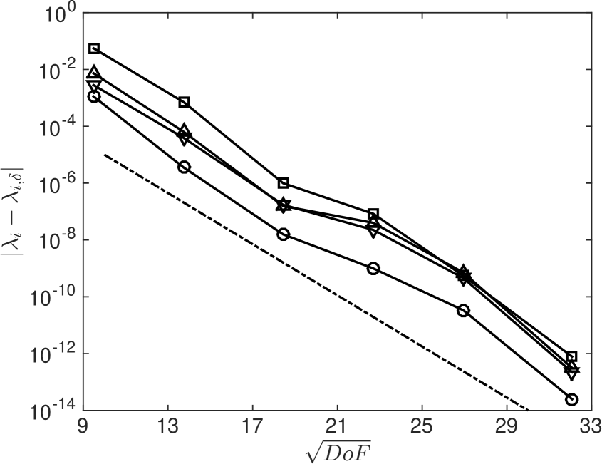
(a). $c=0$.

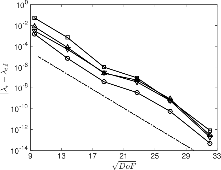
(b). $c=1/2$.

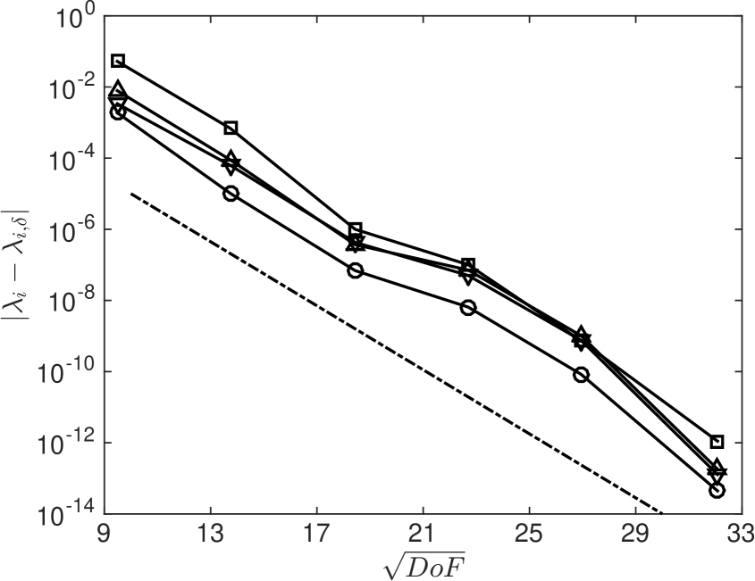
(c). $c=2/3$.

Figure 5.5. MSEM approximation errors $|\lambda_{i}-\lambda_{i,\delta}|$ ($\circ:\lambda_{1}$, $\triangledown:\lambda_{2}$, $\vartriangle:\lambda_{3}$ and $\square:\lambda_{4}$) versus $\sqrt{DoF}$ on the L-shape domain $[-1,1]^{2}\setminus([0,1]\times[-1,0])$: The dash-dot lines are the exponential $y=10^{-0.45\sqrt{DoF}-0.5}$.

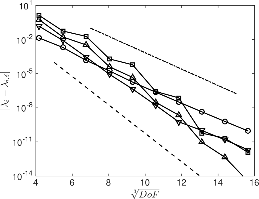
(a). $c=0$.

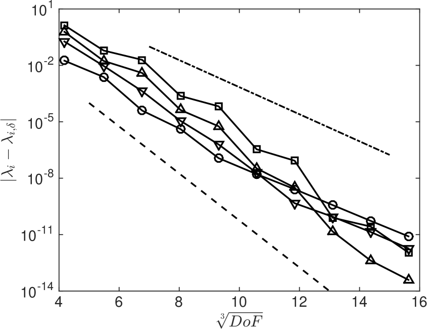
(b). $c=1/2$.

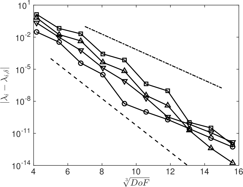
(c). $c=2/3$.

Figure 5.6. GFEM approximation errors $|\lambda_{i}-\lambda_{i,\delta}|$ ($\circ:\lambda_{1}$, $\triangledown:\lambda_{2}$, $\vartriangle:\lambda_{3}$ and $\square:\lambda_{4}$) versus $\sqrt[3]{DoF}$ on the L-shape domain $[-1,1]^{2}\setminus([0,1]\times[-1,0])$. The dashed lines are the exponential $y=10^{-1.25\sqrt[3]{DoF}+2}$, the dash-dot lines are the exponential $y=10^{-0.72\sqrt[3]{DoF}+3.32}$.

Example 3

At last, let us consider the numerical verification of two isospectral geometries, which possess the same Laplacian eigenvalues [5, 22, 11], see Figure 5.7. To carry out the MSEM experiments, we first partition both geometries with four sectors $\Omega_{i}$, $1\leq i\leq 4$, with the radius $R=1/3$, which are located at the vertices of the four reentrant/obtuse corners, respectively. Then $\Omega_{5}:=\Omega\setminus(\cup_{i=1}^{4}\Omega_{i})$ is further decomposed into 10 right triangles (of size $\sqrt{2}$) and 18 curvilinear quadrilaterals, on which the standard $C^{0}$-conforming spectral elements are recommended.

(a)

(b)

Figure 5.7. A pair of isospectral geometries and their nonconforming meshes for MSEM.

We now tabulate the first 25 computed eigenvalues in Table 5.4 with $13$ decimal digits by MSEM with the total degrees of freedom $4457$. The computed eigenvalues are compared with those in 12 digits by Driscoll [11] (also by Betcke and Trefethen [4, 30]). We note that the excerpted eigenvalues in the last column perfectly match the leftmost 12 rounded digits of the approximate eigenvalues on both the geometry (a) and the geometry (b), and the second and the third columns differ only in the rightmost digit. These partially illustrate the isospectral property of the two geometries together with the effectiveness and efficiency of the MSEM proposed in the current paper.

Table 5.4. The 25 smallest numerical Laplacian eigenvalues on the isospectral geometries (a) and (b), together with those excerpted from [11].

No.	MSEM (a)	MSEM (b)	Driscoll
1	2.5379439997986	2.5379439997986	2.53794399980
2	3.6555097135244	3.6555097135244	3.65550971352
3	5.1755593562245	5.1755593562245	5.17555935622
4	6.5375574437644	6.5375574437644	6.53755744376
5	7.2480778625641	7.2480778625641	7.24807786256
6	9.2092949984032	9.2092949984031	9.20929499840
7	10.5969856913332	10.5969856913331	10.5969856913
8	11.5413953955859	11.5413953955859	11.5413953956
9	12.3370055013616	12.3370055013617	12.3370055014
10	13.0536540557280	13.0536540557280	13.0536540557
11	14.3138624642910	14.3138624642910	14.3138624643
12	15.8713026200093	15.8713026200093	15.8713026200
13	16.9417516879721	16.9417516879721	16.9417516880
14	17.6651184368431	17.6651184368430	17.6651184368
15	18.9810673876525	18.9810673876526	18.9810673877
16	20.8823950432823	20.8823950432823	20.8823950433
17	21.2480051773729	21.2480051773729	21.2480051774
18	22.2328517929733	22.2328517929735	22.2328517930
19	23.7112974848240	23.7112974848240	23.7112974848
20	24.4792340692739	24.4792340692739	24.4792340693
21	24.6740110027234	24.6740110027235	24.6740110027
22	26.0802400996599	26.0802400996599	26.0802400997
23	27.3040189211259	27.3040189211260	27.3040189211
24	28.1751285814531	28.1751285814533	28.1751285815
25	29.5697729132392	29.5697729132393	29.5697729132

Conclusion Remarks. In this work, we present a novel and effective way to handle operator singularity of the inverse square potential as well as the domain corner singularities. Although we do not provide a full convergence analysis, numerical evidences indicate that our new methods are superior to existing methods including the $hp$ finite element method using geometric meshes which is known for the best convergence rate with the presence of corner singularities. Therefore, our approach can serve as a better alternative to solve such kind of problems with singularity.

Appendix A The proof of Lemma 3.1 and Lemma 3.2

Let $\nabla_{0}$ be the spherical gradient, which is the spherical part of $\nabla$ and involves only derivatives in $\xi$, i.e.,

$$\nabla_{0}=r(\nabla-\xi\partial_{r}),\qquad x=r\xi,\,\xi\in\mathbb{S}^{d-1}.$$

As a result, $\xi\cdot\nabla_{0}=0$ and

(A.1) $$(\nabla u,\nabla v)_{\Omega}=\big{(}\nabla_{0}u,\nabla_{0}v)_{r^{-2},\Omega}+\big{(}\partial_{r}u,\partial_{r}v)_{\Omega},\quad u,v\in H^{1}(\Omega).$$

Moreover, it holds that ([10, p. 16 and p.  26])

(A.2) $$\Delta_{0}=\nabla_{0}\cdot\nabla_{0},$$

(A.3) $$(\nabla_{0}u,\nabla_{0}v)_{\mathbb{S}^{d-1}}=-(\Delta_{0}u,v)_{\mathbb{S}^{d-1}},\qquad u\in H^{2}(\mathbb{S}^{d-1}),\,v\in H^{1}(\mathbb{S}^{d-1}).$$

We next prove that for any $u,v\in H^{1}(0,1)$,

(A.4) $$\begin{split}\int_{0}^{1}\partial_{r}\big{(}&r^{d/2-1-\beta}u\big{)}\partial_{r}\big{(}r^{d/2-1-\beta}v\big{)}r^{2\beta+1}dr=\int^{1}_{0}\Big{[}r^{2}\partial_{r}u\partial_{r}v+(\beta^{2}-(d/2-1)^{2})uv\Big{]}r^{d-3}dr\\ &+(d/2-1-\beta)[u(1)v(1)-\delta_{d,2}u(0)v(0)].\end{split}$$

Actually, a technical reduction leads to

$$\int_{0}^{1} \partial_{r}\big{[}r^{d/2-1-\beta}u\big{]}\partial_{r}\big{[}r^{d/2-1-\beta}v\big{]}r^{2\beta+1}dr$$

$$= \int_{0}^{1}\Big{[}r^{d-1}\partial_{r}u\partial_{r}u+r^{d-3}(d/2-1-\beta)^{2}uv+(d/2-1-\beta)r^{d-2}\partial_{r}(uv)\Big{]}dr$$

$$= \int_{0}^{1}\Big{[}r^{d-1}\partial_{r}u\partial_{r}u+r^{d-3}(d/2-1-\beta)^{2}uv-(d-2)(d/2-1-\beta)r^{d-3}uv\Big{]}dr$$

$$+(d/2-1-\beta)[u(1)v(1)-0^{d-2}u(0)v(0)]$$

$$= \int^{1}_{0}\Big{[}r^{d-1}\partial_{r}u\partial_{r}v+\big{(}\beta^{2}-(d/2-1)^{2})\big{)}r^{d-3}uv\Big{]}dr+(d/2-1-\beta)[u(1)v(1)-\delta_{d,2}u(0)v(0)],$$

where the second equality sign was derived by integration by part.

We now concentrate on the proofs of Lemma 3.1 and 3.2 in the main body of this paper.

Proof of Lemma 3.1.

We first note that

$$\int_{\mathbb{B}^{d}}u(x)dx=\int_{0}^{1}r^{d-1}dr\int_{\mathbb{S}^{d-1}}u(r\xi)d\sigma(\xi).$$

Then, by (A.1), (A.3) and (2.2), we obtain that

$$\big{(}\nabla Q_{k,\ell}^{n},\nabla Q_{j,\iota}^{m}\big{)}_{\mathbb{B}^{d}}+c^{2}\big{(}Q_{k,\ell}^{n},Q_{j,\iota}^{m}\big{)}_{r^{-2},{\mathbb{B}^{d}}}$$

$$= \,\big{(}\partial_{r}Q_{k,\ell}^{n},\partial_{r}Q_{j,\iota}^{m}\big{)}_{\mathbb{B}^{d}}+\big{(}\nabla_{0}Q_{k,\ell}^{n},\nabla_{0}Q_{j,\iota}^{m}\big{)}_{r^{-2},\mathbb{B}^{d}}+c^{2}\big{(}Q_{k,\ell}^{n},Q_{j,\iota}^{m}\big{)}_{r^{-2},{\mathbb{B}^{d}}}$$

$$= \,\big{(}\partial_{r}Q_{k,\ell}^{n},\partial_{r}Q_{j,\iota}^{m}\big{)}_{\mathbb{B}^{d}}-\big{(}\Delta_{0}Q_{k,\ell}^{n},Q_{j,\iota}^{m}\big{)}_{r^{-2},\mathbb{B}^{d}}+c^{2}\big{(}Q_{k,\ell}^{n},Q_{j,\iota}^{m}\big{)}_{r^{-2},{\mathbb{B}^{d}}}$$

$$= \,\big{(}\partial_{r}Q_{k,\ell}^{n},\partial_{r}Q_{j,\iota}^{m}\big{)}_{\mathbb{B}^{d}}+\big{(}c^{2}+n(n+d-2)\big{)}\big{(}Q_{k,\ell}^{n},Q_{j,\iota}^{m}\big{)}_{r^{-2},{\mathbb{B}^{d}}}.$$

In the sequel, we temporarily set $q_{k,n}(r)=\frac{2k+2\beta_{n}}{k+2\beta_{n}}J^{-1,2\beta_{n}}_{k}(2r-1)r^{\beta_{n}+1-d/2}$ and get further from (A.4), (2.6) , (2.5) and (2.4) that

(A.5) $$\begin{split}\big{(}\nabla&Q_{k,\ell}^{n},\nabla Q_{j,\iota}^{m}\big{)}_{\mathbb{B}^{d}}+c^{2}\big{(}Q_{k,\ell}^{n},Q_{j,\iota}^{m}\big{)}_{r^{-2},{\mathbb{B}^{d}}}\\ =&\,\int_{\SS^{d-1}}Y^{n}_{\ell}(\xi)Y^{m}_{\iota}(\xi)d\sigma(\xi)\int_{0}^{1}\Big{[}r^{d-1}\partial_{r}q_{k,n}\partial_{r}q_{j,n}+\big{(}c^{2}+n(n+d-2)\big{)}r^{d-3}q_{k,n}q_{j,n}\Big{]}dr\\ =&\,\omega_{d}\delta_{m,n}\delta_{\ell,\iota}\int_{0}^{1}\partial_{r}\big{[}r^{d/2-1-\beta_{n}}q_{k,n}\big{]}\partial_{r}\big{[}r^{d/2-1-\beta_{n}}q_{j,n}\big{]}r^{2\beta_{n}+1}dr\\ &\,+\,\omega_{d}\delta_{m,n}\delta_{\ell,\iota}(\beta_{n}+1-d/2)[q_{k,n}(1)q_{j,n}(1)-\delta_{d,2}q_{k,n}(0)q_{j,n}(0)]\\ =&\,\omega_{d}\delta_{m,n}\delta_{\ell,\iota}\frac{(2k+2\beta_{n})(2j+2\beta_{n})}{(k+2\beta_{n})(j+2\beta_{n})}\int_{0}^{1}\partial_{r}J^{-1,2\beta_{n}}_{k}(2r-1)\partial_{r}J^{-1,2\beta_{n}}_{j}(2r-1)r^{2\beta_{n}+1}dr\\ &\,+\,\omega_{d}\delta_{m,n}\delta_{\ell,\iota}(\beta_{n}+1-d/2)\frac{(2k+2\beta_{n})(2j+2\beta_{n})}{(k+2\beta_{n})(j+2\beta_{n})}[\delta_{k,0}\delta_{j,k}-\delta_{\beta_{n}+1-d/2,0}\delta_{d,2}]\\ =&\,\omega_{d}\delta_{m,n}\delta_{\ell,\iota}(2k+2\beta_{n})(2j+2\beta_{n})\int_{0}^{1}J^{0,2\beta_{n}+1}_{k-1}(2r-1)J^{0,2\beta_{n}+1}_{j-1}(2r-1)r^{2\beta_{n}+1}dr\\ &\,+\,\omega_{d}\delta_{m,n}\delta_{\ell,\iota}(\beta_{n}+1-d/2)\delta_{k,0}\delta_{j,k}\\ =&\,\omega_{d}\delta_{m,n}\delta_{\ell,\iota}\delta_{k,j}\left[(2k+2\beta_{n})(1-\delta_{k,0})+(\beta_{n}-d/2+1)\delta_{k,0}\right],\end{split}$$

which gives (3.1).

Next, it is easy to see that

(A.6) $$\begin{split}(Q_{k,\ell}^{n},&Q_{j,\iota}^{m})_{\mathbb{B}^{d}}=\,\int_{\mathbb{S}^{d-1}}Y_{\ell}^{n}(\xi)Y_{\ell}^{n}(\xi)d\sigma(\xi)\\ &\times\frac{(2k+2\beta_{n})(2j+2\beta_{m})}{(k+2\beta_{n})(j+2\beta_{m})}\int_{0}^{1}J^{-1,2\beta_{n}}_{k}(2r-1)J^{-1,2\beta_{m}}_{j}(2r-1)r^{\beta_{n}+\beta_{m}+1}dr\,\\ =&\,\omega_{d}\delta_{n,m}\delta_{k,j}\frac{(2k+2\beta_{n})(2j+2\beta_{m})}{(k+2\beta_{n})(j+2\beta_{m})}\int_{0}^{1}J^{-1,2\beta_{n}}_{k}(2r-1)J^{-1,2\beta_{m}}_{j}(2r-1)r^{2\beta_{n}+1}dr.\end{split}$$

To proceed the proof of (3.2), we shall resort to the following identity on generalized Jacobi polynomials,

(A.7) $$J^{\alpha,\beta}_{k}(\zeta)=\frac{k+\alpha+\beta+1}{2k+\alpha+\beta+1}J^{\alpha+1,\beta}_{k}(\zeta)-\frac{k+\beta}{2k+\alpha+\beta+1}J^{\alpha+1,\beta}_{k-1}(\zeta),$$

which is stemmed from [1, p. 304] by extension. Using (A.7) twice together with (2.8) yields

$$\begin{split}&J^{\alpha,\beta}_{k}(\zeta)=\frac{(k+\alpha+\beta+1)(k+\alpha+\beta+2)}{(2k+\alpha+\beta+1)(2k+\alpha+\beta+2)}J^{\alpha+1,\beta+1}_{k}(\zeta)\\ &\quad+\frac{(\alpha-\beta)(k+\alpha+\beta+1)}{(2k+\alpha+\beta)(2k+\alpha+\beta+2)}J^{\alpha+1,\beta+1}_{k-1}(\zeta)-\frac{(k+\alpha)(k+\beta)}{(2k+\alpha+\beta)(2k+\alpha+\beta+1)}J^{\alpha+1,\beta+1}_{k-2}(\zeta).\end{split}$$

In particular,

(A.8) $$\frac{2k+\beta}{k+\beta}J_{k}^{-1,\beta}=\frac{k+\beta+1}{2k+\beta+1}J_{k}^{0,\beta+1}-\frac{(1+\beta)(2k+\beta)}{(2k+\beta-1)(2k+\beta+1)}J_{k-1}^{0,\beta+1}-\frac{k-1}{2k+\beta-1}J_{k-2}^{0,\beta+1}.$$

Then a combination of (A.6), (A.8) and (2.4) immediately yields (3.2). This completes the proof of Lemma 3.2.  

Proof of Lemma 3.2.

Let us temporarily set $p_{k,n}(r)=\frac{2k+\beta_{n}}{k+\beta_{n}}J^{-1,\beta_{n}}_{k}(2r^{2}-1)r^{\beta_{n}+1-d/2}$. Then a similar reduction as in (A.5) yields

$$\big{(}\nabla P_{k,\ell}^{n},\nabla P_{j,\iota}^{m}\big{)}_{\mathbb{B}^{d}}+c^{2}\big{(}P_{k,\ell}^{n},P_{j,\iota}^{m}\big{)}_{r^{-2},{\mathbb{B}^{d}}}$$

$$= \,\omega_{d}\delta_{m,n}\delta_{\ell,\iota}\int_{0}^{1}\partial_{r}\big{[}r^{d/2-1-\beta_{n}}p_{k,n}\big{]}\partial_{r}\big{[}r^{d/2-1-\beta_{n}}p_{j,n}\big{]}r^{2\beta_{n}+1}dr$$

$$\,+\,\omega_{d}\delta_{m,n}\delta_{\ell,\iota}(\beta+1-d/2)[p_{k,n}(1)p_{j,n}(1)-\delta_{d,2}p_{k,n}(0)p_{j,n}(0)]$$

$$= \,\omega_{d}\delta_{m,n}\delta_{\ell,\iota}\frac{(2k+\beta_{n})(2j+\beta_{n})}{(k+\beta_{n})(j+\beta_{n})}\int_{0}^{1}\partial_{r}J^{-1,\beta_{n}}_{k}(2r^{2}-1)\partial_{r}J^{-1,\beta_{n}}_{j}(2r^{2}-1)r^{2\beta_{n}+1}dr$$

$$\,+\,\omega_{d}\delta_{m,n}\delta_{\ell,\iota}(\beta_{n}+1-d/2)\frac{(2k+\beta_{n})(2j+\beta_{n})}{(k+\beta_{n})(j+\beta_{n})}[\delta_{k,0}\delta_{j,k}-\delta_{\beta_{n}+1-d/2,0}\delta_{d,2}]$$

$$= \,\omega_{d}\delta_{m,n}\delta_{\ell,\iota}2(2k+\beta_{n})(2j+\beta_{n})\int_{0}^{1}J^{0,\beta_{n}+1}_{k-1}(2r^{2}-1)J^{0,\beta_{n}+1}_{j-1}(2r^{2}-1)r^{2\beta_{n}+2}dr^{2}$$

$$\,+\,\omega_{d}\delta_{m,n}\delta_{\ell,\iota}(\beta_{n}+1-d/2)\delta_{k,0}\delta_{j,k}$$

$$= \,\omega_{d}\delta_{m,n}\delta_{\ell,\iota}\delta_{k,j}\left[2(2k+\beta_{n})(1-\delta_{k,0})+(\beta_{n}-d/2+1)\delta_{k,0}\right],$$

which gives (3.5).

Further, we note that

$$\begin{split}(P_{k,\ell}^{n},P_{j,\iota}^{m})_{\mathbb{B}^{d}}=&\,\omega_{d}\delta_{n,m}\delta_{k,j}\frac{(2k+\beta_{n})(2j+\beta_{m})}{(k+\beta_{n})(j+\beta_{m})}\int_{0}^{1}J^{-1,\beta_{n}}_{k}(2r^{2}-1)J^{-1,\beta_{m}}_{j}(2r^{2}-1)r^{2\beta_{n}+1}dr.\end{split}$$

Then (3.6) is an immediate consequence of (A.7) and (2.4). This proof of Lemma 3.2 is now completed.

References

- [1] G. E. Andrews, R. Askey, and R. Ranjan, Special Functions, Cambridge University Press, Cambridge, 1999.
- [2] I. M. Babuška and B. Guo, Approximation properties of the - version of finite element method, Comput. Method, Appl. Mech. Engrg., 133 (1996), pp. 319–346.
- [3] C. Bernardi, Y. Maday, and F. Rapetti, Basics and some applications of the mortar element method, GAMM-Mitt., 28 (2005), pp. 97–123.
- [4] T. Betcke and L. N. Trefethen, Reviving the method of particular solutions, SIAM Rev., 47 (2005), pp. 469–491.
- [5] P. Buser, J. Conway, P. Doyle, and K.-D. Semmler, Some planar isospectral domains, in Internat. Math. Res. Notices, 1994, pp. 391–400.
- [6] C. Bǎcutǎ, V. Nistor, and L. T. Zikatanov, Improving the rate of convergence of “high order finite elements” on polygons and domains with cusps, Numerische Mathematik, 100 (2005), pp. 165–184.
- [7] C. Canuto, M. Y. Hussaini, A. Quarteroni, and T. A. Zang, Spectral Methods: Evolution to Complex Geometries and Applications to Fluid Dynamics, Springer, 2007.
- [8] D. Cao and P. Han, Solutions to critical elliptic equations with multi-singular inverse square potentials, J. Differential Equations, 224 (2006), pp. 332–372.
- [9] K. M. Case, Singular potentials, Physical Rev., 80 (1950), pp. 797–806.
- [10] F. Dai and Y. Xu, Approximation Theory and Harmonic Analysis on Spherical and Balls, Springer, New York, 2013.
- [11] T. A. Driscoll, Eigenmodes of isospectral drums, SIAM Rev., 39 (1997), pp. 1–17.
- [12] C. F. Dunkl and Y. Xu, Orthogonal Polynomials of Several Variables, vol. 155, Cambridge University Press, 2014.
- [13] V. Felli, E. M. Marchini, and S. Terracini, On Schrödinger operators with multipolar inverse-square potentials, Journal of Functional Analysis, 250 (2007), pp. 265–316.
- [14] V. Felli and S. Terracini, Elliptic equations with multi-singular inverse-square potentials and critical nonlinearity, Comm. Partial Differential Equations., 31 (2006), pp. 469–495.
- [15] W. M. Frank, D. J. Land, and S. R. M., Singular potentials, Rev. Modern Phys., 43 (1971), pp. 36–98.
- [16] P. Grisvard, Elliptic Problems in Nonsmooth Domains, vol. 24, Pitman (Advanced Publishing Program), 1985.
- [17] W. Gui and I. Babuška, The , and versions of the finite element method in 1 dimension. Part I. The error analysis of the -version, Numer. Math., 43 (1986), pp. 577–612.
- [18] , The , and versions of the finite element method in 1 dimension. Part II. The error analysis of the h and h-p versions, Numer. Math., 43 (1986), pp. 613–658.
- [19] , The , and versions of the finite element method in 1 dimension. Part III. The adaptive h-p version, Numer. Math., 49 (1986), pp. 659–684.
- [20] B. Guo and W. Sun, The optimal convergence of the - version of the finite element method with quasi-uniform meshes, SIAM Journal on Numerical Analysis, 45 (2007), pp. 698–730.
- [21] B.-Y. Guo, J. Shen, and L.-L. Wang, Optimal spectral-Galerkin methods using generalized Jacobi polynomials, Journal of Scientific Computing, 27 (2006), pp. 305–322.
- [22] M. Kac, Can one hear the shape of a drum?, Amer. Math. Monthly, 73 (1996), pp. 1–23.
- [23] H. Kalf, U. W. Schmincke, J. Walter, and R. Wüst, On the spectral theory of Schrödinger and Dirac operators with strongly singular potentials, in Spectral Theory and Differential Equations, vol. 448 of Lect. Notes in Math., Springer, Berlin, 1975, pp. 182–226.
- [24] H. Li and J. S. Ovall, A posteriori estimation of hierarchical type for the Schrödinger operator with the inverse square potential on graded meshes, Numerische Mathematik, 128 (2014), pp. 707–740.
- [25] , A posteriori eigenvalue error estimation for the Schrödinger operator with the inverse square potential, Discrete and Continuous Dynamical Systems – Series B, 20 (2015), pp. 1377–1391.
- [26] H. Li and J. Shen, Optimal error estimates in Jacobi-weighted Sobolev spaces for polynomial approximations on the triangle, Mathematics of Computation, 79 (2010), pp. 1621–1646.
- [27] H. Li and Y. Xu, Spectral approximation on the unit ball, SIAM Journal on Numerical Analysis, 52 (2014), pp. 2647–2675.
- [28] G. W. Reddien, Finite-difference approximations to singular Sturm-Liouville eigenvalue problems, Math. Comp., 30 (1976), pp. 278–282.
- [29] J. Shen, Efficient spectral-Galerkin method III: Polar and cylindrical geometries, SIAM J. Sci. Comput., 18 (1997), pp. 1583–1604.
- [30] L. N. Trefethen and T. Betcke, Computed eigenmodes of planar regions, Recent Advances In Differential Equations And Mathematical Physics,Contemporary Mathematics, 412 (2006), pp. 297–314.
- [31] H. Weyl, Ueber die asymptotische verteilung der eigenwerte, Nachrichten von der Gesellschaft der Wissenschaften zu Göttingen, Mathematisch-Physikalische Klasse, 1911 (1911), pp. 110–117.