An Empirical Approach to Cosmological Galaxy Survey Simulation: Application to SPHEREx Low Resolution Spectroscopy

Abstract

Highly accurate models of the galaxy population over cosmological volumes are necessary in order to predict the performance of upcoming cosmological missions. We present a data-driven model of the galaxy population constrained by deep 0.1–8 $\rm\mu m$ imaging and spectroscopic data in the COSMOS survey, with the immediate goal of simulating the spectroscopic redshift performance of the proposed SPHEREx mission. SPHEREx will obtain over the full-sky $R\sim 41$ spectrophotometry at moderate spatial resolution ($\sim 6$″) over the wavelength range 0.75–4.18 $\rm\mu m$ and $R\sim 135$ over the wavelength range 4.18–5 $\rm\mu m$ . We show that our simulation accurately reproduces a range of known galaxy properties, encapsulating the full complexity of the galaxy population and enables realistic, full end-to-end simulations to predict mission performance. Finally, we discuss potential applications of the simulation framework to future cosmology missions and give a description of released data products.

1. Introduction

Low-resolution ($R\sim 20$–100) spectroscopy and photometric redshifts (photo-z’s) based on $R\lesssim 10$ broad-band photometry are now widely accepted as powerful tools for galaxy evolution studies and precision cosmology. Current surveys such as CANDELS (Koekemoer et al., 2011), COSMOS (Scoville et al., 2007), ALHAMBRA (Moles et al., 2008), and PRIMUS (Coil et al., 2011; Cool et al., 2013) have successfully used $R\sim 5$–100 spectrophotometry to estimate redshifts for a wide variety of sources with great success. Furthermore, upcoming “Stage IV” dark energy experiments such as LSST, Euclid, and WFIRST will rely critically on photometric redshifts for weak lensing cosmology.

A key shortcoming in galaxy simulations aimed at informing cosmology missions has been that the photo-z performance predicted by such simulations is typically overestimated compared to actual performance. This is largely due the inherent complexity of the galaxy population—which is rarely captured in simulations—combined with the myriad systematic effects that increase the noise in spectrophotometry and are difficult to model without full end-to-end simulations. Cosmological simulations based on the actual, measured galaxy population that account for all sources of measurement errors would therefore represent a major improvement in terms of capturing the true complexity that cosmological surveys would encounter.

In this paper, we present a simulation framework aimed at capturing the full complexity of the galaxy population using deep, 30-band data in the well-studied COSMOS field (Scoville et al., 2007; Laigle et al., 2016). This field includes very deep 0.1–8 $\rm\mu m$ data with spectral resolution of $R\sim 5$–20 as well as X-ray and longer wavelength data. In addition, high-quality redshifts are available to $\sim$25,000 galaxies, and a new survey is underway to obtain spectra fully representative of the galaxy population (Masters et al. in prep). Furthermore, photometric redshifts accurate to $dz/(1+z)<0.01$ are available for most galaxies. With these data, the spectral energy distributions (SEDs) of the galaxies are very well constrained, so the fluxes in unknown bands in the 0.1–8 $\rm\mu m$ range can be estimated to high-precision via interpolation, rather than extrapolation. The resulting simulation accurately reproduces narrow and intermediate band photometry not used to generate the model. A wide range of galaxy population properties, such as the stellar masses, star formation rates, and emission line characteristics of galaxies are thereby accurately reproduced.

In addition to the SEDs, high-resolution Hubble Space Telescope (HST) imaging and galaxy physical property (star formation rate, stellar mass) measurements are available in the COSMOS field (Laigle et al., 2016). The galaxies are also tied to their dark matter halo properties using a combination of weak lensing, clustering, and abundance matching (Leauthaud et al. 2012). With this information, it is straightforward to propagate the interpolative photometry model to cosmological constraints.

We apply this simulation framework to an end-to-end simulation of the proposed SPHEREx mission, which will obtain $R\sim 40$ spectrophotometry over the wavelength range 0.75–4.18 $\rm\mu m$ and $R\sim 135$ over the wavelength range 4.18–5 $\rm\mu m$ for the full sky at moderate (6.2″) spatial resolution (Doré et al., 2014). The simulation includes source confusion, selection effects, systematic calibration errors, and photometric extraction errors. Using this end-to-end simulation, we realistically constrain the expected redshift performance of the proposed SPHEREx mission, and the resulting cosmological constraints.

The outline of this paper is as follows. In §2, we outline the simulation philosophy. In §3, we give an overview of the proposed SPHEREx mission. In §4, we present the methodology used to generate realistic mock SPHEREx data based on the COSMOS survey. In §5 we describe the simulation pipeline in detail. In §6, we conclude with a discussion of how similar simulations may benefit a number of upcoming cosmology missions, such as LSST (LSST Science Collaboration et al., 2009), Euclid (Laureijs et al., 2011), and WFIRST (Spergel et al., 2015). We also discuss potential applications to predicting the performance of spectroscopic surveys such as PFS Takada et al. (2014) and DESI (Levi et al., 2013).

2. Simulation Philosophy

The key idea behind the SPHEREx simulation is to stay as close to reality as possible by using the well-constrained galaxy photometry in the COSMOS field to generate realistic simulated photometry. Rather than try to simulate the dark matter structure of the universe and paint on galaxies, we let the observed universe in the COSMOS field drive the simulated observations. In this way, we ensure that the simulated data captures the complexity of the real world.

Galaxies in the COSMOS field have deep, 30-band photometric data and accurate photometric redshifts, in addition to other measured quantities. To predict the SPHEREx observations, intrinsic spectral energy distributions (SEDs) of the galaxies must be assumed. We use the state-of-the-art galaxy spectral templates from Brown et al. (2014), an empirically-based set of SEDs representing a wide range of galaxy types, to assign a realistic SED to each galaxy in COSMOS, including emission lines. This is accomplised by fitting the templates to the observed COSMOS photometry, which is highly constraining over the relevant wavelength range. This data-driven SED then feeds forward into the simulated SPHEREx photometry. Critically, the effects of blended photometry and the realistic distribution of galaxy properties in the universe are automatically modeled with this approach.

3. SPHEREx Overview

SPHEREx (Spectro-Photometer for the History of the Universe, Epoch of Reionization, and Ices Explorer) is a proposed all-sky survey satellite designed to address all three science goals in NASA’s Astrophysics Division: probe the origin and destiny of our Universe; explore whether planets around other stars could harbor life; and explore the origin and evolution of galaxies. SPHEREx will probe the origin of the Universe by constraining the physics of inflation, the superluminal expansion of the Universe that took place some $10^{-32}$ s after the Big Bang (Doré et al., 2014). SPHEREx will study the imprint of inflation in the three-dimensional large-scale distribution of matter by measuring galaxy redshifts over a large cosmological volume at low redshifts, complementing high-redshift surveys optimized to constrain dark energy. SPHEREx will also investigate the origin of water and biogenic molecules in all phases of planetary system formation—from molecular clouds to young stellar systems with protoplanetary disks—by measuring absorption spectra to determine the abundance and composition of ices toward $>2\times 10^{4}$ Galactic targets. SPHEREx will chart the origin and history of galaxy formation through a deep survey mapping large-scale structure. This technique measures the total light produced by all galaxy populations, complementing studies based on deep galaxy counts, to trace the history of galactic light production from the present day to the first galaxies that ended the cosmic dark ages. SPHEREx will be the first all-sky near-infrared spectral survey, creating a legacy archive of spectra ($0.75\leq\lambda\leq 4.18$ $\rm\mu m$ with $\lambda/\Delta\lambda=41.4$, and a narrower filter width $\lambda/\Delta\lambda=135$ in the range $\lambda=4.18$–$5$ $\rm\mu m$) with the high sensitivity obtained using a cooled telescope 4with large spectral mapping speed.

The SPHEREx Mission will implement a simple, robust design that maximizes spectral throughput and efficiency. The instrument is based on a 20 cm all-aluminum telescope with a wide $3.5^{\circ}\times 7^{\circ}$ field of view, imaged onto four $\rm 2k\times 2k$ HgCdTe detector arrays arranged in pairs, separated by a dichroic. Spectra are produced by four linear-variable filters (LVFs). The spectrum of each source is obtained by moving the telescope across the dispersion direction of the filter in a series of discrete steps—a method demonstrated by LEISA on New Horizons (Elliott et al., 2016). SPHEREx has no moving parts except for one-time deployments of the sun shields and aperture cover. It will observe from a sun-synchronous terminator low-earth orbit, scanning repeatedly to cover the entire sky in a manner similar to IRAS (Neugebauer et al., 1984), COBE (Smoot et al., 1992) and WISE (Wright et al., 2010). During its two-year nominal mission, SPHEREx produces four complete all-sky spectral maps for constraining the physics of inflation. The orbit naturally covers two deep, highly redundant regions at the celestial poles, which we use to make a deep map, ideal for studying galaxy evolution and monitor instrument performances.

4. Simulating the SPHEREx Data using the COSMOS Survey

To accurately assess the ability of SPHEREx to recover redshifts, the simulation must include the full observed diversity in both the broad SEDs and emission line features of galaxies. Furthermore, blends of objects and artifacts that produce spectra with biased redshifts must also be simulated to accurately represent the redshift ambiguity in the data.

To ensure this level of representativeness, we use data from the Cosmic Evolution Survey (COSMOS, Scoville et al., 2007; Capak et al., 2007). COSMOS is a multi-waveband survey of a 2-deg² patch of equatorial sky with observations from the X-ray to the radio. COSMOS is built around deep HST-ACS imaging in $i$-band, with imaging in a number of ground-based telescopes and other major space-based observatories providing broad and intermediate band imaging over 0.1–8 $\rm\mu m$ at a resolution of $R=5$–20. COSMOS therefore covers the SPHEREx wavelength range at similar (though slightly lower) spectral resolution, but is more than 100 times as sensitive and has more than five times the spatial resolution. Furthermore, a fully representative spectroscopic data set is available at the SPHEREx flux limits in COSMOS.

To interpolate to the higher spectral resolution of SPHEREx, we use the observed Galaxy templates from Brown et al. (2014), AGN (Salvato et al., 2011), and stars Chabrier et al. (2000), which span the range of expected object properties and include all of the key features we will observe with SPHEREx. We note that this pipeline is an extension of the pipeline used to produce official forecasts for the Euclid consortium, the WFIRST Science Definition Team, as well as the Hyper Suprime-Cam (HSC) Subaru survey.

5. Simulation Pipeline Overview

There are four main steps to the SPHEREx simulation pipeline: 1) Create an input galaxy catalog, based on real data from the multi-wavelength COSMOS survey. 2) Generate simulated SPHEREx images at each wavelength step of the SPHEREx LVFs. 3) Optimally extract the photometry from the simulated SPHEREx images. 4) Derive the photometric redshifts for all detected objects. In this section, we describe these steps in detail.

5.1. Galaxy redshifts and spectral energy distributions from COSMOS

We use the COSMOS 2-deg² Laigle et al. (2016) COSMOS multi-band catalog as the starting point of our simulation. The catalog includes some of the deepest available spectro-photometry from 0.1 $\rm\mu m$ to 8 $\rm\mu m$. It was selected at 0.9–2.5 $\rm\mu m$ (similar to SPHEREx), using a combination of Subaru Suprime-Cam and UltraVISTA DR2 imaging (McCracken et al., 2013). The catalog is 95% complete to ${\rm z}^{\prime}<25.5$ (0.9 $\rm\mu m$) and ${\rm Ks}<24.5$ (2.5 $\rm\mu m$) AB magnitudes and includes data of equivalent depth from 0.1–8 $\rm\mu m$. The Laigle et al. (2016) data have been shown to produce photometric redshifts precise to $\sigma(z)/(1+z)<0.02$ with a very low outlier fraction at SPHEREx depths. Furthermore, the accuracy, precision, and other properties of the photometric redshifts has been verified with a representative spectroscopic sample at SPHEREx depths (Masters et al., 2015). As a result, for all objects in the COSMOS field detectable by SPHEREx, the observed SEDs and redshifts are known. The observational data in COSMOS reach two orders of magnitude fainter in flux than will be detectable by SPHEREx, so the effects of confusion and blending can be accurately modeled in our simulations.

The spectroscopic catalog produced from this photometry includes a classifier for galaxies, AGN, and stars based on the full photometric data set along with X-ray and radio data to select AGN. We acknowledge the fact that there are more robust classifiers for AGN and better redshift determinations than Laigle et al. (2016) (for instance, Salvato et al., 2011). However, for the purposes of simulating the photometry and the performance of spectroscopic redshift or photo-z, the exact classification and redshift distribution has little effect. Specifically, the main impact of AGN on photo-z performance is the template confusion and the method outlined in this paper accurately reproduces that effect.

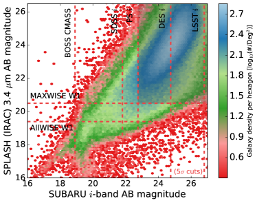
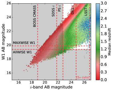
Figure 1.— Magnitude-magnitude plots of the COSMOS data. In both panels, the vertical and horizontal lines indicate 5 $\sigma$ depths for various relevant surveys / instruments . All the objects in this plot are included in our simulations. The gray shaded region identify objects that contribute to the confusion background in the simulations but are not selected to be in the SPHEREx catalog as being not bright enough in WISE or PanSTARRS. Left panel: The actual COSMOS catalog in the IRAC channel 1 $i$-band color space from the Spitzer survey and the Subaru telescope (by design, IRAC channel 1 is a good proxy for the WISE W1 band). Photometric artefacts appearing around $i$-band M${}_{AB}\sim$ 19 are not corrected. The color of the hexagonal bins encodes the angular density of detected objects. Right panel: Simulated data from the based simulation in the WISE W1–$i$ color space. The color of the hexagonal bins encodes the median redshift within a bin.

Figure 1 demonstrates how well the simulation reproduces the scatter in the COSMOS data. The SPHEREx spectroscopic catalog is represented by the non gray shaded area (i.e., the objects detected in Pan-STARRS PS1 $i$-band or WISE W1). It also demonstrates the fact that the simulation is based on a data set that is much deeper than the SPHEREx depth, thus allowing an accurate modeling of confusion and blending.

5.2. Determination of SPHEREx fluxes

Figure 2.— The COSMOS filters used to constrain the Brown et al. templates are shown in black (COSMOS Used), however the GALEX filters at 0.15$\mu$m and 0.25$\mu$m have been omitted for clarity. COSMOS filters not used to constrain the templates whose fluxes were predicted as a verification of the method are shown in red (COSMOS Not Used). The SPHEREx bands on the spacecraft are shown in brown (SPHEREx Bands), while the external data from PS1 and WISE are shown in blue (SPHEREx external).

SPHEREx will reach $R\sim 41.5$ with continuous coverage from 0.7–4.5 $\rm\mu m$. However, the COSMOS photometry in the 0.7–5 $\rm\mu m$  range is $R\sim 5$–20 and has gaps in the 1–3 $\rm\mu m$  range, due to atmospheric absorption (See Figure 2), so we must interpolate from the COSMOS data to SPHEREx spectral resolution. Despite the fact that some spectral information is missing, SED templates are highly constrained by the COSMOS data, due to its depth, spectral resolution, and spectral coverage. The performance of the simulation is not highly sensitive to the choice of template set because the interpolation between bands is relatively small. The most important aspect of the choice of template library is the diversity of high-resolution ($R>10$) spectral properties between 1–3 $\rm\mu m$, which are not completely constrained by the $R\sim 5$ photometry. For galaxies, we chose the Brown et al. (2014) observed 0.1–100 $\rm\mu m$  templates for the interpolation. These templates were selected to represent the range of colors observed in local galaxies, and are constructed from observed spectra whenever possible and photometry when spectra were unavailable. They include the effects of extinction, complex morphology, and a range of emission line strengths. We augment the library by adding additional extinction to the templates to represent heavily obscured sources. The Calzetti et al. (2000), Prevot et al. (1984), Fitzpatrick & Massa (1986), Seaton (1979), and Allen (1976) laws were used, with additional extinction of up to an $E(B-V)$ of 1.0 added. In addition to the Brown et al. (2014) templates, the Salvato et al. (2011) templates were used to represent known AGN in the COSMOS field. These templates were chosen to represent the range of known AGN from broad line QSO to liners and, like the Brown et al. (2014) templates, are tied to observed spectra and photometry. Finally, for stars the Chabrier et al. (2000) library was used.

We note that several other template sets were considered for the interpolation. These included the Bruzual & Charlot (2003) templates, the Ilbert et al. (2009) templates, and the MAGPHYS (da Cunha et al., 2012) templates. The Bruzual & Charlot (2003) templates were rejected because they included neither dust emission, which dominates the SEDs at $>1$ $\rm\mu m$, nor emission lines, which will be a significant effect at the spectral resolution of SPHEREx. The Ilbert et al. (2009) templates were used in early iterations of these simulations, but were replaced because they were not fully representative of the diversity of emission lines and $>1$ $\rm\mu m$  SEDs observed in galaxies. Finally, the MAGPHYS templates were considered, but were found to be inferior to the Brown et al. (2014) templates because they did not include optical or NIR emission lines and were not as well-constrained by observations.

In order to fit templates to the COSMOS photometry, we first partitioned the catalog, based on the Laigle et al. (2016) classifications, to create separate galaxy, AGN, and stellar catalogs. For each galaxy and AGN SED, we modified the templates in the respective template libraries (Brown et al. templates for galaxies and Savato templates for AGNs) so that the redshifts of the templates matched the estimated redshifts from Laigle et al. (2016). We modified the extinction of each template, as discussed above, and then identified the combination of template, reddening law, and $E(B-V)$ which best fit the photometry (i.e., the combination of parameters which minimized the $\chi^{2}$ discrepancy between the model SED and the measured photometry). In the remainder of this paper, we refer to the combination of template, redshift, reddening law, and $E(B-V)$ as a model SED. For stars, we simply assigned the best-fitting Chabrier et al. (2000) template.

The best-fitting model SED was then used to interpolate from the COSMOS photometry to the SPHEREx bands using the LVF filter profiles, spaced at $R=41.5$ with Nyquist sampling. The Pan-STARRS PS1 (Kaiser et al., 2002; Kaiser, 2004) and ALLWISE band fluxes are also estimated. COSMOS

5.3. SPHEREx image simulation

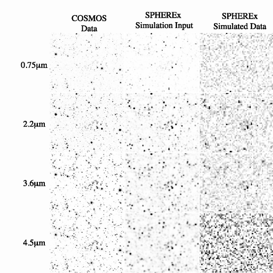
Figure 3.— A comparison of real and simulated images in four bands. Each sub-plot shows the $5^{\prime}\times 5^{\prime}$ region at the center of the COSMOS field. The left panels show real observational data. The center panels show the high-resolution, noiseless simulated images generated by the pipeline, and the right panels show the lower resolution, final images after noise has been added.

To simulate the effects of confusion, calibration, and extraction on the photometry we constructed an end-to-end simulation of the images, photometric extraction, and redshift recovery. We begin with the predicted fluxes in §5.2. These fluxes are then added to a set of simulated images (one image for each SPHEREx band), oversampled by a factor of 8 relative to the SPHEREx detector (i.e., to a grid with pixel scale 6$\farcs$2/8). All sources in the Laigle et al. (2016) catalog are placed in the simulated images, reaching to over 100 times the detection limit of SPHEREx.

These images are then smoothed with a Gaussian of $1.22\lambda/D$ to simulate diffraction, a 1.55″ FWHM Gaussian (4.5 $\rm\mu m$  scaled to the plate scale of the detector) to simulate optical aberration, which dominates over diffraction (by design) for much of the wavelength coverage. A 8.4”″ FWHM Gaussian to simulate pointing error. The image is then binned to the SPHEREx pixel scale. Based on instrument simulations, a random multiplicative error of 0.32% is applied to each pixel to represent the worst case flat fielding error and an additive error of between 2–4 $\rm\mu Jy$ (depending on wavelength) to represent sky background subtraction error. Finally, Gaussian noise is added at the expected RMS background level.

5.4. Source extraction and sample properties

To extract photometry, we use the Pan-STARRSP̃S1 and ALLWISE catalogs for source identification and astrometry. A median background is subtracted from all sources to correct for the mean contribution of undetected/unknown sources. The SPHEREx PSF at the object position is used to perform optimal flux extraction, taking into account the pixel response function of both the primary pixel on which the object falls as well as neighboring pixels. This is done for each SPHEREx band.

For an unresolved source in a survey with a well-known PSF, $P$, the optimal photometric extraction of the total flux, $F$, is obtained by the weighted sum,

$$F=\sum_{ij}w_{ij}D_{ij},$$ (1)

where $D_{ij}$ is the sky-subtracted flux measured in pixel $(i,j)$ and the weight function $w_{ij}$ is

$$w_{ij}=\frac{P_{ij}}{\sum_{ij}P^{2}_{ij}}.$$ (2)

Here $P_{ij}$ is the fraction of the PSF falling in pixel $(i,j)$. In the all-sky survey proposed for SPHEREx  the noise budget is dominated by photon noise from zodiacal light, which is diffuse and nearly uniform across the FOV. To quantify the signal-to-noise of a given detection and how it varies with the relative alignment of the detector grid, it is useful to define the parameter

$$N_{\rm eff}=\sum_{ij}P_{ij}^{-2},$$ (3)

which represents the effective number of pixels spanned by the PSF. As $N_{\rm eff}$ increases, the signal from the source is spread over more pixels and the noise increases by the square root of the number of pixels. Therefore, in optimal photometry, the uncertainty in recovered source flux is related to $N_{\rm eff}$ by

$$\delta F=\delta F(1)\sqrt{N_{\rm eff}}$$ (4)

where $\delta F(1)$ is the uncertainty in flux achieved for a PSF which is a perfect single-pixel square step function.

For SPHEREx, $N_{\rm eff}$ will increase systematically with wavelength, due to the growth of the diffraction limited PSF. Additionally, for a single wavelength, there is a significant spread in $N_{\rm eff}$, caused by the random alignment of sources with the detector grid. If a source falls closer to the corner of a pixel, its flux will spill over to neighboring pixels, while a source landing in the center will deposit most of its energy in a single pixel.

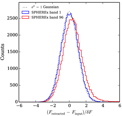
Figure 4.— Histograms showing the relationship between the input fluxes ($F_{\rm input}$) and fluxes extracted from synthetic images ($F_{\rm extracted}$). The dotted black line shows the ideal case, in which the extracted fluxes are perfectly consistent with the input fluxes, after taking the measurement errors ($\delta F$) into account. The blue and red histograms show the shortest and longest wavelength bands of SPHEREx, respectively. Contamination from neighboring objects tends to cause a positive offset in the extracted fluxes. Longer wavelengths are more strongly affected than shorter wavelenths because the PSF increases with wavelength.

With the position of the object known, from Pan-STARRS and ALLWISE, the absolute pointing reconstructed to $<1$″, and the PSF accurately characterized in every image, the values of $P_{ij}$ that go into the weight function for optimal extraction can be computed. To do this, the normalized PSF is resampled onto a fine grid centered at the known position of the object on the detector, and the value of $P_{ij}$ in the nearby pixels is found by summing the portion of $P$ falling within pixel $(i,j)$.

In general, the optimally extracted object fluxes match the input fluxes well—particularly for brighter objects in the input catalog. However, there can be significant contamination, in particular for fainter objects with contaminating objects that fall in the same or neighboring SPHEREx pixels. The significance of contamination increases as the PSF grows. Thus, contamination is more significant for the longer wavelenth bands, as illustrated in Figure 4.

5.5. Redshift estimation

In addition to simulationg the SPHEREx fluxes, we use the model SEDs to generate simulated Pan-STARRS ground-based photometry and WISE photometry in the 3.4 $\mu$m (W1) and 4.6 $\mu$m (W2) bands. Appropriate noise is added to these simulated observations, which represent ancillary data that will be available to the SPHEREx mission.

The SPHEREx flux data are combined with the simulated Pan-STARRS PS1 + WISE photometry to construct SEDs for each object. These SEDs are then processed by a redshift estimation code, based on LePHARE (Arnouts et al., 1999; Arnouts & Ilbert, 2011), but re-implemented in C++. The code computes the redshift likelihood distribution, $P(z)$, for each observed galaxy by comparing the SPHEREx + PS1 + WISE photometry with a large grid of model SEDs. More specifically, $P(z)$ for each observed object is computed as

$$P(z)=\sum_{i}e^{-\chi_{i}^{2}(z)/2},$$ (5)

where the quantity $\chi_{i}^{2}(z)$ is a measure of the discrepancy between the observed SED and the $i$th model SED of redshift, $z$. The sum in Eq. 5 is performed over all model SEDs of redshift, $z$.

Let $F_{j}$ and $\delta F_{j}$ represent the observed flux through the $j$th band and the error in the flux measurement, respectively. We define the associated weight, $w_{j}=\delta F_{j}^{-2}$ and we denote the flux associated with the $j$th band of the $i$th model SED at redshift, $z$, as $f_{ij}(z)$. In terms of these quantities, $\chi_{i}^{2}(z)$ is given by

$$\chi_{i}^{2}(z)=\sum_{j}w_{j}\left[F_{j}-s_{i}f_{ij}(z)\right]^{2},$$ (6)

where $s_{i}$ is a scale factor, chosen to minimize $\chi_{i}^{2}(z)$ (i.e., the value satisfying the condition $\partial\chi^{2}_{i}(z)/\partial s_{i}=0$):

$$s_{i}=\frac{\sum_{j}w_{j}F_{j}f_{ij}(z)}{\sum_{j}w_{j}f_{ij}^{2}(z)}.$$ (7)

The redshift and redshift error are estimated as the mean and standard deviation of the likelihood distribution, respectively. Explicitly,

$$z_{\rm est}=\left\langle z\right\rangle=\frac{\sum_{i}z_{i}P(z_{i})}{\sum_{i}P(z_{i})}$$ (8)

and

$$\sigma_{z}=\sqrt{\left\langle z^{2}\right\rangle-\left\langle z\right\rangle^{2}},$$ (9)

where

$$\left\langle z^{2}\right\rangle=\frac{\sum_{i}z_{i}^{2}P(z_{i})}{\sum_{i}P(z_{i})}.$$ (10)

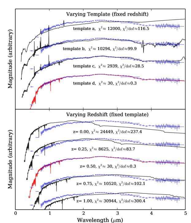
Figure 5.— A demonstration of the model-fitting procedure, using a small subset of the SED models in the grid. The high-resolution version of the model SEDs (thin lines), are plotted against an observed SED (blue points). The values of $\chi^{2}$ and $\chi^{2}$ per degree of freedom ($\chi^{2}/\rm dof$) are indicated. Upper panel: Four SED models with constant $z$, $E(B-V)$, and reddening law, but varying base template are compared with the observed fluxes. The best-fitting model is plotted in red. Lower panel: The template, $E(B-V)$, and reddening law are held constant, while $z$ is varied. The best-fitting model is plotted in red.

As discussed previously, the model grid is constructed using SED templates from Brown et al. (2014) and Salvato et al. (2011). For each of the 188 templates in our grid, we sample redshifts from 0–4.5 in steps of $dz=0.0015$, $E(B-V)$ values from 0–1 in steps of $dE(B-V)=0.045$, and five reddening laws, which means the model grid contains 55,146,667 model SEDs. The expected fluxes of each model in the grid are pre-computed by integrating the high-resolution model against the SPHEREx LVF filter profiles and the PS1 + WISE filter profiles. These fluxes are then stored in a file prior to the model-fitting step.

Figure 5 shows a small sample of SED models in the model grid, compared with an observed SED. We have shown the high-resolution versions of the models so that the spectral features being probed are more obvious to the eye. The plot demonstrates how drastically $\chi^{2}$ varies with different model SEDs.

5.6. Implementation in AWS

The simulation code and input data files are stored in an Amazon Machine Image (AMI) so that the simulation can run in Amazon.com’s Elastic Compute Cloud (EC2). The AMI includes the StratOS software framework (Stickley & Aragon-Calvo, 2015), which can automatically build a virtual computing cluster from EC2 instances. The StratOS framework is used to execute the most computationally expensive parts of the simulation on the slave nodes of the virtual cluster, while less expensive tasks are typically performed on the master node. For example, in order to efficiently create the grid of model SEDs, the input data from the COSMOS catalog is partitioned into smaller sections, which are sent to the slave nodes for processing. While the slave nodes are busy generating the model grid, the master node creates synthetic images for each band, measures the fluxes from the images, and constructs a catalog of observed SEDs. For more details on the sub-components of the pipeline, refer to the Appendix.

The StratOS framework efficiently schedules the tasks running on the slave nodes, which prevents the simulation from being slowed down significantly by a small number of low-performing nodes (e.g., nodes running in EC2 instances that have shared tenancy). Without the sort of scheduling provided by StratOS, the performance of the simulation would be limited by the speed of the slowest slave node. The framework’s resilience to node failure also prevents work from being lost in the rare event of an EC2 host failure.

6. Conclusions

Using a detailed end-to-end simulation based on empirical data from the COSMOS survey, we have verified the ability of the all-sky SPHEREx mission to recover accurate redshifts to a sufficient number of galaxies to put important new constraints on cosmological parameters, in particular $f_{\rm NL}$. The realism of the simulation, which captures systematic instrument effects as well as confusion and noise due to galaxies below the SPHEREx detection limit, gives us significant confidence in the cosmological performance of the proposed SPHEREx mission.

Generally, we have demonstrated that deep, multiwaveband photometry of surveys such as COSMOS can be used to place highly realistic constraints on the expected performance of cosmology surveys. The empirically-driven, interpolative approach to simulating mission performance is preferable to pure simulations in that it captures all of the relevant factors with high fidelity. Important effects captured by the simulation include source confusion, noise due to faint sources below the detection limit, realistic galaxy SEDs, and representative emission line characteristics. The framework developed here for simulating mission performance of wide-area cosmology surveys is broadly applicable to studies of the performance of future missions such as LSST, Euclid, and WFIRST, and can be applied to the problem of predicting the performance of BAO and weak lensing cosmology with these missions with minor modifications.

7. Acknowledgements

Part of the research described in this paper was carried out at the Jet Propulsion Laboratory, California Institute of Technology, under a contract with the National Aeronautics and Space Administration. RdP and OD acknowledge the generous support of the Heising-Simons Foundation.

Appendix A Implementation details

The computationally intensive components of the simulation are implemented in three C++ programs, named fitcat, make-grid, and photo-z, while other tasks are primarily performed in interpreted languages (Python, Perl, and IDL). The C++ programs are all parallelized with OpenMP and are optimized for systems with non-uniform memory access (i.e., shared memory systems with multiple CPU sockets or multiple memory controllers). These programs operate on input files that can trivially be split into smaller pieces so that the work can easily be distributed over the nodes of a computing cluster. The IDL scripts are compatible with the free GNU Data Language interpreter, so no special licenses need to be purchased in order to run the code. The simulation is customized to run efficiently in Amazon’s Elastic Compute Cloud, as described in §5.6, however it can also run on a single Linux workstation without modification.

Most of the adjustable parameters in the pipeline are stored in a single parameter file. To run new simulations, the user typically only needs to modify the parameter file and possibly modify the data in the input files. The simulation code consists of 7 major steps:

Step 1: Input catalog model-fitting with fitcat

We begin by using fitcat to assign SED model parameters (tuples of template type, $E(B-V)$, and reddening law) to the objects in the COSMOS catalog, as discussed in §5.2. For each unique redshift in the COSMOS catalog, a grid of SED models is created. The models are integrated against the COSMOS filters so that they can be directly compared with the fluxes in the catalog. In order to identify the model which best fits an object in the catalog, we begin by noting the redshift of the object. We then fetch the grid of models corresponding to that redshift. The fluxes of each model in the grid are compared with the object’s fluxes and then the best-fitting model (i.e., the model which minimizes the $\chi^{2}$ difference) is identified. The parameters of the best-fitting model are then stored in an output catalog, along with the scaling factor by which the model was multiplied in order to minimize $\chi^{2}$. This step in the simulation only needs to be performed when the template library is updated or a new catalog becomes available.

Step 2: Instrument simulation

In the second step, engineering data and survey properties, such as the integration times and the physical dimensions of the instrument, are used to generate simulated LVF transmission curves and PSF size. Noise characteristics for each band are also computed during this step and lead to the full sky performances, described in Doré et al. (2014).

Step 3: Input photometry generation with make-grid

The make-grid program computes fluxes by integrating filter profiles against templates after first scaling, redshifting, and reddening the templates, as specified by an input file. Given 1) a template library, 2) a set of SPHEREx LVF filter transmission curves, and 3) the list of model parameters, identified in Step 1, make-grid computes SEDs for the objects in the COSMOS catalog, interpolated to the SPHEREx bands, as described in §5.2.

Step 4: Model grid generation with make-grid

We use make-grid to generate a large grid of models of varying redshift, template type, extinction, and reddening law, as described in §5.5. The models are integrated against the SPHEREx LVF transmission curves so that they can be directly compared with the observed SEDs later (in Step 7). The model grid is stored in a compact binary file format, optimized for fast reading.

This step is very computationally expensive. For example, a SPHEREx model grid containing $5.5\times 10^{7}$ models requires 150 CPU core-hours, on an Intel Ivy Bridge CPU, running at 2.7 GHz. Thus, this step is typically performed on a computing cluster while another computer performs Steps 5 and 6. Note that model grids can be saved and stored for later use; the grid only needs to be re-generated when changes are made to the instrument specifications or the template library.

Step 5: Image generation

For each of the SPHEREx LVF bands, a FITS image is generated, as described in §5.3, using the coordinate data in the COSMOS catalog, the fluxes computed in Step 3, and the PSF determined in Step 2. The images are generated using utilities included in IMCAT. The IMCAT utilities are not multi-threaded, so multiple processes are spawned simultaneously in order to accelerate the image generation process.

Step 6: Observed SED generation

The user can specify detection threshold magnitudes for various bands, based on the detection limits of the external survey that they are using to identify objects of interest. In the case of the SPHEREx simulation, the detection thresholds are given by the depths of the Pan-STARRS PS1 and WISE W1 and W2 bands. Objects that are brighter than at least one of these thresholds are marked as detectable. An IDL script then performs photometry measurements on each FITS image, as described in §5.4, using the PSFs computed in Step 2 and the known coordinates of the detectable objects. Once the fluxes have been measured, the data are re-organized to generate observed SEDs for each object that was marked as detectable.

Step 7: Photometric redshift estimation with photo-z

The photo-z program performs the photometric redshift estimation, described in §5.5. It reads the extracted SEDs (produced in Step 6) and the model grid, (generated in Step 4). The program then produces a catalog containing estimated redshifts as well as additional information about each redshift estimate. For example, the skewness and kurtosis of the liklihood distribution are reported along with the global minimum $\chi^{2}$ value and the ID number of the associated best-fitting template.

The photometric redshift estimation algorithm is computationally expensive, particularly when large model grids are used. For example, estimating the redshifts of $5.3\times 10^{4}$ objects with SEDs consisting of 100 bands, using a grid containing $5.5\times 10^{7}$ models requires approximately 260 CPU core-hours on a an Intel Ivy Bridge CPU, running at 2.7 GHz. The current implementation of photo-z requires the entire model grid to be loaded into system memory on each individual computing node. Thus, the size of the model grid is currently limited by the amount of memory (RAM) available in each individual node of the cluster. In a future (production-quality) version of the redshift estimation pipeline, the grid will likely be broken into several redshift-based partitions that are small enough to fit into the memory of a graphics processing unit (GPU). A cluster of GPUs would then compute the elements of the redshift liklihood distributions; the moments of the distributions would still be computed using a CPU-native code.

References

- Allen (1976) Allen, D. A. 1976, MNRAS, 174, 29P
- Arnouts et al. (1999) Arnouts, S., Cristiani, S., Moscardini, L., et al. 1999, MNRAS, 310, 540
- Arnouts & Ilbert (2011) Arnouts, S., & Ilbert, O. 2011, LePHARE: Photometric Analysis for Redshift Estimate, Astrophysics Source Code Library, ascl:1108.009
- Brown et al. (2014) Brown, M. J. I., Moustakas, J., Smith, J.-D. T., et al. 2014, ApJS, 212, 18
- Bruzual & Charlot (2003) Bruzual, G., & Charlot, S. 2003, MNRAS, 344, 1000
- Calzetti et al. (2000) Calzetti, D., Armus, L., Bohlin, R. C., et al. 2000, ApJ, 533, 682
- Capak et al. (2007) Capak, P., Aussel, H., Ajiki, M., et al. 2007, ApJS, 172, 99
- Chabrier et al. (2000) Chabrier, G., Baraffe, I., Allard, F., & Hauschildt, P. 2000, ApJ, 542, 464
- Coil et al. (2011) Coil, A. L., Blanton, M. R., Burles, S. M., et al. 2011, ApJ, 741, 8
- Cool et al. (2013) Cool, R. J., Moustakas, J., Blanton, M. R., et al. 2013, ApJ, 767, 118
- da Cunha et al. (2012) da Cunha, E., Charlot, S., Dunne, L., Smith, D., & Rowlands, K. 2012, in IAU Symposium, Vol. 284, The Spectral Energy Distribution of Galaxies - SED 2011, ed. R. J. Tuffs & C. C. Popescu, 292
- Doré et al. (2014) Doré, O., Bock, J., Ashby, M., et al. 2014, ArXiv e-prints, arXiv:1412.4872
- Elliott et al. (2016) Elliott, H. A., McComas, D. J., Valek, P., et al. 2016, ApJS, 223, 19
- Fitzpatrick & Massa (1986) Fitzpatrick, E. L., & Massa, D. 1986, ApJ, 307, 286
- Ilbert et al. (2009) Ilbert, O., Capak, P., Salvato, M., et al. 2009, ApJ, 690, 1236
- Kaiser (2004) Kaiser, N. 2004, in Proc. SPIE, Vol. 5489, Ground-based Telescopes, ed. J. M. Oschmann, Jr., 11
- Kaiser et al. (2002) Kaiser, N., Aussel, H., Burke, B. E., et al. 2002, in Proc. SPIE, Vol. 4836, Survey and Other Telescope Technologies and Discoveries, ed. J. A. Tyson & S. Wolff, 154
- Koekemoer et al. (2011) Koekemoer, A. M., Faber, S. M., Ferguson, H. C., et al. 2011, ApJS, 197, 36
- Laigle et al. (2016) Laigle, C., McCracken, H. J., Ilbert, O., et al. 2016, ApJS, 224, 24
- Laureijs et al. (2011) Laureijs, R., Amiaux, J., Arduini, S., et al. 2011, ArXiv e-prints, arXiv:1110.3193 [astro-ph.CO]
- Levi et al. (2013) Levi, M., Bebek, C., Beers, T., et al. 2013, ArXiv e-prints, arXiv:1308.0847 [astro-ph.CO]
- LSST Science Collaboration et al. (2009) LSST Science Collaboration, Abell, P. A., Allison, J., et al. 2009, ArXiv e-prints, arXiv:0912.0201 [astro-ph.IM]
- Masters et al. (2015) Masters, D., Capak, P., Stern, D., et al. 2015, ApJ, 813, 53
- McCracken et al. (2013) McCracken, H. J., Milvang-Jensen, B., Dunlop, J., et al. 2013, The Messenger, 154, 29
- Moles et al. (2008) Moles, M., Benítez, N., Aguerri, J. A. L., et al. 2008, AJ, 136, 1325
- Neugebauer et al. (1984) Neugebauer, G., Habing, H. J., van Duinen, R., et al. 1984, ApJ, 278, L1
- Prevot et al. (1984) Prevot, M. L., Lequeux, J., Prevot, L., Maurice, E., & Rocca-Volmerange, B. 1984, A&A, 132, 389
- Salvato et al. (2011) Salvato, M., Ilbert, O., Hasinger, G., et al. 2011, ApJ, 742, 61
- Scoville et al. (2007) Scoville, N., Aussel, H., Brusa, M., et al. 2007, ApJS, 172, 1
- Seaton (1979) Seaton, M. J. 1979, MNRAS, 187, 73P
- Smoot et al. (1992) Smoot, G. F., Bennett, C. L., Kogut, A., et al. 1992, ApJ, 396, L1
- Spergel et al. (2015) Spergel, D., Gehrels, N., Baltay, C., et al. 2015, ArXiv e-prints, arXiv:1503.03757 [astro-ph.IM]
- Stickley & Aragon-Calvo (2015) Stickley, N. R., & Aragon-Calvo, M. A. 2015, ArXiv e-prints, arXiv:1503.02233 [astro-ph.IM]
- Takada et al. (2014) Takada, M., Ellis, R. S., Chiba, M., et al. 2014, PASJ, 66, R1
- Wright et al. (2010) Wright, E. L., Eisenhardt, P. R. M., Mainzer, A. K., et al. 2010, AJ, 140, 1868