Universal power-law decay of electron-electron interactions due to nonlinear screening in a Josephson junction array

Abstract

Josephson junctions are the most prominent nondissipative and at the same time nonlinear elements in superconducting circuits allowing Cooper pairs to tunnel coherently between two superconductors separated by a tunneling barrier. Due to this, physical systems involving Josephson junctions show highly complex behavior and interesting novel phenomena. Here, we consider an infinite one-dimensional chain of superconducting islands where neighboring islands are coupled by capacitances. We study the effect of Josephson junctions shunting each island to a common ground superconductor. We treat the system in the regime where the Josephson energy exceeds the capacitive coupling between the islands. For the case of two offset charges on two distinct islands, we calculate the interaction energy of these charges mediated by quantum phase slips due to the Josephson nonlinearities. We treat the phase slips in an instanton approximation and map the problem onto a classical partition function of interacting particles. Using the Mayer cluster expansion, we find that the interaction potential of the offset charges decays with an universal inverse-square power law behavior.

I Introduction

In a circuit of capacitively coupled metallic islands, static screening describes the redistribution of polarization charges on the capacitive plates of the islands in response to a static offset charge on one of the islands. The resulting voltages are determined by a (screened) Poisson equation. The way in which the solution decays with the distance from the offset charge depends on the effective circuit dimensionality. In one-dimensional networks, the polarization charge generically is constant up to the screening length and then follows a purely exponential decay. For metallic islands coupled by capacitances $C$, the screening length $\sqrt{2C/C_{g}}$ is determined by the ratio of $C$ to the capacitances $C_{g}$ of the islands to ground.fazio:01

Josephson junctions in superconducting circuits add an interesting twist to the screening of static offset charge configurations. Conventional, linear inductances coupling two metal grains are normally not of interest since they invalidate the notion of islands with well-defined offset charges. In contrast, nonlinear Josephson inductances only allow tunneling of single Cooper-pairs such that offset charge cannot simply flow off an island contacted by a junction. While Josephson junctions formally leave charge quantization on the islands intact, charge quantization effects are effectively weakened by large quantum fluctuations of the charge when the charging energy $E_{C}$ of the islands is much smaller than the Josephson energy $E_{J}$. This gives rise to what we will in the following refer to as nonlinear screening, an effect that has been exploited very successfully in the transmon qubit koch:07 .

In the regime of dominating Josephson energy, the dynamics of a single junction is dominated by quantum phase slips corresponding to tunneling of the superconducting phase difference by $2\pi$. For one-dimensional chains of Josephson junctions coupling the islands, the effects of phase slips have been extensively studied theoretically both in infinite bradley:84 ; korshunov:86 ; korshunov:89 and finite matveev:02 ; Hekking13 ; ribeiro:14 ; vogt:15 networks in the past. There has also been considerable effort in studying these systems experimentally pop:10 ; manucharyan:12 ; ergul:13 . Although many junctions are present in these systems, the junctions are not strongly coupled such that the dynamics are dominated by independent phase-slip events of the individual junctions and interactions do not play a crucial role.

Figure 1: In a) we show a conventional one dimensional infinite chain of capacitors with capacitance $C$. Each island is connected to the ground by a capacitance $C_{g}$. There is a fixed bias charge $q_{0}$ on a single island, inducing charges on the neighboring capacitor plates. However, due to the ground capacitances there is an exponential screening of this charge along the chain. At each island a fraction of the induced charge is stored on the ground capacitance so that the charge on the coupling capacitances $C$ decays exponentially with the distance to the original bias charge. The system in b) is similar to the system in a) with a Josephson junction (Josephson energy $E_{J}$) providing an additional shunt to the ground. Induced charges can now also be screened by tunneling through the Josephson junction, giving rise to a novel nonlinear screening behavior.

While the nonlinear screening effected by a single Josephson junction as in the transmon is well-studied, the screening properties of systems of many junctions that are strongly coupled have not been investigated to the best of our knowledge. Motivated by the efficient screening of a single transmon, we therefore study a one-dimensional system of transmons that are strongly coupled by large capacitances $C$, see Fig. 1. This corresponds to a system of superconducting islands that are coupled by capacitances $C$ and shunted to ground by a Josephson junction with Josephson energy $E_{J}$ and associated capacitance $C_{g}$. We are interested in a regime of nonlinear screening dominated by the Josephson junctions which corresponds to a very small capacitance $C_{g}$ to ground with associated large (linear) screening length $\sqrt{2C/C_{g}}$. Phase slips dominate when the Josephson energy $E_{J}$ is much larger than the energy $E_{C}=e^{2}/2C$ associated with a nonzero voltage with respect to the ground on a single island. We will show below that the nonlinear screening due to the Josephson junctions leads to a universal power-law decay of the electron-electron interaction with power two. This implies a power-law decay of the polarization charge markedly different from the conventional exponential decay obtained for static screening due to capacitances.

The outline of the paper is as follows. In Sec. II, we introduce the problem and its corresponding imaginary-time partition function in the path-integral formulation. We discuss the dilute instanton-gas approximation in Sec. III and introduce the equal-time action that is accumulated when slips of the island phases by $2\pi$ occur simultaneously on different islands in Sec. IV. In Sec. V, we use the equal-time action to compute the action of an arbitrary tunneling path of the island phases. The corresponding partition function maps onto a classical (interacting) partition function which we compute using a Mayer expansion. We use these results in Sec. VI to compute the ground state energy. We discuss the consequences for charge screening in Sec. VII and conclude with a short discussion of our results.

II Setup and Model

The system of interest is shown in Fig. 1b). We analyze an infinite one-dimensional chain of superconducting islands with the superconducting phase $\varphi_{j}$ on the $j$-th island. The islands are coupled by capacitances $C$ and connected to the ground by a Josephson junction with Josephson energy $E_{J}$ and a capacitance $C_{g}$ in parallel. This gives charges the possibility to tunnel on and off the island, changing the screening behavior of the chain. We treat the problem within the quantum statistical path integral approach to calculate the partition function $Z$ of the system. As the phase-variables of the islands are compact and defined only on the circle $[0,2\pi)$ it is useful to introduce the winding number $n_{j}\in\mathbb{Z}$ for the $j$-th island. With this, we can split the path integral for each phase $\varphi_{j}$ into sectors containing paths that wind $n_{j}$ times around the circle. For the full partition function, we have to sum over all closed paths corresponding to all possible winding numbers. Additionally, we have to integrate over the starting positions $\phi_{j}$. Hence, the partition function is given by

$$Z=\prod_{j}\Biggl{(}\sum_{n_{j}}\int_{0}^{2\pi}\!d\phi_{j}\int_{\begin{subarray}{l}\varphi_{j}=\phi_{j}\end{subarray}}^{\varphi_{f}=\phi_{j}+2\pi n_{j}}\mathcal{D}[\varphi_{j}]\Biggr{)}e^{-S/\hbar},$$ (1)

where we have introduced the Euclidean action $S=\int_{0}^{\beta}\!d\tau\;(L_{C}+L_{q})$ with the inverse temperature $\beta=\hbar/k_{B}T$. The Lagrangian $L_{C}$ corresponding to the circuit without bias charges is given by

$$L_{C} =\sum_{j=-\infty}^{\infty}\Bigl{\{}\frac{\hbar^{2}}{16E_{C_{g}}}\dot{\varphi}_{j}^{2}+\frac{\hbar^{2}}{16E_{C}}(\dot{\varphi}_{j+1}-\dot{\varphi}_{j})^{2}$$

$$\quad-E_{J}[1-\cos(\varphi_{j})]\Bigr{\}},$$ (2)

where $\dot{\varphi}_{i}=d\varphi_{i}/d\tau$. The first term in the sum describes the capacitive coupling to the ground, the second term the coupling between the islands, and the last term the Josephson junctions with Josephson energy $E_{J}$ connecting the islands to the ground. The energy scales of the capactive terms are given by $E_{C_{g}}=e^{2}/2C_{g}$ and $E_{C}=e^{2}/2C$. To study the screening effect of the system in the presence of bias charges on selected islands, we need the additional Lagrangian

$$L_{q}=\sum_{j=-\infty}^{\infty}\frac{i\hbar}{2e}q_{j}\dot{\varphi}_{j}$$ (3)

which implements the bias charges $q_{j}$ on the $j$-th island. This term is special for two reasons: On one hand, it is a total time derivative and thus does not enter the classical equations of motion. On the other hand, it is imaginary so that it only adds a phase to the partition function underlining its nonclassicality.

From the free energy $F=-\hbar\log(Z)/\beta$, we can calculate the ground state energy $E$ of the system by applying the low temperature limit

$$E=\lim_{\beta\rightarrow\infty}F.$$ (4)

The aim of this work is to calculate this ground state energy as a function of two bias charges and use it to gain information about the screening behavior of the chain.

III Partition function

We are in particular interested in the regime where $E_{C}\ll E_{J}\ll E_{C_{g}}$ so that the conventional capacitance to the ground $C_{g}$ is very small and the Josephson junctions are mainly responsible for any charge screening on the islands. From the fact that $E_{J}/E_{C}\gg 1$, we know that the ground state of the system will be well-localized in the phase variables $\varphi_{j}$. Therefore, the main contributions in (1) are due to paths starting and ending in the minimum of the cosine potentials. As we are only interested in exponential accuracy for the calculation of the ground state energy with (4), we can set $\phi_{j}=0$ and omit the integral over $\phi_{j}$. We are left with the evaluation of

$$Z_{0}=\prod_{j}\Biggl{(}\sum_{n_{j}}\int_{\begin{subarray}{l}\varphi_{j}=0\end{subarray}}^{\varphi_{f}=2\pi n_{j}}\mathcal{D}[\varphi_{j}]\Biggr{)}e^{-S_{C}/\hbar+i\pi\bm{n}\cdot\bm{q}/e}.$$ (5)

Here, the action $S_{C}$ is $S_{C}=\int_{0}^{\beta}d\tau\,L_{C}$ and we have already carried out the time integral over the term

$$\int_{0}^{\beta}\!d\tau\;L_{q} =\frac{i\hbar}{2e}\sum_{j}q_{j}\int_{0}^{\beta}\!d\tau\;\dot{\varphi}_{j}=\frac{i\hbar\pi}{e}\;\bm{n}\cdot\bm{q}$$ (6)

due to the bias charges. The vector $\bm{n}$ with components $n_{j}$ encodes the winding sector and $\bm{q}$ with components $q_{j}$ is the vector of bias charges. As we are analyzing a regime where the phases are good variables, fluctuations around the classical paths defined by the solutions of the Euler-Lagrange equations (corresponding to $L_{C}$) are small. Hence, we apply an instanton approximation where we replace the path integral by a sum over all classical solutions, while quantum fluctuations around the classical paths play just a sub-dominant role. In general, the main contribution to these fluctuations arise from Gaussian integration of the action expanded to second order around the classical paths. We assume that the fluctuations can be factorized so that they simply renormalize the bare parameters. This amounts to introducing the weight prefactor $K(\bm{n},\varphi_{\text{cl}})$, accounting for the fluctuations. By summing over all saddle point solutions of the Euler Lagrange equations $\{\varphi_{\text{cl}}(\bm{n})\}$, the partition function in the instanton approximation reads

$$Z_{0}=\sum_{\bm{n}}\sum_{\{\varphi_{\text{cl}}(\bm{n})\}}K(\bm{n},\varphi_{\text{cl}})e^{-S_{\text{cl}}[\varphi_{\text{cl}}]/\hbar+i\pi\bm{n}\cdot\bm{q}/e},$$ (7)

where $S_{\text{cl}}[\varphi_{\text{cl}}]$ is the action corresponding to the classical path $\varphi_{\text{cl}}(\bm{n})$.

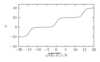
Figure 2: A possible saddle-point solution of the of equations of motion for a single island with phase variable $\varphi$. Every step (phase slip) in the curve is described by an instanton particle localized in time. The action corresponding to such a path can be approximated by the action of a single phase slip times the number of total phase slips. This is possible because the constant parts of the steps do not contribute to the action.

An example of such a simple path for just a single island (only one $n_{j}$ is different from 0) is shown in Fig. 2. The fact that we analyze the semi-classical regime where the phase is well-localized allows to use the dilute instanton gas approximation. The approximation holds as the phase-slip rate is so small that the phase slips (instantons) are well separated from each other, i.e., there is at most a single phase slip present within the duration $\tau_{0}=\hbar/\sqrt{E_{J}E_{C}}$ of a single phase-slip process. Thus, the classical paths consist of almost instantaneous individual phase slips that are well-separated in (imaginary) time. These phase slips are centered at their occurrence times $\tau_{j}$ for the $j$-th phase slip. In between the phase slips, the phase stays constant. In that way, we treat paths with more than a single phase slip at the same island as independent phase slips, i.e., there is no temporal interaction between the instantons. As a consequence the total action is simply the sum of individual instanton contributions Coleman85 . However, simultaneous phase slips at different islands cannot be treated independently because they are subject to a spatial interaction due to the coupling between the islands. Therefore, this case needs special treatment that we deal with in the next section.

In principle we also have to calculate the prefactor $K(\bm{n})$ due to the fluctuations around the classical action. These fluctuations are not important when it comes to exponential accuracy. However, due to time translation invariance, in the single instanton sector, the second-order integration for the fluctuations additionally contains an integration of a zero mode, corresponding to a simple shift of the full instanton solution in time. We separate the prefactor $K(\bm{n})=\tilde{K}(\bm{n})\beta$ into a factor $\tilde{K}(\bm{n})$ containing the real fluctuations on one side and the imaginary time interval $\beta$ resulting from the zero mode integration on the other side. Thus, every contribution is weighted by the fluctuations $\tilde{K}(\bm{n})$ and the length of the time intervall $\beta$ in which we consider the evolution of the system. For a single instanton on a single island, which is a noninteracting problem, it is known that $\tilde{K}\simeq 1/\tau_{0}$ (compare, e.g., to Refs. koch:07, ; pop:10, ; matveev:02, ). However, as the precision of this prefactor is not as important as the precision for the exponentiated instanton action we assume the single instanton value $1/\tau_{0}$ to be sufficient even for the interacting problem with many simultaneous instantons at different islandsSethna81 . This approximation is appropriate because the terms become smaller with the number of instantons such that in the end only prefactors $\tilde{K}$ with a moderate amount of instantons are relevant.

IV Equal-Time Action

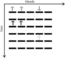
Figure 3: Example configuration of the system where we have sliced the time dimension into a lattice to better visualize the finite time an instanton process needs. The arrows pointing up correspond to instantons, while the arrows pointing down correspond to anti-instantons. (Anti-)instantons occurring at the same time are subject to a spatial interaction (here marked by the same gray scale) and add a contribution to the full action given by their equal-time action. For the full partition function, we need to sum over all possible configurations. To that end, we consider each phase slip event at an island as a particle with the island position, occurrence time and instanton type as generalized coordinates. In this picture, evaluating the full partition function corresponds to calculating the the classical grand-canonical partition function of the particles.

Considering a single island with a single phase variable, the dilute instanton gas approximation allows to treat the different phase slips (in imaginary time) independently. However, in our problem we have many interacting phase degrees of freedom (in space) rendering the situation more involved. Therefore, in this section, we determine the irreducible equal-time action $S_{\text{ET}}$ including the simultaneous phase-slip processes explicitly. For a proper definition of the equal-time action, we use the fact that within a time interval of size $\tau_{0}$ there can be at most a single phase slip per island. Together with the diluteness of the instanton gas, it is convenient to define the equal-time action as the action picked up by the total system in a time window $\tau_{0}$ around a given time $\tau^{*}$. In this context it is useful to imagine the (imaginary) time to be discrete with a temporal lattice constant $\tau_{0}$. Figure 3 illustrates an example configuration on such a lattice. For the calculation of $S_{\text{ET}}$ at the time $\tau^{*}$, we only need the information which of the phases execute a (anti-)phase slip. Later on, we will employ the equal-time action in the limit of short instanton processes $\tau_{0}\rightarrow 0$, which applies in our regime of interest, to construct the full action by adding the different contributions independently in accordance with the dilute gas approximation.

In principle, for the explicit calculation of $S_{\text{ET}}$ at time $\tau^{*}$, we need to extract the part of the classical paths matching the time window of size $\tau_{0}$ around $\tau^{*}$ and insert this into the Lagrangian. However, as the phase slips are almost instantaneous, we are only interested whether a particular island $j$ exhibits a phase slip ($n^{*}_{j}=1)$, an anti phase slip ($n^{*}_{j}=-1$) or no phase slip ($n^{*}_{j}=0$) at time $\tau^{*}$. Moreover, since the system does not pick up any action as long as the phases are constant, we can extend the time-integration from minus infinity to plus infinity as the phases are only nonconstant for the short time interval $\tau_{0}$ around $\tau^{*}$. This yields $S_{\text{ET}}=\int_{-\infty}^{\infty}\!d\tau\;L_{C1}(\tau)$, where $L_{C1}$ is the circuit Lagrangian with the classical solution for a single phase slip per phase inserted. The boundary conditions are provided by

$$\varphi_{j}(\tau)=2\pi\begin{cases}m_{j}^{*},&\tau<\tau^{*}-\tau_{0}/2,\\ m_{j}^{*}+n_{j}^{*},&\tau>\tau^{*}+\tau_{0}/2.\end{cases}$$ (8)

Here, the discrete variable $m_{j}^{*}\in\mathbb{Z}$ contains the information about the phase before the time interval of size $\tau_{0}$ around $\tau^{*}$.

The task is the calculation of the classical action for an interacting nonlinear system that in general cannot be carried out exactly. Therefore, we introduce an approximation to the nonlinear Josephson cosine potential by replacing it by a periodic parabolic potential called the Villain approximationVillain75 , i.e., $1-\cos(\varphi_{j})\approx\text{min}_{m_{j}}(\varphi_{j}-2\pi m_{j})^{2}/2$ with $m_{j}\in\mathbb{Z}$. Taking the minimum with respect to the discrete variable $m_{j}$ corresponds to taking the phases modulo $2\pi$. In the case of no phase slip with $n_{j}^{*}=0$ this means $m_{j}=m_{j}^{*}$ independent of the time. However, in the case of $n_{j}^{*}=\pm 1$ we have $m_{j}=m_{j}^{*}$ for $\tau<\tau^{*}$ and $m_{j}=m_{j}^{*}+n_{j}^{*}$ for $\tau>\tau^{*}$. This can be summarized for all cases as

$$m_{j}(\tau)=m_{j}^{*}+n_{j}^{*}\Theta(\tau-\tau^{*}),$$ (9)

where $\Theta(\tau)$ is the Heaviside theta function. With the Euler-Lagrange equations for the Villain potential, it is straightforward to show that the Lagrangian $L_{C1}$ is mirror symmetric with respect to the time $\tau^{*}$. Thus it is sufficient to calculate the action for times before $\tau^{*}$ and double the result yielding $S_{\text{ET}}=2\int_{-\infty}^{\tau^{*}}\!d\tau L_{C}(\tau)$. Additionally, the symmetry provides the boundary condition $\varphi_{j}(\tau^{*})=\pi(m_{j}^{*}+n_{j}^{*})$.

Except from the bias charge term that does not change the classical equations of motion, the system is translationally invariant and thus can be diagonalized by the Fourier transform

$$\varphi_{j} =\frac{1}{2\pi}\int_{0}^{2\pi}\!dk\;e^{ikj}\varphi_{k}, \varphi_{k} =\sum_{j}e^{-ikj}\varphi_{j}.$$ (10)

Expressing the circuit Lagrangian $L_{C1}$ for $\tau\leq\tau^{*}$ in terms of $\varphi_{k}$ gives rise to

$$L_{C1}=\frac{1}{2\pi}\int\!dk\; \biggl{\{}\frac{\hbar^{2}}{16E_{C_{\Sigma}}}\biggl{[}1-\frac{\cos(k)}{1+\varepsilon^{2}}\biggr{]}|\dot{\varphi}_{k}|^{2}$$

$$+E_{J}/2|\varphi_{k}|^{2}\biggr{\}},$$ (11)

where $E_{C_{\Sigma}}=e^{2}/2(C_{g}+2C)$ is the full charging energy and

$$\varepsilon=\sqrt{C_{g}/2C}$$ (12)

the inverse screening length. At this point we make use of the fact that the Hamiltonian corresponding to $L_{C}$ is a conserved quantity. For the instanton, it is equal to zero because the instantons correspond to saddle-point solutions in the minima of the potentials. The conservation of the Hamiltonian directly yields

$$\frac{\hbar^{2}}{16E_{C_{\Sigma}}}\biggl{[}1-\frac{\cos(k)}{1+\varepsilon^{2}}\biggr{]}|\dot{\varphi}_{k}|^{2}=\frac{E_{J}}{2}|\varphi_{k}|^{2}.$$ (13)

With this equation, we can express the equal-time action as

$$S_{\text{ET}}(\bm{n}^{*}) =2\int_{-\infty}^{\tau^{*}}\!d\tau\;L_{C1}$$

$$=\int\!\frac{dk}{\pi}\!\int_{0}^{\pi n_{k}^{*}}\!d|\varphi_{k}|\sqrt{\frac{E_{J}}{8E_{C_{\Sigma}}}\biggl{[}1-\frac{\cos(k)}{1+\varepsilon^{2}}\biggr{]}}|\varphi_{k}|$$

$$=\int\!dk\;U(k)|n_{k}^{*}|^{2},$$ (14)

with $U(k)=\pi\sqrt{[1-\cos(k)/(1+\varepsilon^{2})]E_{J}/32E_{C_{\Sigma}}}$ and $n_{k}^{*}$ the Fourier transform of $n_{j}^{*}$. In real space, we obtain the expression

$$S_{\text{ET}}(\bm{n}^{*}) =\sum_{i,j}\;n_{i}^{*}U(i-j)n_{j}^{*},$$ (15)

where $U(j)$ is the Fourier transform of $U(k)$. For small $\varepsilon$ an accurate approximation for the real space potential can be given by

$$U(j) =\alpha\frac{2\varepsilon jK_{1}(2\varepsilon j)}{\tfrac{1}{4}-j^{2}}\approx\alpha\frac{1}{\tfrac{1}{4}-j^{2}}\quad(\text{for }\varepsilon\ll 1).$$ (16)

Here, $K_{1}$ is the first modified Bessel function of the second kind with $K_{1}(x)\approx 1/x$ for $x\ll 1$. Hence the potential shows an inverse-square decay until it reaches the screening length $\varepsilon^{-1}$ and turns into an exponential decay. The coupling strength is given by

$$\alpha=\pi\sqrt{E_{J}/8E_{C}}.$$ (17)

Note that the equal-time action of interacting instantons can be fully described by the two-particle interaction $U(j)$ between all corresponding instantons. Additionally, we want to highlight that though the equal-time action describes the action picked up at a selected time it does not explicitly depend on the time but only on the underlying instanton configuration $\bm{n}$.

With the action at a given moment in time, we can proceed to calculate the full action for a specific instanton configuration within the dilute gas approximation. In the next section, we are going to use the equal-time action to calculate the partition function by summing over all instanton configurations $\bm{n}$ and integrating over all times the instantons occur; this step is analogous to going over from a first to a second quantized description of the problem.

V Ground State Energy

We now turn to the estimation of the ground state Energy $E$. As a first step, we calculate the full partition function $Z_{0}$. With the instanton approximation and the equal-time action in real space, this is equivalent to a classical interacting statistical mechanics problem. To make this correspondence clearer, we introduce a particle picture for the phase slips. The general task is to evaluate (7) in the dilute gas approximation, which means summing over all configurations of instantons on all islands at all possible times. In the particle picture, the sum over all configurations is realized by a sum over all numbers of instanton particles together with the sum over the generalized coordinate $x_{a}$ of every particle $a=1,\dots,N$. The generalized coordinate $x_{a}$ of every particle includes its island coordinate $r_{a}\in\mathbb{Z}$, the time $\tau_{a}$, and the instanton type $\sigma_{a}\in\{+,-\}$ (instanton or anti-instanton) . Hence, such an instanton particle corresponds to a single phase slip at a specific time and location. We use the shorthand notation

$$\int dx_{a}=\sum_{r_{a},\sigma_{a}}\int_{0}^{\beta}\!\frac{d\tau_{a}}{\tau_{0}}\;$$ (18)

to express the summation over all configurations of the $a$-th particle. With that, we can rewrite (7) as

$$Z_{0} =\sum_{N=0}^{\infty}\frac{z^{N}}{N!}\int\!dx_{1}\cdots dx_{N}$$

$$\qquad\quad\times\exp\biggl{[}{-\sum_{\makebox[17.50003pt]{$\scriptstyle 1\leq a<b\leq N$}}V_{a,b}+i\sum_{1\leq a\leq N}\pi\sigma_{a}q(r_{a})/e}\biggr{]},$$ (19)

which is a classical partition function in the grand canonical ensemble. Note that the factor $N!$ prevents overcounting of the configurations. The fugacity $z$ is defined by the self-interaction part of Eq. (15) (with $a=b$) of a single instanton with $z=\exp[{-U(0)}]$. In this context we can interpret $z/\tau_{0}$ as the instanton rate. As $z\ll 1$ there will be much less than a single instanton per time $\tau_{0}$ on average, justifying the dilute gas approximation. The rest of the interacting part is absorbed in the interaction potential

$$V_{a,b}=\begin{cases}\infty,\hskip 2.0pt&r_{a}=r_{b},|\tau_{a}-\tau_{b}|\lesssim\tau_{0}/2\\ 2\sigma_{a}U(r_{a}-r_{b})\sigma_{b},\hskip 2.0pt&r_{a}\neq r_{b},|\tau_{a}-\tau_{b}|\lesssim\tau_{0}/2\\ 0,\hskip 5.0pt&\text{else}.\end{cases},$$ (20)

We implement the potential as a hardcore potential, so that only a single phase slip can happen on a given island at a given time. For phase slips occurring at different times, the interaction potential is zero because in the dilute gas approximation a spatial interaction between phase slips is only included for simultaneously events as explained in section IV. The bias charge part is implemented by the single particle potential $\pi\sigma_{a}q(r_{a})/e$, where $q(r)$ is the charge distribution over the islands.

The free energy corresponding to such an interacting partition function can be evaluated perturbatively in $z$ by the Mayer cluster expansion Mayer41 . The idea is to rewrite

$$e^{-V_{a,b}}=1+f_{a,b},$$ (21)

so that we split the contribution in noninteracting part and interacting part. The interacting part $f_{a,b}$ is, in the limit $\tau_{0}\rightarrow 0$, proportional to a Dirac delta function Note1 $\tau_{0}\delta(\tau_{a}-\tau_{b})$ with the width $\tau_{0}$. This again reflects the fact that in a dilute gas spatial interaction affects only simultaneous instantons. For large distances $|r_{a}-r_{b}|$, the interacting part $f_{a,b}$ is negligibly small, hence suggesting an expansion in the number of interacting particles. We can proceed similar with the bias charge potential. Here, we consider only two charges separated by $M$ with the charge distribution $q(r)=q_{0}\delta_{r,0}+q_{M}\delta_{r,M}$. We can write

$$e^{i\pi\sigma_{a}q(r_{a})/e} =\exp({i\pi\sigma_{a}q_{0}\delta_{r_{a},0}/e})\exp({i\pi\sigma_{a}q_{M}\delta_{r_{a},M}/e})$$

$$=(1+g_{0,a})(1+g_{M,a}),$$ (22)

where $g_{a,b}=\exp[i\pi\sigma_{b}q_{a}\delta_{r_{b},a}/e]-1$ expresses the interaction of phase slip $b$ with the charge on island $a$. Using these relations, the partition function assumes the form

$$Z_{0}=\sum_{N=0}^{\infty}\frac{z^{N}}{N!} \int\!dx_{1}\cdots dx_{N}$$

$$\times\prod_{\begin{subarray}{c}a<b\\ l\end{subarray}}(1+f_{a,b})(1+g_{0,l})(1+g_{M,l}),$$ (23)

where the part in the product of the partition function contains terms with different numbers of $f$ functions like

$$\prod_{a<b}(1+f_{a,b}) =[1+(f_{1,2}+f_{1,3}+\cdots)$$

$$\quad+(f_{1,2}f_{1,3}+f_{1,2}f_{1,4}+\cdots)+\cdots]$$ (24)

and similar for the $g$ functions. A simple way to keep track the terms appearing in the expansion is given by a diagrammatic approach: For every particle coordinate $x_{a}$ in an $n$-particle term we draw a circle (node) with the particle label $a$ inside. If an $f$-function $f_{a,b}$ is part of the term, we connect the $a$-th and $b$-th circle by a straight line (link). A $g_{0/M,l}$ is accounted for with a wiggled line starting from the $l$-th circle and ending in a circle with the corresponding label $q_{0}$ or $q_{M}$. In the end, we have to carry out a $dx_{a}$ integral for every node. Connected nodes represent interacting cluster of particles, which means that the integration of connected coordinates (clusters) is not necessarily independent, while nonconnected parts of the diagrams can be integrated independently.

Figure 4: The contributions to the cluster variables $b_{1}$ and $b_{2}$ as given in Eq. (V). The first-order diagrams in $b_{1}$ contain no spatial interaction at all, while the last diagram in $b_{2}$ mediates an interaction between the charges $q_{0}$ and $q_{M}$. The factor of 2 in front of some of the diagrams is due to the fact that these contributions can additionally be realized with the labels $1$ and $2$ interchanged.

It is important to realize that the value of such clusters after the integration does not depend on their labels, but only on the cluster topology and the number of coordinates included. Thus, we introduce the cluster variables $b_{j}$ given by

$$b_{1} =\frac{1}{1!\,L}\int\!dx_{1}\;(1+g_{0,1}+g_{M,1}),$$

$$b_{2} =\frac{1}{2!\,L}\int\!dx_{1}dx_{2}\;f_{1,2}\;[1+g_{0,1}+g_{M,1}+g_{0,2}+g_{M,2}$$

$$\qquad\qquad+g_{0,1}g_{M,2}+g_{0,2}g_{M,1}+g_{0,1}g_{0,2}+g_{M,1}g_{M,2}],$$

$$\qquad\qquad\qquad\vdots$$ (25)

where $L$ is the number of islands in the system so that $b_{n}$ is a finite quantity that includes all connected diagrams with $n$ particles and all their possible interactions with the bias charges. Terms corresponding to a single phase slip that are interacting with two charges at different islands do not contribute and thus terms involving $g_{0,a}g_{M,a}$ vanish. In Fig. 4 we show the diagrams corresponding to $b_{1}$ and $b_{2}$.

Every term in (V) consists of different numbers of one, two, three and more-particle clusters. A term including $m_{1}$ single-particle clusters, $m_{2}$ two-particle clusters and so on contains $N$ particles with $N=\sum_{j}m_{j}j$. It contributes

$$T =C(1!\,Lb_{1})^{m_{1}}(2!\,Lb_{2})^{m_{2}}(3!\,Lb_{3})^{m_{3}}\cdots,$$

$$C =\frac{N!}{[(1!)^{m_{1}}(2!)^{m_{2}}\cdots][m_{1}!\,m_{2}!\cdots]}$$ (26)

where the Faà di Bruno coefficient $C$ counts the number of ways of partitioning the $N$ particles into the different particle clusters. The sum over the instanton number $N$ in (V) translates into a sum over all cluster numbers $m_{i}$. Finally, we arrive at the expression for the partition function

$$Z_{0}=\lim_{L\rightarrow\infty}\sum_{m_{1},m_{2},\dots}\biggl{[}\frac{(Lzb_{1})^{m_{1}}}{m_{1}!}\frac{(Lz^{2}b_{2})^{m_{2}}}{m_{2}!}\cdots\biggr{]}$$ (27)

and hence with (4) the ground state energy is given by

$$E=\lim_{\begin{subarray}{c}\beta\rightarrow\infty\\ L\rightarrow\infty\end{subarray}}\Bigl{(}-\frac{L\hbar}{\beta}\sum_{l}b_{l}z^{l}\Bigr{)}.$$ (28)

This is an expansion in the fugacity $z$, where the order $l$ corresponds to the maximum number of particle clusters we take into account. Truncating the series at order 2 for example does not mean that we consider only terms with two instantons but that we only take interactions between pairs of instantons into account. In other words, we treat the system as a sum of many two-body problems. For small $z\ll 1$, like in our case of $E_{J}/E_{C_{\Sigma}}\gg 1$, such a truncation is justified.

We analyze an infinite system and therefore the extensive energy $E$, scaling with the system size $L$, diverges. As we are interested in charge screening, we split the ground state energy

$$E=\mathcal{E}_{0}L+E_{1}(q_{0})+E_{1}(q_{M})+E_{2}(q_{0},q_{M}),$$ (29)

where $\mathcal{E}_{0}$ is the energy density accounting for the bias charge nonrelated energy per island that is stored in the chain. From the latter, corresponding to all diagrams without a bias charge circle, we can in principle get information about the pressure and other thermodynamic variables in the system. However, here we are only interested in the influence due to the bias charges. The parts including information about these break the translational invariance of the chain and therefore do not scale with the system size. This gives rise to the two energies $E_{1}(q)$ and $E_{2}(q_{1},q_{2})$, where the first provides the change in the ground state energy due to a single charge and the latter corresponds to the interaction energy between two charges.

VI Single Charge and Interaction Energy

We proceed by evaluating the ground state energy. First, we want to calculate the ground state energy dependency on a single bias charge corresponding to $E_{1}(q_{0})$. In our case, it is enough to consider the first order in (28), because the second order is already suppressed by an additional factor of the fugacity $z$. The task is to calculate the part of $b_{1}$ corresponding to $E_{1}(q_{0})$. The diagrammatic expansion makes it easy to select the correct terms. There is only a single diagram that we have to take into account: A single particle circle connected to a single bias charge $q_{0}$ (Fig. 4, the second diagram in $b_{1}$), which is given by the simple expression

$$b_{1}(q_{0}) =\frac{1}{1!\,L}\int\!dx_{1}\;g_{0,1},$$

$$=\frac{\beta}{L\tau_{0}}(e^{i\pi q_{0}/e}-1)+(e^{-i\pi q_{0}/e}-1)$$

$$=\frac{2\beta}{L\tau_{0}}[\cos(\pi q_{0}/e)-1].$$ (30)

As the $g$-functions are zero everywhere expect at the island where the corresponding charge is located, they act as Kronecker-Delta and project the whole sum over the instanton coordinate on the location of the bias charge. From $b_{1}$, we find

$$E_{1}(q_{0}) =\frac{2\hbar}{\tau_{0}}e^{-\pi\sqrt{2E_{J}/E_{C}}}[1-\cos(\pi q_{0}/e)].$$ (31)

This energy is similar to known results for problems with only single junctions (see e.g. koch:07, ). The exponent is slightly different from the conventional scaling $\sqrt{8E_{J}/E_{C_{g}}}$ as every junction in the chain, different from single junction systems, is coupled to other junctions. If we redid the calculation in the limit $\varepsilon\rightarrow\infty$, which turns off the coupling between the islands, and scale $E_{J}\mapsto(8/\pi^{2})^{2}E_{J}$ to compensate an error due to the Villain approximation Hekking13 , we would recover the known result.

The next step is the calculation of the interaction energy $E_{2}(q_{0},q_{M})$. Here, it is not enough to consider only first-order terms in (28), because single-instanton diagrams can only contain single charges. Thus, the leading order of the interaction energy is given by the two-instanton diagrams where every particle circle is connected to a charge circle (the last contribution in $b_{2}$ in Fig. 4) corresponding to the expression

$$b_{2}(q_{0},q_{M}) =\frac{1}{2!\,L}\int\!dx_{1}dx_{2}\;2f_{1,2}g_{0,1}g_{M,2}.$$ (32)

By considering solely the terms depending on both charges in the result for $b_{2}(q_{0},q_{M})$, we find the interaction energy

$$E_{2}(q_{0},q_{M}) =\frac{2\hbar}{\tau_{0}}e^{-2\pi\sqrt{2E_{J}/E_{C}}}$$

$$\quad\times\biggl{\{}\Bigl{[}e^{-2U(M)}-1\Bigr{]}\cos[\pi(q_{0}+q_{M})/e]$$

$$\quad\quad+\Bigl{[}e^{2U(M)}-1\Bigr{]}\cos[\pi(q_{0}-q_{M})/e]\biggr{\}}.$$ (33)

For large enough $M$, we have $U(M)\ll 1$ and can therefore expand the interaction energy in $U$ with the result

$$E_{2}\approx\frac{8\hbar}{\tau_{0}}e^{-2\pi\sqrt{2E_{J}/E_{C}}}U(M)\sin(\pi q_{0}/e)\sin(\pi q_{M}/e).$$ (34)

In this approximation, the charge interaction is directly proportional to the instanton-interaction $U(M)$ and obeys a decay proportional to the inverse-square distance between the charges (below the screening length).

VII Charge Screening

In the final section, we return to the original question about the charge screening effect of Josephson junctions. In a first step, we treat the case of a single bias charge $q_{0}$ on island $0$. The presence of a charge on an island induces an average charge on neighboring capacitor plates. To calculate the latter we need to know the average voltages $V_{M}$ at the different islands ($M\neq 0$). We can handle this task by using the results (31) and (34) and employing linear response theory. The derivative of the ground state energy with respect to an external parameter gives the average value of the derivative of the action with respect to the same parameter. From (3) and (4) and the time translation invariance in the system, we obtain that the voltages $V_{M}$ are given by the derivative of the ground state energy $E$ with respect to the bias charge. To this end, we shift the bias charges on the $M$-th island such that the ground state energy $E(q_{0},\delta_{M})$ depends on the small shift $\delta_{M}$. We then find

$$\frac{\partial E(q_{0}+\delta_{0},\delta_{M})}{\partial\delta_{M}}\bigg{|}_{\delta_{0},\delta_{M}=0} =\frac{i\hbar}{2e}\langle\dot{\varphi}_{M}\rangle=V_{M};$$ (35)

here, in order to determine the voltages expectation values $V_{M}$ on island $M$, we have used the Josephson relation $d\varphi_{M}/dt=2eV_{M}/\hbar$ together with the relation $\tau=it$ between real and imaginary time.

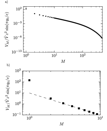
Figure 5: Double logarithmic plots of the voltage $V_{M}$ induced on island $M$ by an offset charge at distance $M$ for $E_{J}/E_{C}=5$ and $\varepsilon=0.01$. In panel a), we show the full result corresponding to Eq. (36). The screened voltage follows a power-law behavior until the screening length is reached at which point the exponential screening due to the ground capacitances $C_{g}$ takes over. In b) we compare the result obtained by using the power-law approximation (VII) represented by the dashed line with the black squares representing the full result. It can be seen that the decay of the induced voltages follows the inverse-square law essentially starting from $M=2$.

The leading contribution to $E(q_{0}+\delta_{0},\delta_{M})$ is given by the interaction energy $E_{2}(q_{0}+\delta_{0},\delta_{M})$ of (VI). Taking the derivative, we obtain the result ($\tilde{V}=2\pi\hbar/e\tau_{0}$)

$$V_{M} =\tilde{V}e^{-2\pi\sqrt{2E_{J}/E_{C}}}\Bigl{[}e^{-2U(M)}-e^{2U(M)}\Bigr{]}\sin(\pi q_{0}/e),$$ (36)

which can be approximated by the expression

$$V_{M} \approx-4\tilde{V}e^{-2\pi\sqrt{2E_{J}/E_{C}}}U(M)\sin(\pi q_{0}/e)$$

$$\approx\frac{4\tilde{V}\alpha e^{-2\pi\sqrt{2E_{J}/E_{C}}}\sin(\pi q_{0}/e)}{M^{2}}.$$ (37)

By expanding the exponential in (36) we see that all even orders cancel so that there are no corrections until the third order in $U(M)$. This makes the approximation (VII) already accurate for $M>\sqrt{2\alpha-1/4}$, where the exponent is smaller than 1. Even in the regime of our interest $E_{J}\gg E_{C}$, $M$ does not have to be too large as $\alpha$ scales with the square root of $E_{J}/E_{C}$. Hence for intermediate distances (smaller than the screening length $\varepsilon^{-1}$, larger than $\sqrt{2\alpha-1/4}$) the voltages obey a universal inverse-square decay given by $U(M)$. In Figure 5 we show a plot of the decay of the induced voltages. Note that an additional charge can be treated by adding up the voltage contributions of every single charge. Deviations from this simple rule are induced by a three particle interaction-energy at least. Such contributions appear in three-instanton diagrams or higher and thus they are strongly suppressed. For completeness, we provide also the expression for the voltage on the $0$-th island

$$V_{0}=\tilde{V}e^{-\pi\sqrt{2E_{J}/E_{C}}}\sin(\pi q_{0}/e),$$ (38)

obtained from $E\approx E_{1}(q_{0}+\delta_{0})$.

With the voltages at hand, it is a simple task to determine the charges on all capacitor plates. From the relation for capacitors $C(V_{M}-V_{M+1})=Q_{M}$, the charge on the capacitor plate on the right of the $M$-th island (relative to the bias charge) $Q_{M}$ is simply proportional to the voltage difference over the capacitance. The largest voltage difference can be found between the bias charge island and its two direct neighbors. Here we have to take the difference of the first order contribution (38) and the second-order contribution (36), where the latter is suppressed by $z$. Thus, the two capacitor plates directly attached to the bias charge island are charged the most. From the second island on, we only need to take differences of (36). This results in the power law decay

$$Q_{M}\approx\frac{8C\tilde{V}\alpha e^{-2\pi\sqrt{2E_{J}/E_{C}}}\sin(\pi q_{0}/e)}{M^{3}}.$$ (39)

for $1\ll M\ll\epsilon^{-1}$. The result is thus fundamentally different from an exponential decay in usual linear screening.

VIII Conclusion

In this work, we have calculated the effect of Josephson junctions on the charge screening in the ground state of an one-dimensional chain of capacitively coupled superconducting islands in the semi-classical limit $E_{J}/E_{C}\gg 1$. We have solved the problem of the interacting nonlinear system by using an instanton approximation within the quantum statistical path integral approach. To deal with the interactions in the chain, we have introduced the equal-time action corresponding to the action picked up by the whole system at a given moment in time. The latter includes spatial correlations between simultaneous phase slips on different islands. With this action and a dilute instanton gas approximation, which applies in the regime of interest, we have mapped the task of solving the quantum system onto a classical statistical mechanics problem. With a slightly modified Mayer cluster expansion, supporting the interaction with bias charges at selected islands of the chain, we have calculated a power series of the ground state energy $E(q_{0},q_{M})$ in the number of interacting instantons as a function of two bias charges $q_{0}$ and $q_{M}$. We have calculated the average induced voltages in the linear response regime and furthermore the induced charges on the capacitor plates. Compared to the known exponential decay for chains without the Josephson junctions, we have found that the induced voltages decay with the inverse of the squared distance. This power-law decay is fundamentally different from the conventional exponential screening. The effect arises due to interacting quantum phase slips through the nonlinear Josephson potentials of the Josephson junctions.

IX Acknowledgments

The authors acknowledge support from the Alexander von Humboldt foundation and the Deutsche Forschungsgemeinschaft (DFG) under grant HA 7084/2-1.

References

- (1) R. Fazio and H. van der Zant, Quantum phase transitions and vortex dynamics in superconducting networks, Phys. Rep. 355, 235 (2001).
- (2) J. Koch, T. M. Yu, J. Gambetta, A. A. Houck, D. I. Schuster, J. Majer, A. Blais, M. H. Devoret, S. M. Girvin, and R. J. Schoelkopf, Charge insensitive qubit design derived from the Cooper pair box, Phys. Rev. A 76, 042319 (2007).
- (3) R. M. Bradley and S. Doniach, Quantum fluctuations in chains of josephson junctions, Phys. Rev. B 30, 1138 (1984).
- (4) S. E. Korshunov, Collisionless friction mechanism for linear defects in quantum crystals, Sov. Phys. JETP 63, 1242 (1986).
- (5) S. E. Korshunov, Transition to the superfluid state of a step on a free surface of a quantum crystal, Sov. Phys. JETP 68, 1250 (1989).
- (6) K. A. Matveev, A. I. Larkin, and L. I. Glazman, Persistent current in superconducting nanorings, Phys. Rev. Lett. 89, 096802 (2002).
- (7) G. Rastelli, I. M. Pop, and F. W. J. Hekking, Quantum phase slips in Josephson junction rings, Phys. Rev. B 87, 174513 (2013).
- (8) P. Ribeiro and A. M. García-García, Interplay of classical and quantum capacitance in a one-dimensional array of Josephson junctions, Phys. Rev. B 89, 064513 (2014).
- (9) N. Vogt, R. Schäfer, H. Rotzinger, W. Cui, A. Fiebig, A. Shnirman, and A. V. Ustinov, One-dimensional Josephson junction arrays: Lifting the Coulomb blockade by depinning, Phys. Rev. B 92, 045435 (2015).
- (10) I. M. Pop, I. Protopopov, F. Lecocq, Z. Peng, B. Pannetier, O. Buisson, and W. Guichard, Measurement of the effect of quantum phase-slips in a Josephson junction chain, Nature Phys. 6, 589 (2010).
- (11) V. E. Manucharyan, N. A. Masluk, A. Kamal, J. Koch, L. I. Glazman, and M. H. Devoret, Evidence for coherent quantum phase-slips across a Josephson junction array, Phys. Rev. B 85, 024521 (2012).
- (12) A. Ergül, J. Lidmar, J. Johansson, Y. Azizoğlu, D. Schaeffer, and D. Haviland, Localizing quantum phase slips in one-dimensional josephson junction chains, New J. Phys. 15, 095014 (2013).
- (13) S. Coleman, The uses of instantons (Cambridge University Press, 1985).
- (14) J. P. Sethna, Phonon coupling in tunneling systems at zero temperature: An instanton approach, Phys. Rev. B 24, 698 (1981).
- (15) Villain, J., Theory of one- and two-dimensional magnets with an easy magnetization plane. ii. the planar, classical, two-dimensional magnet, J. Phys. France 36 (6), 581 (1975).
- (16) J. E. Mayer and E. Montroll, Molecular distribution, J. Chem. Phys. 9 (1), 2 (1941).
- (17) If the diagram in question contains loops, one of the in every loop should not be written proportional to a Dirac delta function in time. The constraint of simultaneous phase slips for interacting processes is already fulfilled by the other lines connecting the loop.