Forward-backward envelope for the sum of two nonconvex functions: further properties and nonmonotone line-search algorithms

Abstract.

We propose ZeroFPR, a nonmonotone linesearch algorithm for minimizing the sum of two nonconvex functions, one of which is smooth and the other possibly nonsmooth. ZeroFPR is the first algorithm that, despite being fit for fully nonconvex problems and requiring only the black-box oracle of forward-backward splitting (FBS) — namely evaluations of the gradient of the smooth term and of the proximity operator of the nonsmooth one — achieves superlinear convergence rates under mild assumptions at the limit point when the linesearch directions satisfy a Dennis-Moré condition, and we show that this is the case for quasi-Newton directions. Our approach is based on the forward-backward envelope (FBE), an exact and strictly continuous penalty function for the original cost. Extending previous results we show that, despite being nonsmooth for fully nonconvex problems, the FBE still enjoys favorable first- and second-order properties which are key for the convergence results of ZeroFPR. Our theoretical results are backed up by promising numerical simulations. On large-scale problems, by computing linesearch directions using limited-memory quasi-Newton updates our algorithm greatly outperforms FBS and its accelerated variant (AFBS).

1. Introduction

In this paper we deal with optimization problems of the form

(1) $$\minimize_{x\in\R^{n}}\ \varphi(x)\equiv f(x)+g(x)$$

under the following assumptions, which will be valid throughout the paper without further mention. [Basic assumption]In problem (1)

1. $f\in C^{1,1}(\R^{n})$ (differentiable with $L_{f}$-Lipschitz continuous gradient);

2. $\func{g}{\R^{n}}{\Rinf}$ is proper, closed and $\gamma_{g}$-prox-bounded (see Section 2.1);

3. a solution exists, that is, $\argmin\varphi\neq\emptyset$.

Both $f$ and $g$ are allowed to be nonconvex, making (1) prototypic for a plethora of applications spanning signal and image processing, machine learning, statistics, control and system identification. A well known algorithm addressing (1) is forward-backward splitting (FBS), also known as proximal gradient method. FBS has been thoroughly analyzed under the assumption of $g$ being convex. If moreover $f$ is convex, then FBS is known to converge globally with rate $O(1/k)$ in terms of objective value, where $k$ is the iteration count. In this case, accelerated variants of FBS, also known as fast forward-backward splitting (FFBS), can be derived thanks to the work of Nesterov [8, 32], that only require minimal additional computations per iteration but achieve the provably optimal global convergence rate of order $o(1/k^{2})$ [6].

The work in [36] pioneered an alternative acceleration technique. The method is based on an exact, real-valued penalty function for the original problem (1), namely the forward-backward envelope (FBE), defined as follows

(2) $$\varphi_{\gamma}(x){}={}\varphi_{\gamma}^{f,g}(x){}\coloneqq{}\inf_{z\in\R^{n}}\set{f(x)+\tinnprod{\nabla f(x)}{z-x}+\tfrac{1}{2\gamma}\|z-x\|^{2}+g(z)}$$

where $\gamma>0$ is a given parameter. We will adopt the simpler notation $\varphi_{\gamma}$ without superscript whenever $f$ and $g$ are clear from the context.

The name forward-backward envelope comes from the fact that $\varphi_{\gamma}(x)$ is the value of the minimization problem that defines the forward-backward step and alludes to the kinship that it has with the Moreau envelope. These claims will be addressed more in detail in Section 4. When $f$ is sufficiently smooth and both $f$ and $g$ are convex, the FBE was shown to be continuously differentiable and amenable to be minimized with generalized Newton methods. More recently, [45] proposed a linesearch algorithm based on (L-)BFGS quasi-Newton directions for minimizing the FBE. The curvature information exploited by Newton-like methods acts as an online preconditioner, enabling superlinear rates of convergence under mild assumptions. However, unlike plain (F)FBS schemes, such methods require accessing second-order information of the smooth term $f$ (needed for the evaluation of $\nabla\varphi_{\gamma}$), and are well defined only as long as the nonsmooth term $g$ is convex. On the contrary, FBS merely requires first-order information on $f$ and prox-boundedness of the nonsmooth term $g$, in which case all accumulation points are stationary for $\varphi$, they satisfy the first order necessary conditions [5].

Contributions

In this paper we propose ZeroFPR, a nonmonotone linesearch algorithm that, to the best of our knowledge, is the first that (1) addresses the same range of problems as FBS, (2) requires the same black-box oracle as FBS (gradient of one function and proximity operator of the other), (3) yet achieves superlinear rates under mild assumptions (only) at the limit point. Though related to minFBE algorithm [45], ZeroFPR is conceptually different, mainly because it is gradient-free, in the sense that it does not require the gradient of the FBE. Moreover,

• We provide the necessary theoretical background linking the concepts of stationarity of a point for problem (1), criticality and optimality. To the best of our knowledge, such an analysis was previously made only for the proximal point algorithm [40] and for a special case of the projected gradient method [7].

• The analysis of the FBE, previously studied only in the case of $f$ being $C^{2}(\R^{n})$ and $g$ convex [45], is extended to $f$ and $g$ as in Equation 1. In particular, we provide mild assumptions on $f$ and $g$ that ensure (1) continuous differentiabilty of the FBE around critical points, (2) (strict) twice differentiability at critical points, and (3) equivalence of strong local minimality for the original function and the FBE.

• Exploiting the investigated properties of the FBE and of critical points we prove that ZeroFPR with monotone linesearch converges (1) globally if $\varphi_{\gamma}$ has the Kurdyka-Łojasiewicz property [29, 30, 24], and (2) superlinearly when quasi-Newton Broyden directions are employed, under mild additional requirements at the limit point.

Organization of the paper

In Section 2 we introduce some notation and list some known facts about FBS. In Section 3 we define and explore notions of stationarity and criticality for the investigated problem and relate them with properties of the forward-backward operator. In Section 4 we extend the results of [45] about the fundamental properties of the FBE to the more general setting addressed in this paper, where $f$ and $g$ satisfy Equation 1; for the sake of readability, some of the proofs are deferred to Appendix A. Section 5 addresses the core contribution of the paper, ZeroFPR; although arbitrary directions can be chosen, we specialize the results on superlinear convergence to a quasi-Newton Broyden method so as to truely maintain the same black-box oracle as FBS. Some ancillary results needed for the proofs are listed in Appendix B. Finally, Section 6 illustrates numerical results obtained with the proposed method.

2. Preliminaries

2.1. Notation

The identity $n\times n$ matrix is denoted as $\id$, and the extended real line as $\Rinf=\R\cup\set{\infty}$. The open and closed ball of radius $r\geq 0$ centered in $x\in\R^{n}$ is denoted as $\ball xr$ and $\cball xr$, respectively. Given a set $E$ and a sequence $\seq{x^{k}}$ we write $\seq{x^{k}}\subset E$ with the obvious meaning of $x^{k}\in E$ for all $k\in\N$. The (possibly empty) set of cluster points of $\seq{x^{k}}$ is denoted as $\omega\left(\seq{x^{k}}\right)$, or simply as $\omega(x^{k})$ whenever the indexing is clear from the context. We say that $\seq{x^{k}}\subset\R^{n}$ is summable if $\sum_{k\in\N}\|x^{k}\|$ is finite, and square-summable if $\seq{\|x^{k}\|^{2}}$ is summable.

Following the terminology of [44], we say that a function $\func{f}{\R^{n}}{\R}$ is strictly continuous at $\bar{x}$ if $\limsup_{\begin{subarray}{c}y,z\to\bar{x}\\ y\neq z\end{subarray}}{\frac{|f(y)-f(z)|}{\|y-z\|}}$ is finite, and strictly differentiable at $\bar{x}$ if $\nabla f(\bar{x})$ exists and $\lim_{\begin{subarray}{c}y,z\to\bar{x}\\ y\neq z\end{subarray}}{\frac{f(y)-f(z)-\innprod{\nabla f(\bar{x})}{y-z}}{\|y-z\|}}{}={}0$. The set of functions $\R^{n}\to\R$ with Lipschitz continuous gradient is denoted as $C^{1,1}(\R^{n})$, and for $f\in C^{1,1}(\R^{n})$ we write $L_{f}$ to indicate the Lipschitz modulus of $\nabla f$.

For a proper, closed function $\func{g}{\R^{n}}{\Rinf}$, a vector $v\in\partial g(x)$ is a subgradient of $g$ at $x$, where the subdifferential $\partial g(x)$ is considered in the sense of [44, Def. 8.3]

$$\partial g(x){}={} \set{v\in\R^{n}}[\exists\seq{x^{k}}\to x,\seq{v^{k}\in\hat{\partial}g(x^{k})}\to v\leavevmode\nobreak\ \text{s.t.}\leavevmode\nobreak\ g(x^{k})\to g(x)],$$

and $$\hat{\partial}g(x) g x$$ is the set of regular subgradients of at , namely

$$\hat{\partial}g(x){}={} \set{v\in\R^{n}}[g(z)\geq g(x){}+{}\innprod{v}{z-x}{}+{}o(\|z-x\|),\leavevmode\nobreak\ \forall z\in\R^{n}\vphantom{\seq{x^{k}}}].$$

We have $\partial\varphi(x){}={}\nabla f(x){}+{}\partial g(x)$ and $\hat{\partial}\varphi(x){}={}\nabla f(x){}+{}\hat{\partial}g(x)$ [44, Ex. 8.8(c)].

Given a parameter value $\gamma>0$, the Moreau envelope function $g^{\gamma}$ and the proximal mapping $\prox_{\gamma g}$ are defined by

(3) $$g^{\gamma}(x){}\coloneqq{} \inf_{z}\set{g(z)+\tfrac{1}{2\gamma}\|z-x\|^{2}},$$

(4) $$\prox_{\gamma g}(x){}\coloneqq{} \argmin_{z}\set{g(z)+\tfrac{1}{2\gamma}\|z-x\|^{2}}.$$

We now summarize some properties of $g^{\gamma}$ and $\prox_{\gamma g}$; the interested reader is referred to [44] for a detailed discussion. A function $\func{g}{\R^{n}}{\Rinf}$ is prox-bounded if there exists $\gamma>0$ such that $g+\tfrac{1}{2\gamma}\|{}\cdot{}\|^{2}$ is bounded below on $\R^{n}$. The supremum of all such $\gamma$ is the threshold $\gamma_{g}$ of prox-boundedness for $g$. In particular, if $g$ is convex or bounded below then $\gamma_{g}=\infty$. In general, for any $\gamma\in(0,\gamma_{g})$ the proximal mapping $\prox_{\gamma g}$ is nonempty- and compact-valued, and the Moreau envelope $g^{\gamma}$ finite [44, Thm. 1.25].

Given a nonempty closed set $S\subseteq\R^{n}$ we let $\func{\indicator_{S}}{\R^{n}}{\Rinf}$ denote its indicator function, namely $\indicator_{S}(x)=0$ if $x\in S$ and $\indicator_{S}(x)=\infty$ otherwise, and $\ffunc{\proj_{S}}{\R^{n}}{\R^{n}}$ the (set-valued) projection $x\mapsto\argmin_{z\in S}\|z-x\|$. Proximal mappings can be seen as generalized projections, due to the relation $\proj_{S}=\prox_{\gamma{\indicator_{S}}}$ for any $\gamma>0$.

For a set-valued mapping $\ffunc{T}{\R^{n}}{\R^{n}}$ we let $\graph T=\set{(x,y)}[y\in T(x)]$ denote its graph, $\zer T=\set{x\in\R^{n}}[0\in T(x)]$ the set of its zeros and $\fix T=\set{x\in\R^{n}}[x\in T(x)]$ the set of its fixed-points.

2.2. Forward-backward iterations

Due to the quadratic upper bound

(5) $$f(z){}\leq{}f(x)+\tinnprod{\nabla f(x)}{z-x}+\tfrac{L_{f}}{2}\|z-x\|^{2}$$

holding for all $x,z\in\R^{n}$ [9, Prop. A.24], for any $\gamma\in(0,\nicefrac{{1}}{{L_{f}}})$ the function

(6) $$\ell_{\gamma}^{f,g}\left(z;\,x\right){}\coloneqq{}f(x)+\innprod{\nabla f(x)}{z-x}+\tfrac{1}{2\gamma}\|z-x\|^{2}+g(z)$$

furnishes a majorization model for $\varphi$, in the sense that

• $\ell_{\gamma}^{f,g}\left(\fillwidthof[l]{x}{z};\,x\right)\geq\varphi(\fillwidthof[l]{x}{z})$ for all $x,z\in\R^{n}$, and

• $\ell_{\gamma}^{f,g}\left(x;\,x\right)=\varphi(x)$ for all $x\in\R^{n}$.

Given a point $x\in\R^{n}$, one iteration of forward-backward splitting (FBS) for problem (1) consists in the minimization of the majorizing function $\ell_{\gamma}^{f,g}$, namely, in selecting

(7) $$x^{+}{}\in{}T_{\gamma}^{f,g}(x){}\coloneqq{}\fillwidthof[l]{\FB x,}{{\argmin}_{z}\ell_{\gamma}^{f,g}\left(z;\,x\right),}$$

where $\gamma\in\bigl{(}0,\min\set{\gamma_{g},\nicefrac{{1}}{{L_{f}}}}\bigr{)}$ is the stepsize parameter. The (set-valued) forward-backward operator $T_{\gamma}^{f,g}$ can be equivalently expressed as

(8a) $$\hphantom{x^{+}\in{}}T_{\gamma}^{f,g}(x){}={} \FB x,$$

which motivates the bound $$\gamma<\gamma_{g} x^{+} x$$ in (7) to ensure the existence of for any . We also introduce the corresponding (set-valued) forward-backward residual, namely

(8b) $$\hphantom{x^{+}\in{}}R_{\gamma}^{f,g}(x){}\coloneqq{} \fillwidthof[l]{\FB x,}{\tfrac{1}{\gamma}\bigl{(}x-T_{\gamma}^{f,g}(x)\bigr{)}.}$$

Whenever no ambiguity occurs, we will omit the superscript and write simply $\ell_{\gamma}$, $T_{\gamma}$ and $R_{\gamma}$ in place of $\ell_{\gamma}^{f,g}$, $T_{\gamma}^{f,g}$ and $R_{\gamma}^{f,g}$, respectively.

(7) emphasizes that FBS is a majorization-minimization algorithm (MM), a class of methods which has been thoroughly analyzed when the majorizing function is strongly convex in the first argument [13] (for $\ell_{\gamma}$, this is the case when $g$ is convex). MM algorithms are of interest whenever minimizing the surrogate function $\ell_{\gamma}\left({}\cdot{};\,x\right)$ is significantly easier than directly addressing the non structured minimization of $\varphi$. For FBS this translates into simplicity of $\prox_{\gamma g}$ and $\nabla f$ operations, cf. (8a). Under very mild assumptions FBS iterations (7) converge to a critical point (see Section 3) independently of the choice of $x^{+}$ in the set $T_{\gamma}(x)$ [5]. The key is the following well known sufficient decrease property, whose proof can be found in [12, Lem. 2]. [Sufficient decrease]For any $\gamma\in(0,\gamma_{g})$, $x\in\R^{n}$ and $\bar{x}\in T_{\gamma}(x)$ it holds that $\varphi(\bar{x}){}\leq{}\varphi(x){}-{}\tfrac{1-\gamma L_{f}}{2\gamma}\|x-\bar{x}\|^{2}$.

3. Stationary and critical points

Unless $\varphi$ is convex, the stationarity condition $0\in\hat{\partial}\varphi(x^{\star})$ in problem (1) is only necessary for the optimality of $x^{\star}$ [44, Thm. 10.1]. In this section we define different concepts of (sub)optimality and show how they are related for generic functions $\varphi=f+g$ as in Equation 1. We say that a point $x^{\star}\in\dom\varphi$ is

1. stationary if $0\in\hat{\partial}\varphi(x^{\star})$;

2. critical if it is $\gamma$-critical for some $\gamma\in(0,\gamma_{g})$, if $x^{\star}\in T_{\gamma}(x^{\star})$;

3. optimal if $x^{\star}\in\argmin\varphi$, if it solves (1).

The notion of criticality was already discussed in [7] under the name of $L$-stationarity ($L$ plays the role of $\nicefrac{{1}}{{\gamma}}$) for the special case of $g=\indicator_{B\cap C_{s}}$, where $B$ is a convex set and $C_{s}$ is the (nonconvex) set of vectors with at most $s$ nonzero entries.

If $g$ is convex, then $\gamma_{g}=\infty$ and we may talk of criticality without mention of $\gamma$: in this case, the properties of $\gamma$-criticality and stationarity are equivalent regardless of the value of $\gamma$. For more general functions $g$, instead, the value of $\gamma$ plays a role in determining whether a point is $\gamma$-critical or not, which legitimizes the following definition. The criticality threshold is the function $\func{\Gamma^{f,g}}{\R^{n}}{[0,\gamma_{g}]}$

(9) $$\Gamma^{f,g}(x){}\coloneqq{}\sup\bigl{(}\set{\gamma>0}[{x\in T_{\gamma}^{f,g}(x)}]\cup\set{0}\bigr{)}\quad\text{for $x\in\R^{n}$.}$$

As usual, whenever $f$ and $g$ are clear from the context we simply write $\Gamma$ in place of $\Gamma^{f,g}$. That $\Gamma\leq\gamma_{g}$ is due to the fact that $\prox_{\gamma g}$ (and consequently $T_{\gamma}$) is everywhere empty-valued for $\gamma>\gamma_{g}$. Considering also $\gamma=0$ forces the set in the definition to be nonempty, and the lower-bound $\Gamma\geq 0$ in particular; more precisely, observe that, by definition, $\Gamma(x)>0$ iff $x$ is a critical point.

Let us consider $\varphi=f+g$ for $f(x)=\frac{1}{2}x^{2}$ and $g=\indicator_{C}$ where $C=\set{\pm 1}$. Clearly, $\gamma_{g}=+\infty$ (as $g$ is lower-bounded), $L_{f}=1$ and $\pm 1$ are both (unique) optima. Since $\hat{\partial}\varphi(x)=\R$ for $x\in C$ and $\hat{\partial}\varphi$ is clearly empty elsewhere, all points in $C$ are stationary. $\prox_{\gamma g}$ is the (set-valued) projection on $C$, therefore the forward-backward operator is $T_{\gamma}(x){}={}\proj_{C}((1-\gamma)x)$. We have

$$T_{\gamma}(-1){}={}\begin{cases}[@{\!}c@{\leavevmode\nobreak\ \leavevmode\nobreak\ \text{if }}l@{}]\set{-1}&\gamma<1\\ \set{\pm 1}&\gamma=1\\ \set{1}&\gamma>1\end{cases}\quad\text{and}\quad T_{\gamma}(1){}={}\begin{cases}[@{\!}c@{\leavevmode\nobreak\ \leavevmode\nobreak\ \text{if }}l@{}]\set{1}&\gamma<1\\ \set{\pm 1}&\gamma=1\\ \set{-1}&\gamma>1.\end{cases}$$

In particular, $\Gamma(1)=\Gamma(-1)=1$. We now list some properties of critical and optimal points which will be used to derive regularity properties of $T_{\gamma}$ and $g^{\gamma}$. [Properties of critical points]The following properties hold:

1. for $\gamma\in(0,\gamma_{g})$, a point $x^{\star}$ is $\gamma$-critical iff

   $$g(x){}\geq{}g(x^{\star}){}+{}\innprod{-\nabla f(x^{\star})}{x-x^{\star}}{}-{}\tfrac{1}{2\gamma}\|x-x^{\star}\|^{2}\qquad\forall x\in\R^{n};$$

2. if $x^{\star}$ is critical, then it is $\gamma$-critical for all $\gamma\in(0,\Gamma(x^{\star}))$; moreover, $x^{\star}$ is also $\Gamma(x^{\star})$-critical provided that $\Gamma(x^{\star})<\gamma_{g}$;

3. $T_{\gamma}(x^{\star}){=}\set{x^{\star}}$ and $R_{\gamma}(x^{\star}){=}\set{0}$ for any critical point $x^{\star}$ and $\gamma\in(0,\Gamma(x^{\star}))$.

• 1: by definition, $x^{\star}$ is $\gamma$-critical iff $\ell_{\gamma}\left(x^{\star};\,x^{\star}\right)\leq\ell_{\gamma}\left(x;\,x^{\star}\right)$ for all $x$, iff

  $$f(x^{\star}){}+{}g(x^{\star}){}\leq{}f(x^{\star}){}+{}\innprod{\nabla f(x^{\star})}{x-x^{\star}}{}+{}\tfrac{1}{2\gamma}\|x-x^{\star}\|^{2}{}+{}g(x)\qquad\forall x\in\R^{n}.$$

  By suitably rearranging, the claim readily follows.

• 2: due to 1, if $x^{\star}$ is $\gamma$-critical, apparently it is also $\gamma^{\prime}$-critical for any $\gamma^{\prime}\in(0,\gamma]$. From the definition (9) of the criticality threshold $\Gamma(x^{\star})$, it then follows that $x^{\star}$ is $\gamma$-critical for any $\gamma\in(0,\Gamma(x^{\star}))$. Suppose now that $\Gamma(x^{\star})<\gamma_{g}$. Then, due to 1 for all $\gamma\in(0,\Gamma(x^{\star}))$ we have

  $$g(x){}\geq{}g(x^{\star}){}+{}\innprod{-\nabla f(x^{\star})}{x-x^{\star}}{}-{}\tfrac{1}{2\gamma}\|x-x^{\star}\|^{2}\quad\forall x\in\R^{n}.$$

  By taking the limit as $\gamma\nearrow\Gamma(x^{\star})$ we obtain that the inequality holds for $\Gamma(x^{\star})$ as well, proving the claim in light of the characterization 1.

• 3: let $x^{\star}$ be a critical point, and let $x\in T_{\gamma}(x^{\star})$ for some $\gamma<\Gamma(x^{\star})$. Fix $\gamma^{\prime}\in(\gamma,\Gamma(x^{\star}))$. From 1 and 2 it then follows that

  (10) $$g(x){}\geq{}g(x^{\star}){}+{}\innprod{-\nabla f(x^{\star})}{x-x^{\star}}{}-{}\tfrac{1}{2\gamma^{\prime}}\|x-x^{\star}\|^{2}.$$

  Since $x,x^{\star}\in T_{\gamma}(x^{\star})$, it holds that $\ell_{\gamma}\left(x^{\star};\,x^{\star}\right)=\ell_{\gamma}\left(x;\,x^{\star}\right)$,

  $$g(x^{\star}){}={}\innprod{\nabla f(x^{\star})}{x-x^{\star}}{}+{}\tfrac{1}{2\gamma}\|x-x^{\star}\|^{2}{}+{}g(x){}\overrel[\geq]{\eqref{eq:StrictInequality}}{}g(x^{\star}){}+{}\bigl{(}\tfrac{1}{2\gamma}-\tfrac{1}{2\gamma^{\prime}}\bigr{)}\|x-x^{\star}\|^{2}.$$

  Since $\tfrac{1}{2\gamma}-\tfrac{1}{2\gamma^{\prime}}>0$, necessarily $x=x^{\star}$.

The inequality in Item 1 can be rephrased as the fact that the vector $-\nabla f(\bar{x})$ is a “global” proximal subgradient for $g$ at $\bar{x}$ as in [44, Def. 8.45], where “global” refers to the fact that $\delta$ can be taken $+\infty$ in the cited definition. An interesting consequence is that the definition of criticality depends solely on $\varphi$ and not on the considered decomposition $f+g$; in fact, it is only the threshold $\Gamma$ that depends on it. To see this, let $\tilde{f}=f-h$ and $\tilde{g}=g+h$ for some $h\in C^{1,1}(\R^{n})$, and consider a point $x^{\star}$ which is $\gamma$-critical with respect to the decomposition $f+g$, such that $x^{\star}\in T_{\gamma}^{f,g}(x^{\star})$. Combining Item 1 with the quadratic bound (5) for $h$, we obtain

$$\smash{\tilde{g}}(x){}\geq{}\smash{\tilde{g}}(x^{\star}){}-{}\tinnprod{\nabla\smash{\tilde{f}}(x^{\star})}{x-x^{\star}}{}-{}\smash{\tfrac{1}{2\frac{\gamma}{1+\gamma L_{h}}}}\|x-x^{\star}\|^{2}\quad\text{for all $x\in\R^{n}$.}$$

Again from the characterization of Item 1, we deduce that $\smash{x^{\star}\in T_{\tilde{\gamma}}^{\tilde{f},\tilde{g}}(x^{\star})}$, where $\tilde{\gamma}{}={}\frac{\gamma}{1+\gamma L_{h}}$. In particular, considering $h=-f$ we infer that a point $x^{\star}$ is critical iff $x^{\star}\in T_{\gamma}^{0,\varphi}(x^{\star})=\prox_{\gamma\varphi}(x^{\star})$ for some $\gamma>0$, which legitimizes the notion of criticality without mentioning a specific decomposition.

In the next result we show that criticality is a halfway property between stationarity and optimality. In light of these relations we shall seek “suboptimal” solutions which we characterize as critical points. [Optimality, criticality, stationarity]Let $\bar{\gamma}{}\coloneqq{}\min\set{\gamma_{g},\nicefrac{{1}}{{L_{f}}}}$.

1. (criticality $\Rightarrow$ stationarity)  $\fix T_{\gamma}\subseteq\zer\hat{\partial}\varphi$ for all $\gamma\in(0,\gamma_{g})$;

2. (optimality $\Rightarrow$ criticality)  $\Gamma(x^{\star})\geq\bar{\gamma}$ for all $x^{\star}\in\argmin\varphi$; in particular, $\argmin\varphi\subseteq\fix T_{\gamma}$ for all $\gamma\in(0,\bar{\gamma})$, and also for $\gamma=\nicefrac{{1}}{{L_{f}}}$ if $\gamma_{g}>\nicefrac{{1}}{{L_{f}}}$;

• 1: let $\gamma\in(0,\gamma_{g})$ and $x\in\fix T_{\gamma}$. Since $x$ minimizes $g+\tfrac{1}{2\gamma}\|{}\cdot{}-x+\gamma\nabla f(x)\|^{2}$, we have $0{}\in{}\hat{\partial}\bigl{[}g+\tfrac{1}{2\gamma}\|{}\cdot{}-x+\gamma\nabla f(x)\|^{2}\bigr{]}(x){}={}\hat{\partial}g(x)+\nabla f(x){}={}\hat{\partial}\varphi(x)$, where the first inclusion follows from [44, Thm. 10.1] and the equalities from [44, Thm. 8.8(c)]. This proves that $x$ is stationary.

• 2: Fix $\gamma\in(0,\bar{\gamma})$, $x^{\star}\in\argmin\varphi$ and $y\in T_{\gamma}(x^{\star})$. Necessarily $y=x^{\star}$, otherwise, due to section 2.2, $\varphi(y)$ would contradict minimality of $\varphi(x^{\star})$. Therefore, $x^{\star}$ is $\gamma$-critical and the claim follows from the arbitrarity of $\gamma\in(0,\bar{\gamma})$.

As already seen in Section 3, the bound $\Gamma(x^{\star})\geq\min\set{\gamma_{g},\nicefrac{{1}}{{L_{f}}}}$ at optimal points in Item 2 is tight, and clearly the implication “optimality $\Rightarrow$ criticality” cannot be reversed (consider, the point $x^{\star}=0$ for $\varphi=\cos$). The next example shows that the other implication is also proper. [Stationarity $\not\Rightarrow$ criticality] Let $f(x)=\frac{1}{2}x^{2}$ and $g(x)=x^{\nicefrac{{5}}{{3}}}$. We have $\gamma_{g}=+\infty$, $L_{f}=1$, and for $x^{\star}=0$ it holds that $\hat{\partial}\varphi(x^{\star})=\set{\nabla\varphi(x^{\star})}=\set{0}$. Therefore, $x^{\star}$ is stationary; however, $T_{\gamma}(x^{\star})=\prox_{\gamma g}(0)=\set{-(\nicefrac{{5\gamma}}{{3}})^{3}}$, and in particular $x^{\star}\notin T_{\gamma}(x^{\star})$ for any $\gamma>0$, proving $x^{\star}$ to be non critical.

4. Forward-backward envelope

The FBE (2) was introduced in [36] and further analyzed in [45, 28] in the case when $g$ is convex. Under such assumption the FBE was shown to be continuously differentiable, which made it possible to derive minimization algorithms based on its gradient. In the general setting addressed in this paper the FBE might fail to be (continuously) differentiable, and as such we need to resort to gradient-free methods. This task will be addressed in Section 5 where Section 5 will be proposed; other than being applicable to a wider range of problems, the proposed scheme is entirely based on the same oracle of forward-backward iterations, unlike the approaches in [36, 45, 28] which instead require the computation of $\nabla^{2}f$. All this will be possible thanks to continuity properties of the FBE, and to the behavior of $\varphi_{\gamma}$ at critical points. We now focus on its continuity, while the other property will be addressed shortly after in Section 4.2.

[Alternative expressions for $\varphi_{\gamma}$] By expanding the square and rearranging the terms in the definition (2), $\varphi_{\gamma}$ can equivalently be expressed as

$$\varphi_{\gamma}(x){}={}\inf_{z\in\R^{n}}\set{f(x){}-{}\tfrac{\gamma}{2}\|\nabla f(x)\|^{2}{}+{}g(z){}+{}\tfrac{1}{2\gamma}\|z-x+\gamma\nabla f(x)\|^{2}}.$$

Comparing with (7), it is apparent that the set of minimizers $z$ in the above expression coincides with $T_{\gamma}(x)$, the forward-backward operator at $x$. Moreover, taking out the constant term $f(x){}-{}\tfrac{\gamma}{2}\|\nabla f(x)\|^{2}$ from the infimum we immediately obtain the following expression involving the Moreau envelope of $g$:

(11) $${\qed}\varphi_{\gamma}(x){}={}f(x){}-{}\tfrac{\gamma}{2}\|\nabla f(x)\|^{2}{}+{}g^{\gamma}(x-\gamma\nabla f(x)).$$

Other than providing an explicit way of computing the FBE, (11) emphasizes how $\varphi_{\gamma}$ inherits the regularity properties of the Moreau envelope of $g$. In particular, the next key property follows from the strict continuity of $g^{\gamma}$ [44, Ex. 10.32]. [Strict continuity of $\varphi_{\gamma}$]For any $\gamma\in(0,\gamma_{g})$, the FBE $\varphi_{\gamma}$ is a real-valued and strictly continuous function on $\R^{n}$.

4.1. Connections with the Moreau envelope

For the special case $f=0$, FBS iterations (7) reduce to the proximal point algorithm (PPA) $x^{+}\in\prox_{\gamma\varphi}(x)$, first introduced in [31] for convex functions $\varphi$ and later generalized for functions with convex majorizing surrogate $\ell_{\gamma}^{\,0,\varphi}\left({}\cdot{};\,x\right){}={}\varphi({}\cdot{})+\frac{1}{2\gamma}\|{}\cdot{}-x\|^{2}$, see [23]. Similarly, the FBE reduces to the Moreau envelope $\varphi^{\gamma}=\varphi_{\gamma}^{0,\varphi}$. In fact, the FBE extends the connection between PPA and Moreau envelope

(12a) $$\varphi^{\gamma}(x){}={} {\min}_{z}\ell_{\gamma}^{\,0,\varphi}\left(z;\,x\right) \quad\leftrightarrow\quad \prox_{\gamma\varphi}(x){}={}{\argmin}_{z}\ell_{\gamma}^{\,0,\varphi}\left(z;\,x\right),$$

holding for $$f=0 \ell_{\gamma}^{f,g} f\in C^{1,1}(\R^{n})$$ in (6), to majorizing functions with arbitrary

(12b) $$\varphi_{\gamma}(x){}={} {\min}_{z}\ell_{\gamma}^{f,g}\left(z;\,x\right) \quad\leftrightarrow\quad \fillwidthof[r]{{}\prox_{\gamma\varphi}(x)}{T_{\gamma}(x)}{}={}{\argmin}_{z}\ell_{\gamma}^{f,g}\left(z;\,x\right).$$

In the next section we will see the fundamental qualitative similarities between the FBE and the Moreau envelope. Namely, for $\gamma$ small enough both $\varphi^{\gamma}$ and $\varphi_{\gamma}$ are lower bounds for the original function $\varphi$ with same minimizers and minimum; in particular the minimization of $\varphi$ is equivalent to that of $\varphi^{\gamma}$ or $\varphi_{\gamma}$. Similarly, the identity

$$\varphi(\bar{x}){}={} \varphi^{\gamma}(x){}-{}\fillwidthof[l]{\tfrac{1-\gamma L_{f}}{2\gamma}\|x-\bar{x}\|^{2}}{\tfrac{1}{2\gamma}\|x-\bar{x}\|^{2}}\quad\text{for $\bar{x}\in\prox_{\gamma\varphi}(x)$}$$

will be extended to the inequality

$$\varphi(\bar{x}){}\leq{} \varphi_{\gamma}(x){}-{}\tfrac{1-\gamma L_{f}}{2\gamma}\|x-\bar{x}\|^{2}\quad\text{for $\bar{x}\in T_{\gamma}(x)$.}$$

4.2. Basic properties

We now provide bounds relating $\varphi_{\gamma}$ to the original function $\varphi$ that extend the well known inequalities involving the Moreau envelope. Let $\gamma\in(0,\gamma_{g})$ be fixed. Then

1. $\varphi_{\gamma}{}\leq{}\varphi$.

2. $\varphi(\bar{x}){}\leq{}\varphi_{\gamma}(x){}-{}\tfrac{1-\gamma L_{f}}{2\gamma}\|x-\bar{x}\|^{2}$ for all $x\in\R^{n}$ and $\bar{x}\in T_{\gamma}(x)$.

1 is obvious from the definition of the FBE (consider $z=x$ in (2)). As to 2, since the set of minimizers in (2) is $T_{\gamma}(x)$ (cf. (12b)), (5) yields

$$\mathtight\varphi_{\gamma}(x){}={} f(x){}+{}\innprod{\nabla f(x)}{\bar{x}-x}{}+{}g(\bar{x}){}+{}\tfrac{1}{2\gamma}\|x-\bar{x}\|^{2}$$

$${}\geq{} f(\bar{x}){}-{}\nicefrac{{L_{f}}}{{2}}\|\bar{x}-x\|^{2}{}+{}g(\bar{x}){}+{}\tfrac{1}{2\gamma}\|x-\bar{x}\|^{2}{}={}\varphi(\bar{x}){}+{}\tfrac{1-\gamma L_{f}}{2\gamma}\|x-\bar{x}\|^{2}.$$

With respect to the inequalities holding for convex $g$ treated in [45], the lower bound in Section 4.2 is weaker, while the upper bound unchanged. Regardless, an immediate consequence of the result is that the value of $\varphi$ and $\varphi_{\gamma}$ at critical points is the same, and minimizers and infima of the two functions coincide for $\gamma$ small enough. The following hold

1. $\varphi(x)=\varphi_{\gamma}(x)$  for all $\gamma\in(0,\gamma_{g})$ and $x\in\fix T_{\gamma}$;

2. $\inf\varphi=\inf\varphi_{\gamma}$  and  $\argmin\varphi=\argmin\varphi_{\gamma}$   for all $\gamma{}\in{}\bigl{(}0,\min\set{\nicefrac{{1}}{{L_{f}}},\gamma_{g}}\bigr{)}$.

The bound $\gamma<\nicefrac{{1}}{{L_{f}}}$ in Item 2 is tight even when $f$ and $g$ are convex, as the counterexample with $f(x)=\frac{1}{2}x^{2}$ and $g=\indicator_{\R_{+}}$ shows (see [45, Ex. 2.4] for details).

Although we will address problem (1) by simply exploiting the continuity of the FBE, nevertheless $\varphi_{\gamma}$ enjoys favorable properties which are key for the efficacy of the method which will be discussed in Section 5. Firstly, observe that, due to strict continuity, $\varphi_{\gamma}$ is almost everywhere differentiable, as it follows from Rademacher’s theorem. The same applies to the mapping $x\mapsto x-\gamma\nabla f(x)$, its Jacobian being

(13) $$Q_{\gamma}(x){}\coloneqq{}\id-\gamma\nabla^{2}\!f(x)$$

which is symmetric wherever it exists [44, Cor. 13.42 and Prop. 13.34]. However, in order to show that the proposed method achieves fast convergence we need additional regularity properties, namely (strict) twice differentiability at critical points and continuous differentiability around. The rest of the section is dedicated to this task.

4.3. Prox-regularity and first-order properties

In the favorable case in which $g$ is convex and $f\in C^{2}(\R^{n})$, the FBE enjoys global continuous differentiability [45]. In our setting, prox-regularity acts as a surrogate of convexity; the interested reader is referred to [44, §13.F] for a detailed discussion. [Prox-regularity]Function $g$ is said to be prox-regular at $x_{0}$ for $v_{0}\in\partial g(x_{0})$ if there exist $\rho,\varepsilon>0$ such that for all $x^{\prime}\in\ball{x_{0}}{\varepsilon}$ and

$$(x,v){}\in{}\graph\partial g\quad\text{s.t.}\quad x\in\ball{x_{0}}{\varepsilon},\leavevmode\nobreak\ v\in\ball{v_{0}}{\varepsilon},\leavevmode\nobreak\ \text{and}\leavevmode\nobreak\ g(x)\leq g(x_{0})+\varepsilon$$

it holds that $g(x^{\prime}){}\geq{}g(x){}+{}\innprod{v}{x^{\prime}-x}{}-{}\tfrac{\rho}{2}\|x^{\prime}-x\|^{2}$. Prox-regularity is a mild requirement enjoyed globally and for any subgradient by all convex functions, with $\varepsilon=+\infty$ and $\rho=0$. When $g$ is prox-regular at $x_{0}$ for $v_{0}$, then for sufficiently small $\gamma>0$ the Moreau envelope $g^{\gamma}$ is continuously differentiable in a neighborhood of $x_{0}+\gamma v_{0}$ [40]. To our purposes, when needed, prox-regularity of $g$ will be required only at critical points $x^{\star}$, and only for the subgradient $-\nabla f(x^{\star})$. Therefore, with a slight abuse of terminology we define prox-regularity of critical points as follows. [Prox-regularity of critical points] We say that a critical point $x^{\star}$ is prox-regular if $g$ is prox-regular at $x^{\star}$ for $-\nabla f(x^{\star})$. Examples where a critical point fails to be prox-regular are of challenging construction; before illustrating a cumbersome such instance in Section 4.3, we first prove an important result that connects prox-regularity with first-order properties of the FBE. [Continuous differentiability of $\varphi_{\gamma}$]Suppose that $f$ is of class $C^{2}$ around a prox-regular critical point $x^{\star}$. Then, for all $\gamma\in(0,\Gamma(x^{\star}))$ there exists a neighborhood $U_{x^{\star}}$ of $x^{\star}$ on which the following properties hold:

1. $T_{\gamma}$ and $R_{\gamma}$ are strictly continuous, and in particular single-valued;

2. $\varphi_{\gamma}\in C^{1}$ with $\nabla\varphi_{\gamma}{}={}Q_{\gamma}R_{\gamma}$, where $Q_{\gamma}$ is as in (13).

For $\gamma^{\prime}\in(\gamma,\Gamma(x^{\star}))$, using LABEL:{prop:ProxGrad}, LABEL: and LABEL:{prop:SingleValuedFB} we obtain that

(14) $$g(x){}\geq{}g(x^{\star}){}-{}\innprod{\nabla f(x^{\star})}{x-x^{\star}}{}-{}\tfrac{1}{2\gamma^{\prime}}\|x-x^{\star}\|^{2}\qquad\forall x\in\R^{n}.$$

Replacing $\gamma^{\prime}$ with $\gamma$ in the above expression, the inequality is strict for all $x\neq x^{\star}$. From [40, Thm. 4.4] applied to the “tilted” function $x{}\mapsto{}g(x+x^{\star}){}-{}g(x^{\star}){}-{}\innprod{\nabla f(x^{\star})}{x}$ it follows that there is a neighborhood $V$ of $\Fw{x^{\star}}$ in which $\prox_{\gamma g}$ is strictly continuous and $g^{\gamma}$ is of class $C^{1+}$ with gradient $\nabla g^{\gamma}(x){}={}\gamma^{-1}\left(x-\prox_{\gamma g}(x)\right)$ for all $x\in V$. By possibly narrowing $U_{x^{\star}}$, we may assume that $f\in C^{2}(U_{x^{\star}})$ and $\Fw x\in V$ for all $x\in U_{x^{\star}}$. 2 then follows from (11) and the chain rule of differentiation, and 1 from the fact that strict continuity is preserved by composition.

When $f=0$, Section 4.3 restates the known fact that if $g$ is prox-regular at $x^{\star}$ for $0\in\partial g(x^{\star})$, then $g^{\gamma}$ is continuosly differentiable around $x^{\star}$ with $\nabla g^{\gamma}(x)=\frac{1}{\gamma}(x-\prox_{\gamma g}(x))$. Notice that the bound $\gamma<\Gamma(x^{\star})$ is tight: in general, for $\gamma=\Gamma(x^{\star})$ no continuity of $T_{\gamma}$ nor continuous differentiability of $\varphi_{\gamma}$ around $x^{\star}$ can be guaranteed. In fact, even when $x^{\star}$ is $\Gamma(x^{\star})$-critical, $T_{\gamma}$ might even fail to be single-valued and $\varphi_{\gamma}$ differentiable at $x^{\star}$, as the following counterexample shows. [Why $\gamma\neq\Gamma(x^{\star})$ in first-order properties] Consider $f=\frac{1}{2}x^{2}$ and $g=\indicator_{S}$ where $S=\set{0,1}$. Then, $L_{f}=1$, $\gamma_{g}=+\infty$, $T_{\gamma}(x)=\proj_{S}((1-\gamma)x)$ and the FBE is $\varphi_{\gamma}(x){}={}\tfrac{1-\gamma}{2}\|x\|^{2}{}+{}\tfrac{1}{2\gamma}\dist((1-\gamma)x,S)^{2}$. At the critical point $x=1$, which satisfies $\Gamma(1)=\nicefrac{{1}}{{2}}$, $g$ is prox-regular for any subgradient. For any $\gamma\in(0,\nicefrac{{1}}{{2}})$ it is easy to see that $\varphi_{\gamma}$ is differentiable in a neighborhood of $x=1$. However, for $\gamma=\nicefrac{{1}}{{2}}$ the distance function has a first-order singularity in $x=1$, due to the $2$-valuedness of $T_{\gamma}(1)=\proj_{S}(\nicefrac{{1}}{{2}})=\set{0,1}$.

[Prox-nonregularity of critical points]Consider $\varphi=f+g$ where $f(x)=\tfrac{1}{2}x^{2}$, $g(x)=\indicator_{S}(x)$ and $S=\set{\nicefrac{{1}}{{n}}}[n\in\N_{\geq 1}]\cup\set{0}$. For $x_{0}=0$ we have $\Gamma(x_{0})=+\infty$, however $g$ fails to be prox-regular at $x_{0}$ for $v_{0}=0=-\nabla f(x_{0})$. For any $\rho>0$ and for any neighborhood $V$ of $(0,0)$ in $\graph g$ it is always possible to find a point arbitrarily close to $(0,-\nicefrac{{1}}{{\rho}})$ with multi-valued projection on $V$. Specifically, the midpoint $P_{n}{}={}\bigl{(}\frac{1}{2}(\frac{1}{n}+\frac{1}{n+1}),\,{}-\nicefrac{{1}}{{\rho}}\bigr{)}$ has 2-valued projection on $\graph g$ for any $n\in\N_{\geq 1}$, being it $\proj_{\graph g}(P_{n})=\set{\nicefrac{{1}}{{n}},\nicefrac{{1}}{{n+1}}}$. By considering a large $n$, $P_{n}$ can be made arbitrarily close to $(0,-\nicefrac{{1}}{{\rho}})$ and at the same time its projection(s) arbitrarily close to $(0,0)$. Therefore, $g$ cannot be prox-regular at $0$ for $0$, for otherwise such projections would be single-valued close enough to $(0,0)$ [40, Cor. 3.4 and Thm. 3.5]. As a result, $g^{\gamma}(x)=\frac{1}{2\gamma}\dist(x,S)^{2}$ is not differentiable around $x=0$, and indeed at each midpoint $\frac{1}{2}(\frac{1}{n}+\frac{1}{n+1})$ for $n\in\N_{\geq 1}$ it has a nonsmooth spike.

To underline how unfortunate the situation depicted in Section 4.3 is, notice that adding a linear term $\lambda x$ to $f$ for any $\lambda\neq 0$, yet leaving $g$ unchanged, restores the desired prox-regularity of each critical point. Indeed, this is trivially true for any nonzero critical point; besides, $g$ is prox-regular at $0$ for any $\lambda\in(0,-\infty)$, and for $\lambda<0$ we have that $0$ is nomore critical.

4.4. Second-order properties

In this section we discuss sufficient conditions for twice-differentiability of the FBE at critical points. Additionally to prox-regularity, which is needed for local continuous differentiability, we will also need generalized second-order properties of $g$. The interested reader is referred to [44, §13] for an extensive discussion on epi-differentiability. With respect to a given critical point $x^{\star}$

1. $\nabla^{2}f$ exists and is (strictly) continuous around $x^{\star}$;

2. $g$ is prox-regular and (strictly) twice epi-differentiable at $x^{\star}$ for $-\nabla f(x^{\star})$, with its second order epi-derivative being generalized quadratic:

   (15) $$\twiceepi[-\nabla f(x^{\star})]{g}{x^{\star}}[d]{}={}\innprod{d}{Md}+\delta_{S}(d),\quad\forall d\in\R^{n}$$

   where $S\subseteq\R^{n}$ is a linear subspace and $M\in\R^{n\times n}$. Without loss of generality we take $M$ symmetric, and such that $\operatorname*{Im}(M)\subseteq S$ and $\ker(M)\supseteq S^{\perp}$.

We say that the assumptions are “strictly” satisfied if the stronger conditions in parenthesis hold.

Twice epi-differentiability of $g$ is a mild requirement, and cases where $\twiceepi{g}{}$ is generalized quadratic are abundant [42, 43, 38, 39]. Moreover, prox-regular and $C^{2}$-partly smooth functions $g$ (see [25, 17]) comprise a wide class of functions that strictly satisfy Item 2 at a critical point $x^{\star}$ provided that strict complementarity holds, namely if $-\nabla f(x^{\star})\in\relint\partial g(x^{\star})$. In fact, it follows from [17, Thm. 28] applied to the tilted function $\tilde{g}=g+\innprod{\nabla f(x^{\star})}{\cdot}$ (which is still $C^{2}$-partly smooth and prox-regular at $x^{\star}$ [25, Cor. 4.6], [44, Ex. 13.35]) that $\prox_{\gamma\tilde{g}}$ is continuously differentiable around $x^{\star}$ for $\gamma$ small enough (in fact, for $\gamma<\Gamma(x^{\star})$). From [37, Thm 4.1(g)] we then obtain that $\tilde{g}$ is strictly twice epi-differentiable at $x^{\star}$ with generalized quadratic second-order epiderivative, and the claim follows by tilting back to $g$.

We now show that the quite common properties required in Section 4.4 are all is needed for ensuring first-order properties of the proximal mapping and second-order properties of the FBE at critical points. [Twice differentiability of $\varphi_{\gamma}$]Suppose that Section 4.4 is (strictly) satisfied with respect to a critical point $x^{\star}$. Then, for any $\gamma\in(0,\Gamma(x^{\star}))$

1. $\prox_{\gamma g}$ is (strictly) differentiable at $\Fw{x^{\star}}$ with symmetric and positive semidefinite Jacobian

   (16) $$\fillwidthof[r]{\displaystyle\nabla^{2}\varphi_{\gamma}(x^{\star}).}{P_{\gamma}(x^{\star})}{}\coloneqq{}\fillwidthof[l]{\displaystyle\jac{\prox_{\gamma g}}{\Fw{x^{\star}}};}{\jac{\prox_{\gamma g}}{\Fw{x^{\star}}};}$$

2. $R_{\gamma}$ is (strictly) differentiable at $x^{\star}$ with Jacobian

   (17) $$\fillwidthof[r]{\displaystyle\nabla^{2}\varphi_{\gamma}(x^{\star}).}{\jac{R_{\gamma}}{x^{\star}}}{}={}\fillwidthof[l]{\displaystyle\jac{\prox_{\gamma g}}{\Fw{x^{\star}}};}{\tfrac{1}{\gamma}\left[\id-P_{\gamma}(x^{\star})Q_{\gamma}(x^{\star})\right],}$$

   where $Q_{\gamma}$ is as in (13) and $P_{\gamma}$ as in (16);

3. $\varphi_{\gamma}$ is (strictly) twice differentiable at $x^{\star}$ with symmetric Hessian

   (18) $$\fillwidthof[r]{\displaystyle\nabla^{2}\varphi_{\gamma}(x^{\star}).}{\nabla^{2}\varphi_{\gamma}(x^{\star})}{}={}\fillwidthof[l]{\displaystyle\jac{\prox_{\gamma g}}{\Fw{x^{\star}}};}{Q_{\gamma}(x^{\star})\jac{R_{\gamma}}{x^{\star}}.}$$

See Appendix A. Again, when $f\equiv 0$ Section 4.4 covers the differentiability properties of the proximal mapping (and consequently the second-order properties of the Moreau envelope, due to the identity $\nabla g^{\gamma}(x)=\frac{1}{\gamma}(x-\prox_{\gamma g}(x))$) as discussed in [37].

We now provide a key result that links nonsingularity of the Jacobian of the forward-backward residual $R_{\gamma}$ to strong (local) minimality for the original cost $\varphi$ and for the FBE $\varphi_{\gamma}$, under the generalized second-order properties of Section 4.4. [Conditions for strong local minimality]Suppose that Section 4.4 is satisfied with respect to a critical point $x^{\star}$, and let $\gamma{}\in{}(0,\min\set{\Gamma(x^{\star}),\nicefrac{{1}}{{L_{f}}}})$. The following are equivalent:

$x^{\star}$ is a strong local minimum for $\varphi$;

$x^{\star}$ is a local minimum for $\varphi$ and $JR_{\gamma}(x^{\star})$ is nonsingular;

the (symmetric) matrix $\nabla^{2}\varphi_{\gamma}(x^{\star})$ is positive definite;

$x^{\star}$ is a strong local minimum for $\varphi_{\gamma}$;

$x^{\star}$ is a local minimum for $\varphi_{\gamma}$ and $JR_{\gamma}(x^{\star})$ is nonsingular. See Appendix A.

5. ZeroFPR algorithm

The first algorithmic framework exploiting the FBE for solving composite minimization problems was studied in [36], and other schemes have been recently investigated in [45, 28]. All such methods tackle the problem by looking for a (local) minimizer of the FBE, exploting the equivalence of (local) minimality for the original function $\varphi$ and for the FBE $\varphi_{\gamma}$, for $\gamma$ small enough. To do so, they all employ the concept of directions of descent, thus requiring the gradient of the FBE to be well defined everywhere. In the more general framework addressed in this paper, such basic requirement is not met, which is why we approach the problem from a different perspective. This leads to ZeroFPR, the first algorithm, to the best of our knowledge, that despite requiring only the black-box oracle of FBS and being suited for fully nonconvex problems it achieves superlinear convergence rates.

generalized forward-backward with nonmonotone linesearch

$\gamma\in(0,\min\set{\nicefrac{{1}}{{L_{f}}},\gamma_{g}})$,  $\beta,p_{\rm min}\in(0,1)$,  $\sigma\in(0,\gamma\frac{1-\gamma L_{f}}{2})$,  $x^{0}\in\R^{n}$.$\bar{\Phi}_{0}=\varphi_{\gamma}(x^{0})$,  $k=0$.

1:  Select $\bar{x}^{k}\in T_{\gamma}(x^{k})$  and set  $r^{k}=\tfrac{1}{\gamma}(x^{k}-\bar{x}^{k})$

2:  if  $\|r^{k}\|=0$,  then  stop;  end if

3:  Select a direction $d^{k}\in\R^{n}$

4:  Let $\tau_{k}\in\set{\beta^{m}}[m\in\N]$ be the smallest such that $x^{k+1}{}={}\bar{x}^{k}+\tau_{k}d^{k}$

(19) $$\varphi_{\gamma}(x^{k+1}){}\leq{}\bar{\Phi}_{k}{}-{}\sigma\|r^{k}\|^{2}$$

5:  $\fillwidthof[l]\bar{\Phi}_{k+1}{\bar{\Phi}_{k+1}}{}={}(1-p_{k})\bar{\Phi}_{k}{}+{}p_{k}\varphi_{\gamma}(x^{k+1})$  for some $p_{k}\in[p_{\rm min},1]$

5:  $k\leftarrow k+1$  and go to 1.

5.1. Overview

Instead of directly addressing the minimization of $\varphi$ or $\varphi_{\gamma}$, we seek solutions of the following nonlinear inclusion (generalized equation)

(20) $$\text{find }\leavevmode\nobreak\ x^{\star}\in\R^{n}\quad\text{such that}\quad 0{}\in{}R_{\gamma}(x^{\star}).$$

By doing so we address the problem from the same perspective of FBS, that is, finding fixed points of the forward-backward operator $T_{\gamma}$ or, equivalently, zeros of its residual $R_{\gamma}$. Despite $R_{\gamma}$ might be quite irregular when $g$ is nonconvex, it enjoys favorable properties at the very solutions to (20) — at $\gamma$-critical points — starting from single-valuedness, cf. Item 3. If mild assumptions are met, $R_{\gamma}$ turns out to be continuous around and even differentiable at critical points (cf. Sections 4.3 and 4.4), and as a consequence the inclusion problem (20) reduces to a well behaved system of equations, as opposed to generalized equations, when close to solutions.

This motivates addressing problem (20) with fast methods for nonlinear equations. Newton-like schemes are iterative methods that prescribe updates of the form

(21) $$x^{+}=x-HR_{\gamma}(x)$$

which essentially amount to selecting $H=H(x)$, a linear operator that ideally carries information of the geometry of $R_{\gamma}$ around $x$, in the attempt to yield an optimal iterate $x^{+}$. For instance, when $R_{\gamma}$ is sufficiently regular Newton method corresponds to selecting $H$ as the inverse of an element of the generalized Jacobian of $R_{\gamma}$ at $x$, enabling fast convergence when close to a solution under some assumptions. However, selecting $H$ as in Newton method would require information additional to the forward-backward oracle $T_{\gamma}$, and as such it goes beyond the scope of the paper. For this reason we focus instead on quasi-Newton schemes, in which $H$ are linear operators recursively defined with low-rank updates that satisfy the (inverse) secant condition

(22) $$H^{+}y=s,\quad\text{where}\quad s=x^{+}-x\leavevmode\nobreak\ \leavevmode\nobreak\ \text{and}\leavevmode\nobreak\ \leavevmode\nobreak\ y\in R_{\gamma}(x^{+})-R_{\gamma}(x).$$

A famous result [19] states that, under mild assumptions and starting sufficiently close to a solution $x^{\star}$, updates as in (21) are superlinearly convergent to $x^{\star}$ iff the Dennis-Moré condition holds, namely the limit $\frac{\|(H^{-1}-JR_{\gamma}(x^{\star}))s\|}{\|s\|}{}\to{}0$. More recently, in [20] the result was extended to generalized equations of the form $f(x)+G(x)\ni 0$, where $f$ is smooth and $G$ possibly set-valued. The study focuses on Josephy-Newton methods where the update $x^{+}$ is the solution of the inner problem $f(x)-Bx\in Bx^{+}+G(x^{+})$, where $B=H^{-1}$, which can be interpreted as a forward-backward step in the metric induced by $B$. In particular, differently from the here proposed ZeroFPR, the method in [20] has the crucial limitation that, unless the operator $B$ has a very particular structure, the backward step $(B+G)^{-1}$ may be prohibitely challenging.

5.1.1. Globalization strategy

Quasi-Newton schemes are powerful and widely used methods. However, it is well known that they are effective only when close enough to a solution and might even diverge otherwise. To cope with this crucial downside there comes the need of a globalization strategy; this is usually addressed by means of a linesearch over a suitable merit function $\psi$, along directions of descent for $\psi$ so as to ensure sufficient decrease for small enough stepsizes. Unfortunately, the potential choice $\psi(x)=\frac{1}{2}\|R_{\gamma}(x)\|^{2}$ is not regular enough for a ‘direction of descent’ to be everywhere defined. The proposed Section 5 bypasses this limitation by exploiting the favorable properties of the FBE.

Globalizing the convergence of any fast local method is the core contribution of ZeroFPR, an algorithm that exploits the favorable properties of the FBE, and that requires exactly the same oracle of FBS. Conceptually, ZeroFPR is really elementary; for simplicity, let us first consider the monotone case, with $p_{k}\equiv 1$ so that $\bar{\Phi}_{k}=\varphi_{\gamma}(x^{k})$ (cf. 5). The following steps are executed for updating iterate $x^{k}$:

1. first, at 1 a nominal forward-backward call yields an element $\bar{x}^{k}\in T_{\gamma}(x^{k})$ that decreases the value of $\varphi_{\gamma}$ by at least $\gamma\frac{1-\gamma L_{f}}{2}\|r^{k}\|^{2}$ (item 1);

2. then, at 3 an update direction $d^{k}$ at $\bar{x}^{k}$ (not at $x^{k}$!) is selected;

3. because of the sufficient decrease $x^{k}\mapsto\bar{x}^{k}$ on $\varphi_{\gamma}$ and the continuity of $\varphi_{\gamma}$, at 4 a stepsize $\tau_{k}$ can be found with finite many backtrackings $\tau_{k}\leftarrow\beta\tau_{k}$ that ensures a decrease for $\varphi_{\gamma}$ of at least $\sigma\|r^{k}\|^{2}$ in the update $x^{k}\mapsto\bar{x}^{k}+\tau_{k}d^{k}$, for any $\sigma<\frac{1-\gamma L_{f}}{2}$.

In order to reduce the number of backtrackings, $p_{k}<1$ can be selected resulting in a nonmonotone linesearch. The sufficient decrease is enforced with respect to a parameter $\bar{\Phi}_{k}\geq\varphi_{\gamma}(x^{k})$ (cf. section 5.1.1), namely a convex combination of $\set{\varphi_{\gamma}(x^{i})}_{i=0}^{k}$. For the sake of convergence, $\seq{p_{k}}$ can be selected arbitrarily in $(0,1]$ as long as it is bounded away from $0$, hence the role of the user-set lower bound $p_{\rm min}$. Consequently, small values of $\sigma$ and $p_{k}$ concur in reducing conservatism in the linesearch by favoring larger stepsizes. [Nonmonotone linesearch globalization]For all $k\in\N$ the iterates generated by ZeroFPR satisfy

(23) $$\varphi_{\gamma}(\bar{x}^{k}){}\leq{}\varphi(\bar{x}^{k}){}\leq{}\varphi_{\gamma}(x^{k}){}\leq{}\bar{\Phi}_{k}$$

and there exists $\bar{\tau}_{k}>0$ such that

(24) $$\varphi_{\gamma}(\bar{x}^{k}+\tau d^{k}){}\leq{}\bar{\Phi}_{k}{}-{}\sigma\|x^{k}-\bar{x}^{k}\|^{2}\qquad\forall\tau\in[0,\bar{\tau}_{k}].$$

In particular, the number of backtrackings at 4 is finite. The first two inequalities in (23) are due to item 2. Moreover,

$$\bar{\Phi}_{k+1}{}={}(1-p_{k})\bar{\Phi}_{k}{}+{}p_{k}\varphi_{\gamma}(x^{k+1}){}\geq{}(1-p_{k})\varphi_{\gamma}(x^{k+1}){}+{}p_{k}\varphi_{\gamma}(x^{k+1}){}={}\varphi_{\gamma}(x^{k+1}),$$

where the inequality follows by the linesearch condition (19); this proves the last inequality in (23). As to (24), let $k$ be fixed and contrary to the claim suppose that for all $\varepsilon>0$ there exists $\tau_{\varepsilon}\in[0,\varepsilon]$ such that the point $x_{\varepsilon}{}={}\bar{x}^{k}+\tau_{\varepsilon}d^{k}$ satisfies $\varphi_{\gamma}(x_{\varepsilon}){}>{}\varphi_{\gamma}(x^{k}){}-{}\sigma\|x^{k}-\bar{x}^{k}\|^{2}$. Taking the limit for $\varepsilon\to 0^{+}$, continuity of $\varphi_{\gamma}$ as ensured by eq. 11 yields

$$\varphi_{\gamma}(\bar{x}^{k}){}\geq{}\varphi_{\gamma}(x^{k}){}-{}\sigma\|x^{k}-\bar{x}^{k}\|^{2}{}>{}\varphi_{\gamma}(x^{k}){}-{}\gamma\tfrac{1-\gamma L_{f}}{2}\|x^{k}-\bar{x}^{k}\|^{2}$$

where the last inequality is due to the fact that $x^{k}\neq\bar{x}^{k}$. This contradicts item 2; therefore, there exists $\bar{\tau}_{k}>0$ such that $\varphi_{\gamma}(\bar{x}^{k}+\tau d^{k}){}\leq{}\varphi_{\gamma}(x^{k}){}-{}\sigma\|x^{k}-\bar{x}^{k}\|^{2}$ for all $\tau\in[0,\bar{\tau}_{k}]$. By combining this with (23) the claim follows. Section 5.1.1 ensures that regardless of the choice of $d^{k}$, ZeroFPR does not get stuck in infinite loops. In Section 5.4 we will also show that the algorithm returns solutions of problem (20), and that under mild assumptions at the limit point the convergence rate is superlinear when good directions are selected at 3. Before going through the technicalities, we briefly anticipate what such good directions are.

5.1.2. Choice of the directions: quasi-Newton methods

As already emphasized, fast convergence of ZeroFPR will be obtained thanks to the employment of Newton-like directions $d^{k}$. Differently from the classical Newton-like step (21), when stepsize $1$ is accepted, the update in ZeroFPR is of the form $x^{+}=\bar{x}+d$ rather than $x^{+}=x+d$, where $\bar{x}$ is an element of $T_{\gamma}(x)$. Therefore, $d$ needs to be a Newton-like direction at $\bar{x}$, and not at $x$, namely

(25) $$d^{k}=-H_{k}\bar{r}^{k}\quad\text{for some }\bar{r}^{k}\in R_{\gamma}(\bar{x}^{k})$$

(as opposed to $\bar{r}^{k}\in R_{\gamma}(x^{k})$).

Broyden’s method

We consider a modified Broyden’s scheme [41] that performs rank-one updates of the form

(26a) $$H_{k+1}{}={}H_{k}{}+{}\frac{s_{k}-H_{k}y_{k}}{\tinnprod{s_{k}}{(\nicefrac{{1}}{{\vartheta_{k}}}-1)s_{k}+H_{k}y_{k}}}\trans{s_{k}}H_{k}\quad\text{with}\quad\begin{cases}s_{k}={}&x^{k+1}-\bar{x}^{k}\\ y_{k}={}&r^{k+1}-\bar{r}^{k},\end{cases}$$

for a sequence $$\seq{\vartheta_{k}}\subset(0,2] \vartheta_{k}\equiv 1 \vartheta_{k} H^{+}\tilde{y}=s \tilde{y}=(1-\vartheta)H^{-1}s+\vartheta y$$. The original Broyden formula [15] corresponds to selecting , whereas for other values of the secant condition (22) is drifted to , where . In particular, [41] suggests

(26b) $$\vartheta_{k}{}\coloneqq{}\begin{cases}[l@{\leavevmode\nobreak\ \leavevmode\nobreak\ \text{if }}l]1&|\gamma_{k}|\geq\bar{\vartheta}\\ \frac{1-\sign(\gamma_{k})\bar{\vartheta}}{1-\gamma_{k}}&|\gamma_{k}|<\bar{\vartheta}\end{cases}\qquad\text{where}\quad\gamma_{k}{}\coloneqq{}\frac{\tinnprod{H_{k}y^{k}}{s^{k}}}{\|s^{k}\|^{2}}$$

and $\bar{\vartheta}\in(0,1)$ is a fixed parameter, with the convention $\sign 0=1$. Starting from an invertible matrix $H_{0}$ this selection ensures that all matrices $H_{k}$ are invertible.

BFGS method

BFGS method consists in the following update rule for matrices $H_{k}$ in (25): starting from a symmetric and positive definite $H_{0}$,

(27) $$H_{k+1}{}={}\bigl{(}I-\rho_{k}s_{k}\trans y_{k}\bigr{)}H_{k}\bigl{(}I-\rho_{k}y_{k}\trans s_{k}\bigr{)}{}+{}\rho_{k}s_{k}\trans s_{k}\!,\leavevmode\nobreak\ \leavevmode\nobreak\ \rho_{k}{}={}\begin{cases}[c@{\leavevmode\nobreak\ \leavevmode\nobreak\ }l]\tfrac{1}{\tinnprod{s_{k}}{y_{k}}}&\text{if }\tinnprod{s_{k}}{y_{k}}>0\\ 0&\text{otherwise,}\end{cases}$$

with $s_{k}=x^{k+1}-\bar{x}^{k}$ and $y_{k}=r^{k+1}-\bar{r}^{k}$, see [34, §6.1]. BFGS is the most popular quasi-Newton scheme; it is based on rank-two updates that, additionally to the secant condition, enforce also symmetricity. In fact, BFGS is guaranteed to satisfy the Dennis-Moré condition only provided that the Jacobian of the nonlinear system at the limit point is symmetric [16]. Although this is not the case for $JR_{\gamma}(x^{\star})$, we observed in practice that BFGS directions (27) perform extremely well.

Limited-memory variants

Ultimately, instead of storing and operating on dense $m\times m$ matrices, limited-memory variants of quasi-Newton schemes keep in memory only a few (usually $3$ to $20$) most recent pairs $(s^{k},y^{k})$ implicitly representing the approximate inverse Jacobian. Their employment considerably reduces storage and computations over the full-memory counterparts, and as such they are the methods of choice for large-scale problems. The most popular limited-memory method is L-BFGS: based on BFGS, it efficiently computes matrix-vector products with the approximate inverse Jacobian using a two-loop recursion procedure [27, 33, 34].

5.2. Connections with other methods

The first algorithmic framework exploiting the FBE was studied in [36], where two semismooth Newton methods were analyzed for convex $f$ and $g$ with $f\in C^{2,1}(\R^{n})$ (twice continuously differentiable with Lipschitz continuous gradient). A generalization of the scheme was then studied in [45] under less restrictive assumptions, with particular attention to quasi-Newton directions in place of semismooth Newton methods. The proposed algorithm interleaves descent steps over the FBE with forward-backward steps. [28] then analyzed global and linear convergence properties of a generic linesearch algorithmic framework for minimizing the FBE based on gradient-related directions, for analytic $f$ and subanalytic, convex, and lower bounded $g$.

Though apparently closely related, the approach that we provide in this paper presents major conceptual differences from any of the ones above. Apart from the significantly less restrictive assumptions, the crucial distinction is that our method is derivative-free, it does not require the gradient of the FBE. As a consequence, no computation nor the existence of $\nabla^{2}f$ is required, resulting in a method that, differently from the others, truly relies on the very same oracle information of the forward-backward operator $T_{\gamma}$.

5.3. Main remarks

In this section we list a few observations that come in handy when implementing ZeroFPR. [Adaptive variant when $L_{f}$ is unknown]In practice, no prior knowledge of the global Lipschitz constant $L_{f}$ is required for ZeroFPR. In fact, replacing $L_{f}$ with an initial estimate $L>0$ and fixing a backtracking ratio $\alpha\in(0,1)$, after 2 the following instruction can be added:

2bis:  if  $f(\bar{x}^{k})>f(x^{k})-\tinnprod{\nabla f(x^{k})}{x^{k}-\bar{x}^{k}}+\frac{L}{2}\|x^{k}-\bar{x}^{k}\|^{2}$  then

2bis:     $\gamma\leftarrow\alpha\gamma$,  $L\leftarrow\nicefrac{{L}}{{\alpha}}$,  $\sigma\leftarrow\alpha\sigma$,  $\bar{\Phi}_{k}\leftarrow\varphi_{\gamma}(x^{k})$  and go to 1.

3bis:  end if

Whenever the quadratic bound (5) is violated with $L$ in place of $L_{f}$, the estimated Lipschitz constant $L$ is increased and $\gamma$ decreased accordingly; as a consequence, the FBE $\varphi_{\gamma}$ changes and the nonmonotone linesearch is restarted. Since replacing $L_{f}$ with any $L\geq L_{f}$ still satisfies (5), it follows that $L$ is incremented only a finite number of times. Therefore, there exists an iteration $k_{0}$ starting from which $\gamma$ and $\sigma$ are constant; in particular, all the results of the paper remain valid starting from iteration $k_{0}$, at latest.

[Support for locally Lipschitz $\nabla f$]If $\dom g$ is bounded and, as it is reasonable, the directions $\seq{d^{k}}$ selected at 3 do not diverge, then Item 1 on $f$ can be relaxed to $\nabla f$ being locally Lipschitz.

In fact, it follows from the definition of proximal mapping that $\seq{\bar{x}^{k}}\subseteq\dom g$, and if the directions are bounded then there exists a compact domain $\Omega\supseteq\dom g$ such that $\seq{x^{k}}\subseteq\Omega$. Then, all results of the paper apply by replacing $L_{f}$ with $\lip_{\Omega}\nabla f$, the (finite) Lipschitz constant of $\nabla f$ on $\Omega$.

[Cost per iteration]Evaluating $\varphi_{\gamma}$ essentially amounts to one evaluation of $T_{\gamma}$; this is evident from the expression (11), together with the observation that $g^{\gamma}(\Fw x){}={}g(\bar{x})+\tfrac{1}{2\gamma}\|\Fw x-\bar{x}\|^{2}$ for any $\bar{x}\in T_{\gamma}(x)$. Therefore, computing $\varphi_{\gamma}(\bar{x}^{k}+\tau_{k}d^{k})$ at 4 yields an element $\bar{x}^{k+1}\in T_{\gamma}(x^{k+1})$ required in 1, since $x^{k+1}=\bar{x}^{k}+\tau_{k}d^{k}$ at every iteration. In general, one evaluation of $T_{\gamma}$ per backtracking step is required. If the directions $d^{k}$ are computed with Broyden or BFGS methods (26) and (27), then one additional evaluation of $T_{\gamma}$ is required for retrieving $d^{k}$; in the best case of $\tau_{k}=1$ being accepted, which asymptotically happens under mild assumptions (cf. section 5.4.2), the algorithm then requires exactly two evaluations of $T_{\gamma}$ per iteration.

[Extension of FBS] Observe that by selecting $d^{k}\equiv 0$ ZeroFPR reduces to the classical FBS algorithm. Item 2 combined with the relation $\varphi_{\gamma}(x^{k})\leq\bar{\Phi}_{k}$ due to (23) shows that the condition at 4 is always statisfied (with $\tau_{k}=1$). Therefore, $x^{k+1}{}={}\bar{x}^{k}+d^{k}{}={}\bar{x}^{k}{}\in{}T_{\gamma}(x^{k})$ for all $k$, which is FBS, cf. (7).

5.4. Convergence results

In this section we analyze the properties of cluster points of the iterates generated by ZeroFPR. Specifically,

• every cluster point of $\seq{x^{k}}$ and $\seq{\bar{x}^{k}}$ solves problem (20) (Section 5.4);

• if the linesearch is (eventually) monotone, then global and linear convergence are achieved under mild assumptions (Sections 5.4.1 and 5.4.1);

• directions satisfying the Dennis-Moré condition, such as Broyden’s, enable superlinear rates under mild assumptions (Sections 5.4.2 and 5.4.2).

In what follows, we exclude the trivial case in which the optimality condition $r^{k}=0$ is achieved in a finite number of iterations, and therefore assume $r^{k}\neq 0$ for all $k$. [Criticality of cluster points]The following hold for the iterates generated by ZeroFPR:

1. $r^{k}\to 0$ square-summably, and all cluster points of $\seq{x^{k}}$ and $\seq{\bar{x}^{k}}$ are critical; more precisely, $\omega(x^{k})=\omega(\bar{x}^{k})\subseteq\fix T_{\gamma}$;

2. $\seq{\varphi_{\gamma}(x^{k})}$ converges to a (finite) value $\varphi_{\star}$, and so does $\seq{\varphi(\bar{x}^{k})}$ if $\seq{x^{k}}$ is bounded.

• 1: For all iterates $k$ we have

  (28) $$\bar{\Phi}_{k+1}{}={}(1-p_{k})\bar{\Phi}_{k}{}+{}p_{k}\varphi_{\gamma}(x^{k+1})\smash{{}\overrel[\leq]{\eqref{eq:LS}}{}}\bar{\Phi}_{k}-\sigma p_{k}\|r^{k}\|^{2}{}\leq{}\bar{\Phi}_{k}-\sigma p_{\rm min}\|r^{k}\|^{2}.$$

  By telescoping the above inequality and using (23), we obtain

  (29) $$\textstyle\bar{\Phi}_{k}{}-{}\inf\varphi{}\geq{}\bar{\Phi}_{0}{}-{}\bar{\Phi}_{k+1}{}={}\sum_{i=0}^{k}\left[\bar{\Phi}_{i}{}-{}\bar{\Phi}_{i+1}\right]{}\geq{}\sigma p_{\rm min}\sum_{i=0}^{k}{\|r^{i}\|^{2}},$$

  proving $r^{k}\to 0$ square-summably. Suppose now that $\seq{x^{k}}[k\in K]\to x^{\prime}$ for some $x^{\prime}\in\R^{n}$ and $K\subseteq\N$. Then, since $\|\bar{x}^{k}-x^{k}\|{}={}\gamma\|r^{k}\|{}\to{}0$, in particular $\seq{\bar{x}^{k}}[k\in K]\to x^{\prime}$ as well. Due to the arbitrarity of the cluster point $x^{\prime}$ it follows that $\omega(x^{k})\subseteq\omega(\bar{x}^{k})$, and a similar reasoning proves the converse inclusion, hence $\omega(x^{k})=\omega(\bar{x}^{k})$. Moreover, we have $x^{k}{}\in{}\cball{\bar{x}^{k}}{\gamma\|r^{k}\|}{}\subseteq{}\FB{x^{k}}{}+{}\cball{0}{\gamma\|r^{k}\|}$ and since $\seq{x^{k}{}-{}\gamma\nabla f(x^{k})}[k\in K]{}\to{}x^{\prime}{}-{}\gamma\nabla f(x^{\prime})$, from the outer semicontinuity of $\prox_{\gamma g}$ [44, Ex. 5.23(b)] it follows that $x^{\prime}\in\FB{x^{\prime}}$, $x^{\prime}\in\fix T_{\gamma}$.

• 2: from (28) it follows that $\seq{\bar{\Phi}_{k}}$ is decreasing, and in particular its limit exists, be it $\varphi_{\star}$. Due to (23), necessarily $\varphi_{\star}\geq\inf\varphi>-\infty$, therefore

  $$0{}\leftarrow{}\bar{\Phi}_{k}-\bar{\Phi}_{k+1}{}={}p_{k}\left(\bar{\Phi}_{k}-\varphi_{\gamma}(x^{k+1})\right){}\geq{}p_{\rm min}\left(\bar{\Phi}_{k+1}-\varphi_{\gamma}(x^{k+1})\right){}\geq{}0,$$

  proving that $\varphi_{\gamma}(x^{k+1})\to\varphi_{\star}$. If $\seq{x^{k}}$ is bounded, then so is $\seq{\bar{x}^{k}}$ due to compact-valuedness of $\prox_{\gamma g}$ [44, Thm. 1.25]. Due to eq. 11 $\varphi_{\gamma}$ is $L$-Lipschitz continuous on a compact set containing $\seq{x^{k}}$ and $\seq{\bar{x}^{k}}$ for some $L>0$. Then,

  $$0{}\leq{}\varphi_{\gamma}(x^{k})-\varphi(\bar{x}^{k}){}\leq{}\varphi_{\gamma}(x^{k})-\varphi_{\gamma}(\bar{x}^{k}){}\leq{}L\gamma\|r^{k}\|{}\to{}0$$

  where the inequalities follow from section 4.2. Consequently, $\seq{\varphi(\bar{x}^{k})}\to\varphi_{\star}$ as well.

5.4.1. Global and linear convergence

If follows from (23) and the fact that $\seq{\bar{\Phi}_{k}}$ is a decreasing sequence (cf. (28)), that the iterates of ZeroFPR satisfy $\varphi(\bar{x}^{k})\leq\bar{\Phi}_{0}=\varphi(\bar{x}^{0})$. As a consequence, a sufficient condition for ensuring that the sequence $\seq{\bar{x}^{k}}$ does not diverge — and consequently nor does $\seq{x^{k}}$ provided that the sequence of directions $\seq{d^{k}}$ is bounded — is that the level set $\set{\varphi\leq\varphi(\bar{x}^{0})}$ is compact. In the adaptive variant discussed in Section 5.3, this translates to boundedness of the level set $\set{\varphi\leq\varphi(\bar{x}^{k_{0}})}$, where $k_{0}$ denotes the iteration starting from which $\gamma$ is constant. Since such point is unknown a priori, the sufficient condition needs be strengthened to $\varphi$ having bounded level sets.

We now show that if $\varphi_{\gamma}$ is well-behaved at cluster points, then the whole sequence generated by ZeroFPR is convergent. Good behavior involves the existence of a desingularizing function, that is, $\varphi_{\gamma}$ needs to possess the Kurdyka-Łojasiewicz property, a mild requirement that we restate here for the reader’s convenience. [KL property]A proper and lower semicontinuous function $\func{h}{\R^{n}}{\Rinf}$ has the Kurdyka-Łojasiewicz property (KL property) at $x^{\star}\in\dom\partial h$ if there exist a concave desingularizing function (or KL function) $\func{\psi}{[0,\eta]}{[0,+\infty)}$ for some $\eta>0$ and a neighborhood $U_{x^{\star}}$ of $x^{\star}$, such that

1. $\psi(0)=0$;

2. $\psi$ is $C^{1}$ with $\psi^{\prime}>0$ on $(0,\eta)$;

3. for all $x\in U_{x^{\star}}$ s.t. $h(x^{\star})<h(x)<h(x^{\star})+\eta$ it holds that

   (30) $$\psi^{\prime}\bigl{(}h(x)-h(x^{\star})\bigr{)}\dist\bigl{(}0,\partial h(x)\bigr{)}{}\geq{}1.$$

The KL property is a mild requirement enjoyed by semi-algebraic functions and by subanalytic functions which are continuous on their domain [11, 10] see also [29, 30, 24]. Moreover, since semi-algebraic functions are closed under parametric minimization, from the expression (2) it is apparent that $\varphi_{\gamma}$ is semi-algebraic provided that $f$ and $g$ are. More precisely, in all such cases the desingularizing function can be taken of the form $\psi(s)=\rho s^{\theta}$ for some $\rho>0$ and $\theta\in(0,1]$, in which case it is usually referred to as a Łojasiewicz function. This property has been extensively exploited to provide convergence rates of optimization algorithms such as FBS, see [3, 4, 5, 12, 21, 35]. Further properties of $f$ and $g$ that ensure $\varphi_{\gamma}$ to satisfy such requirement are discussed in [28].

We first show how the KL property on $\varphi_{\gamma}$ ensures global convergence of the iterates of ZeroFPR if the linesearch is eventually monotone, if $p_{k}=1$ for $k$ sufficiently large, and then show that linear convergence is attained when the KL function is actually a Łojasiewicz function with large enough exponent. [Global convergence (monotone LS)]Consider the iterates generated by ZeroFPR with $p_{k}=1$ for $k$’s large enough, and with directions satisfying

(31) $$\|d^{k}\|\leq D\|r^{k}\|\quad\text{for all }k$$

for some $D\geq 0$. Suppose that $\seq{x^{k}}$ remains bounded, that $\varphi_{\gamma}$ has the KL property on $\omega(x^{k})$, and that every cluster point is prox-regular. If $f$ is of class $C^{2}$ in a neighborhood of $\omega(x^{k})$, then $\seq{x^{k}}$ and $\seq{\bar{x}^{k}}$ are convergent to (the same point) $x^{\star}$, and the sequence of residuals $\seq{r^{k}}$ is summable. From appendix B we know that $\varphi_{\gamma}$ is constant on the (nonempty) compact set $\omega(x^{k})$. It then follows from [12, Lem. 6] that there exist $\eta,\varepsilon>0$ and a uniformized KL function, namely a function $\psi$ satisfying LABEL:{def:KL1}, LABEL:, LABEL:{def:KL2}, LABEL: and LABEL:{def:KL3} for all $x^{\star}\in\omega(x^{k})$ and $x$ such that $\dist(x,\omega(x^{k}))<\varepsilon$ and $\varphi(x^{\star})<\varphi(x)<\varphi(x^{\star})+\eta$. Let $\varphi_{\star}{}\coloneqq{}\lim_{k\to\infty}\varphi_{\gamma}(x^{k})$, which exists and is finite (cf. section 5.4), and let $k_{1}\in\N$ be such that $p_{k}=1$ for all $k\geq k_{1}$. Then we have (cf. 5 and (19))

(32) $$\bar{\Phi}_{k}=\varphi_{\gamma}(x^{k})\quad\text{and}\quad\varphi_{\gamma}(x^{k})>\varphi_{\gamma}(x^{k+1})>\varphi_{\star}\qquad\forall k\geq k_{1}.$$

By possibly restricting $\varepsilon$, from item 2 and since $\omega(x^{k})$ is compact it follows that $\varphi_{\gamma}$ is differentiable in an $\varepsilon$-enlargement of $\omega(x^{k})$. appendix B ensures that there exists $k_{2}\geq k_{1}$ such that for all $k\geq k_{2}$ we have $\varphi_{\star}{}<{}\varphi_{\gamma}(x^{k}){}<{}\varphi_{\star}+\eta$ and $\dist(x^{k},\omega(x^{k})){}<{}\varepsilon$. For all such $k$, by item 2 we have $\nabla\varphi_{\gamma}(x^{k}){}={}Q_{\gamma}(x^{k})R_{\gamma}(x^{k}){}={}\bigl{[}I-\gamma\nabla^{2}f(x^{k})\bigr{]}r^{k}$ and the uniformized KL property yields

(33) $$\textstyle\psi^{\prime}\bigl{(}\varphi_{\gamma}(x^{k})-\varphi_{\star}\bigr{)}{}\geq{}\frac{1}{\|\nabla\varphi_{\gamma}(x^{k})\|}{}\geq{}\frac{1}{(1+\gamma L_{f})\|r^{k}\|}.$$

Letting $\Delta_{k}{}\coloneqq{}\psi\bigl{(}\varphi_{\gamma}(x^{k})-\varphi_{\star}\bigr{)}{}>{}0$, by concavity of $\psi$ and (32) it follows that

$$\Delta_{k}{}-{}\Delta_{k+1}{}\geq{} \psi^{\prime}\bigl{(}\varphi_{\gamma}(x^{k})-\varphi_{\star}\bigr{)}\bigl{(}\varphi_{\gamma}(x^{k})-\varphi_{\gamma}(x^{k+1})\bigr{)}$$

(34) $${}\geq{} \frac{\varphi_{\gamma}(x^{k})-\varphi_{\gamma}(x^{k+1})}{(1+\gamma L_{f})\|r^{k}\|}{}={}\frac{\bar{\Phi}_{k}-\bar{\Phi}_{k+1}}{(1+\gamma L_{f})\|r^{k}\|}{}\overrel[\geq]{\eqref{eq:SD}}{}\frac{\sigma p_{\rm min}}{1+\gamma L_{f}}\|r^{k}\|.$$

By telescoping the inequality it follows that $\seq{\|r^{k}\|}$ is summable, hence, due to item 1, also $\seq{\|x^{k+1}-x^{k}\|}$ is. Therefore, $\seq{x^{k}}$ is a Cauchy sequence and as such it admits a limit, this being also the limit of $\seq{\bar{x}^{k}}$ in light of item 1 (and the fact that $\seq{\bar{x}^{k}}$ is also bounded). [Linear convergence (monotone LS)]Consider the iterates generated by ZeroFPR. Suppose that the hypothesis of Section 5.4.1 are satisfied, and that the KL function can be taken of the form $\psi(s)=\rho s^{\theta}$ for some $\theta\in[\nicefrac{{1}}{{2}},1]$. Then, $\seq{x^{k}}$ and $\seq{\bar{x}^{k}}$ are $R$-linearly convergent. From section 5.4.1 we know that $\seq{x^{k}}$ and $\seq{\bar{x}^{k}}$ converge to the same ($\gamma$-critical) point, be it $x^{\star}$. Defining $B_{k}{}\coloneqq{}\sum_{i\geq k}\|r^{i}\|$, from LABEL:{lem:Deltaxr} and LABEL:{lem:DeltaBarxr} we have

$$\textstyle\|x^{k}-x^{\star}\|{}\leq{}\sum_{i\geq k}\|x^{i+1}-x^{i}\|{}\leq{}(\gamma+D)B_{k}\quad\text{and}\quad\|\bar{x}^{k}-x^{\star}\|{}\leq{}(3\gamma+D)B_{k}.$$

Therefore, the proof reduces to showing that $\seq{B_{k}}$ converges with asymptotic $Q$-linear rate. Inequality (33) reads $\varphi_{\gamma}(x^{k}){}-{}\varphi_{\star}{}\leq{}\bigl{[}(1+\gamma L_{f})\rho\theta\|r^{k}\|\bigr{]}^{\frac{1}{1-\theta}}$, and since $r^{k}\to 0$ for large enough $k$ we have

$$\psi\bigl{(}\varphi_{\gamma}(x^{k})-\varphi_{\star}\bigr{)}{}={}\rho[\varphi_{\gamma}(x^{k}){}-{}\varphi_{\star}]^{\theta}{}\leq{}\rho\bigl{[}\smashoverbrace{(1+\gamma L_{f})\rho\theta\|r^{k}\|}{<1\leavevmode\nobreak\ \text{for large }k}\bigr{]}^{\frac{\theta}{1-\theta}}{}\leq{}\rho^{2}(1+\gamma L_{f})\|r^{k}\|.$$

Therefore, eventually $\Delta_{k}{}\coloneqq{}\psi\bigl{(}\varphi_{\gamma}(x^{k})-\varphi_{\star}\bigr{)}{}<{}1$ and from (34) we get

$$\textstyle B_{k}{}={}\sum_{i\geq k}\|r^{i}\|\smash{{}\overrel[\leq]{\eqref{eq:Global:KL2}}{}}\frac{1+\gamma L_{f}}{\sigma p_{\rm min}}\sum_{i\geq k}(\Delta_{i}-\Delta_{i+1}){}\leq{}\frac{1+\gamma L_{f}}{\sigma p_{\rm min}}\Delta_{k}{}\leq{}\frac{\rho^{2}(1+\gamma L_{f})^{2}}{\sigma p_{\rm min}}\|r^{k}\|{}={}C\|r^{k}\|$$

for some $C>0$. Therefore, for large enough $k$ we have $B_{k}{}\leq{}C\|r^{k}\|{}={}C(B_{k}-B_{k+1})$, $B_{k+1}{}\leq{}(1-\nicefrac{{1}}{{C}})B_{k}$, proving asymptotic $Q$-linear convergence of $B_{k}$.

5.4.2. Superlinear convergence

In the next result we show that under mild assumptions ZeroFPR exhibits superlinear rates of convergence if the directions satisfy a Dennis-Moré condition. Then, we show that the Broyden scheme (26) produces directions that satisfy such condition, and that due to the acceptance of unit stepsize $\tau_{k}=1$, eventually each iteration of ZeroFPR will require only two evaluations of $T_{\gamma}$ (cf. section 5.3). We remind that a sequence $\seq{x^{k}}$ such that $x^{k}\neq x^{\star}$ for all $k$ is said to be superlinearly convergent to $x^{\star}$ if $\|x^{k+1}-x^{\star}\|/\|x^{k}-x^{\star}\|{}\to{}0$ as $k\to\infty$.

[Superlinear convergence under Dennis-Moré condition]Suppose that Section 4.4 is strictly satisfied at a strong local minimum $x^{\star}$ of $\varphi$, and consider the iterates generated by ZeroFPR. Suppose that $\seq{x^{k}}$ converges to $x^{\star}$ and that the directions $\seq{d^{k}}$ satisfy the Dennis-Moré condition

(35) $$\lim_{k\to\infty}{\frac{\|\bar{r}^{k}{}+{}JR_{\gamma}(x^{\star})d^{k}\|}{\|d^{k}\|}}{}={}0\qquad\text{where $\bar{r}^{k}\in R_{\gamma}(\bar{x}^{k})$.}$$

Then, eventually stepsize $\tau_{k}=1$ is always accepted and the sequences $\seq{x^{k}}$, $\seq{\bar{x}^{k}}$, and $\seq{r^{k}}$, converge with superlinear rate. From sections 4.3, 2, 4.4 and 3 we know that $\nabla\varphi_{\gamma}$ and $R_{\gamma}$ are strictly differentiable at $x^{\star}$, with $G_{\star}{}\coloneqq{}\nabla^{2}\varphi_{\gamma}(x^{\star}){}={}Q_{\gamma}(x^{\star})JR_{\gamma}(x^{\star}){}\succ{}0,$ and that there exists a neighborhood $U_{x^{\star}}$ of $x^{\star}$ in which $\varphi_{\gamma}$ is differentiable and $R_{\gamma}$ Lipschitz continuous. Since $\bar{x}^{k}=x^{k}-\gamma r^{k}\to x^{\star}$ due to item 1, it holds that $x^{k},\bar{x}^{k}\in U_{x^{\star}}$ for all $k$ large enough. By single-valuedness of $R_{\gamma}$, for all such $k$ we may write $R_{\gamma}(x^{k})$ and $R_{\gamma}(\bar{x}^{k})$ in place of $r^{k}$ and $\bar{r}^{k}$, respectively. In particular, since $x^{\star}\in\fix T_{\gamma}$ (cf. item 1), necessarily $R_{\gamma}(\bar{x}^{k})\to 0$. In turn, due to (35) it also holds that $d^{k}\to 0$. Let $x^{k+1}_{0}\coloneqq\bar{x}^{k}+d^{k}$; then,

$$\mathtight\frac{R_{\gamma}(\bar{x}^{k}){}+{}JR_{\gamma}(x^{\star})d^{k}}{\|d^{k}\|}{}={}\frac{R_{\gamma}(\bar{x}^{k}){}+{}JR_{\gamma}(x^{\star})(x^{k+1}_{0}-\bar{x}^{k}){}-{}R_{\gamma}(x_{0}^{k+1})}{\|x^{k+1}_{0}-\bar{x}^{k}\|}{}+{}\frac{R_{\gamma}(x^{k+1}_{0})}{\|x^{k+1}_{0}-\bar{x}^{k}\|}$$

and since $x^{k+1}_{0}-\bar{x}^{k}=d^{k}\to 0$, from (35) and strict differentiability of $R_{\gamma}$ at $x^{\star}$ applied on the first term on the right-hand side it follows that

(36) $$\lim_{k\to\infty}{\nicefrac{{\|R_{\gamma}(x^{k+1}_{0})\|}}{{\|x^{k+1}_{0}-\bar{x}^{k}\|}}}{}={}0.$$

By possibly restricting $U_{x^{\star}}$, nonsingularity of $JR_{\gamma}(x^{\star})$ ensures the existence of a constant $\alpha>0$ such that $\|R_{\gamma}(x)\|{}\geq{}\alpha\|x-x^{\star}\|$ for all $x\in U_{x^{\star}}$. Since $\bar{x}^{k}+d^{k}\to x^{\star}$, eventually $x^{k+1}_{0}\in U_{x^{\star}}$. We have

$$\frac{\|R_{\gamma}(x^{k+1}_{0})\|}{\|x^{k+1}_{0}-\bar{x}^{k}\|}{}\geq{}\alpha\frac{\|x^{k+1}_{0}-x^{\star}\|}{\|x^{k+1}_{0}-\bar{x}^{k}\|}{}\geq{}\alpha\frac{\|x^{k+1}_{0}-x^{\star}\|}{\|x^{k+1}_{0}-x^{\star}\|{}+{}\|\bar{x}^{k}-x^{\star}\|}{}={}\alpha\smash{\frac{\frac{\|x^{k+1}_{0}-x^{\star}\|}{\|\bar{x}^{k}-x^{\star}\|}}{1{}+{}\frac{\|x^{k+1}_{0}-x^{\star}\|}{\|\bar{x}^{k}-x^{\star}\|}}}$$

and due to (36)

(37) $$\lim_{k\to\infty}{\frac{\smash{\|x^{k+1}_{0}-x^{\star}\|}}{\|\bar{x}^{k}-x^{\star}\|}}{}={}\lim_{k\to\infty}{\frac{\smash{\|\bar{x}^{k}+d^{k}-x^{\star}\|}}{\|\bar{x}^{k}-x^{\star}\|}}{}={}0.$$

A second-order expansion of $\varphi_{\gamma}$ at $x^{\star}$ yields

$$\varphi_{\gamma}(\bar{x}^{k}){}={} \varphi_{\gamma}(x^{\star}){}+{}\tfrac{1}{2}\innprod{G_{\star}(\bar{x}^{k}-x^{\star})}{\bar{x}^{k}-x^{\star}}{}+{}o(\|\bar{x}^{k}-x^{\star}\|^{2})$$

and

$$\varphi_{\gamma}(\bar{x}^{k}+d^{k}){}={} \varphi_{\gamma}(x^{\star}){}+{}\tfrac{1}{2}\innprod{G_{\star}(\bar{x}^{k}+d^{k}-x^{\star})}{\bar{x}^{k}+d^{k}-x^{\star}}{}+{}o(\|\bar{x}^{k}+d^{k}-x^{\star}\|^{2})$$

$${}={} \varphi_{\gamma}(x^{\star}){}+{}o(\|\bar{x}^{k}-x^{\star}\|^{2})$$

where the last equality is due to (37). Substracting,

$$\varphi_{\gamma}(\bar{x}^{k}+d^{k}){}-{}\varphi_{\gamma}(\bar{x}^{k}){}={} {}-{}\tfrac{1}{2}\innprod{G_{\star}(\bar{x}^{k}-x^{\star})}{\bar{x}^{k}-x^{\star}}{}+{}o(\|\bar{x}^{k}-x^{\star}\|^{2})$$

$${}\leq{} -\beta\|\bar{x}^{k}-x^{\star}\|^{2}{}+{}o(\|\bar{x}^{k}-x^{\star}\|^{2}),$$

where $\beta=\frac{1}{2}\lambda_{\rm min}(G_{\star})>0$. Therefore, there exists $k_{0}\in\N$ such that $\varphi_{\gamma}(\bar{x}^{k}+d^{k}){}\leq{}\varphi_{\gamma}(\bar{x}^{k})$ for all $k\geq k_{0}$; in particular, for all such $k$

$$\varphi_{\gamma}(\bar{x}^{k}+d^{k}){}\leq{}\varphi_{\gamma}(\bar{x}^{k}){}\leq{}\varphi_{\gamma}(x^{k}){}-{}\gamma\tfrac{1-\gamma L_{f}}{2}\|r^{k}\|^{2}{}\leq{}\bar{\Phi}_{k}{}-{}\sigma\|r^{k}\|^{2},$$

where the second inequality follows from item 2, and the last one from (23) and the fact that $\sigma<\gamma\frac{1-\gamma L_{f}}{2}$. Therefore, for $k\geq k_{0}$ the linesearch condition (19) holds with $\tau_{k}=1$, and unitary stepsize is always accepted. In particular, the limit (37) reads $\lim_{k\to\infty}{\|x^{k+1}-x^{\star}\|/\|\bar{x}^{k}-x^{\star}\|}{}={}0,$ and from the inequality

$$\|\bar{x}^{k}-x^{\star}\|{}={} \|\bar{x}^{k}-x^{k}+x^{k}-x^{\star}\|{}\leq{}\gamma\|R_{\gamma}(x^{k})\|{}+{}\|x^{k}-x^{\star}\|$$

$${}={} \gamma\|R_{\gamma}(x^{k})-R_{\gamma}(x^{\star})\|{}+{}\|x^{k}-x^{\star}\|{}\leq{}(\gamma L_{R}+1)\|x^{k}-x^{\star}\|$$

superlinear convergence of $\seq{x^{k}}$ follows. Since $\|r^{k}\|{}\leq{}L_{R}\|x^{k}-x^{\star}\|$, then also $\seq{r^{k}}$ converges superlinearly, and in turn, since $\|\bar{x}^{k}-x^{\star}\|{}\leq{}\gamma\|r^{k}\|{}+{}\|x^{k}-x^{\star}\|$, also $\seq{\bar{x}^{k}}$ does.

We conclude the section showing that employing Broyden directions (26) in ZeroFPR enables superlinear convergence rates, provided that $R_{\gamma}$ is Lipschitz continuously semidifferentiable at the limit point (see [22]). [Superlinear convergence with Broyden directions]Suppose that Section 4.4 is (strictly) satisfied at a strong local minimum $x^{\star}$ of $\varphi$ at which $R_{\gamma}$ is Lipschitz-continuously semidifferentiable. Consider the iterates generated by ZeroFPR with directions $d^{k}$ selected with Broyden method (26), and suppose that $x^{k}\to x^{\star}$.

Then, the Dennis-Moré condition (35) is satisfied, and in particular all the claims of Section 5.4.2 hold. From section 4.4 we know that $R_{\gamma}$ is strictly differentiable at the critical point $x^{\star}$ and Lipschitz-continuously semidifferentiable there. Denoting $G_{\star}=JR_{\gamma}(x_{\star})$,

$$\frac{\|y^{k}-G_{\star}s^{k}\|}{\|s^{k}\|}{}={}\frac{\|R_{\gamma}(x^{k+1})-R_{\gamma}(\bar{x}^{k})-G_{\star}(x^{k+1}-\bar{x}^{k})\|}{\|x^{k+1}-\bar{x}^{k}\|}$$

and since $x^{k},\bar{x}^{k}\to x^{\star}$, due to [22, Lem. 2.2] there exists $L>0$ such that

$$\frac{\|y^{k}-G_{\star}s^{k}\|}{\|s^{k}\|}{}\leq{}L\max{\set{\|x^{k+1}-x^{\star}\|{},{}\|\bar{x}^{k}-x^{\star}\|}}\quad\text{for $k$ large enough.}$$

In particular, due to sections 5.4.1 and B, $\frac{\|y_{k}-G_{\star}s_{k}\|}{\|s_{k}\|}$ is summable. Let $E_{k}=B_{k}-G_{\star}$ and let $\|{}\cdot{}\|_{F}$ denote the Frobenius norm. With a simple modification of the proofs of [22, Thm. 4.1] and [2, Lem. 4.4] that takes into account the scalar $\vartheta_{k}\in[\bar{\vartheta},2-\bar{\vartheta}]$ we obtain

$$\left\|E_{k+1}\right\|_{F}{}\leq{}\left\|E_{k}\left(\!\id-\vartheta_{k}\tfrac{s_{k}\trans{(s_{k})}}{\|s_{k}\|^{2}}\right)\right\|_{F}\!{}+{}\vartheta_{k}\frac{\|y_{k}-G_{\star}s_{k}\|}{\|s_{k}\|}{}\leq{}\left\|E_{k}\right\|_{F}{}-{}\frac{\bar{\vartheta}(2-\bar{\vartheta})}{2\|E_{k}\|_{F}}\frac{\|E_{k}s_{k}\|^{2}}{\|s_{k}\|^{2}}.$$

The last term on the right-hand side, be it $\sigma_{k}$, is summable and therefore the sequence $\seq{E_{k}}$ is bounded. Therefore,

$$\|E_{k+1}\|_{F}{}-{}\|E_{k}\|_{F}{}\leq{}\sigma_{k}{}-{}\tfrac{\bar{\vartheta}(2-\bar{\vartheta})}{2\bar{E}}\left(\tfrac{\|(B_{k}-G_{\star})s_{k}\|}{\|s_{k}\|}\right)^{\!2}$$

where $\bar{E}\coloneqq\sup\seq{\|E_{k}\|_{F}}$. Telescoping the inequality, summability of $\sigma_{k}$ ensures that of $\frac{\|(B_{k}-G_{\star})s_{k}\|^{2}}{\|s_{k}\|^{2}}$ proving in particular the claimed Dennis-Moré condition (35).

6. Simulations

We now present numerical results with the proposed method. In ZeroFPR we set $\beta=\nicefrac{{1}}{{2}}$, and for the nonmonotone linesearch we used the sequence $p_{k}=(\eta Q_{k}+1)^{-1}$ where $Q_{0}=1$, $Q_{k+1}=\eta Q_{k}+1$, $\eta=0.85$: in this way $\seq{p_{k}}$ is computed as in [47, 26].

We performed experiments with different choices of $d^{k}$ in step 3. In particular,

• ZeroFPR(Broyden): $d^{k}=-H_{k}\bar{r}^{k}$, and $H_{k}$ obtained by the Broyden method (26) with $\bar{\vartheta}=10^{-4}$;

• ZeroFPR(BFGS): $d^{k}=-H_{k}\bar{r}^{k}$, where $H_{k}$ is computed using BFGS updates (27);

• ZeroFPR(L-BFGS): $d^{k}$ is computed using L-BFGS [34, Alg. 7.4] with memory $10$.

We only show the results with full quasi-Newton updates (Broyden, BFGS) for one of the examples: for the other experiments we focus on L-BFGS, which is better suited for large-scale problems. Although $JR_{\gamma}$ is nonsymmetric at the critical points in general, we observed that the symmetric updates of BFGS and L-BFGS perform very well in practice and outperform the Broyden method.

We compared ZeroFPR with the forward-backward splitting algorithm (denoted FBS), that is (7), the inertial FBS (denoted IFBS) proposed in [14, Eq. (7)] (with parameter $\beta=0.2$), and the nonmonotone accelerated FBS (denoted AFBS) proposed in [26, Alg. 2] for fully nonconvex problems. All experiments were performed in MATLAB. The implementation of the methods used in the tests are available online.

6.1. Nonconvex sparse approximation

Here we consider the problem of finding a sparse solution to a least-squares problem. As discussed in [46], this is achieved by solving the following nonconvex problem:

(38) $$\minimize\ \tfrac{1}{2}\|Ax-b\|_{2}^{2}+\lambda\|x\|_{1/2}^{1/2},$$

where $\lambda>0$ is a regularization parameter, and $\|x\|_{1/2}=\left(\sum_{i=1}^{n}|x_{i}|^{1/2}\right)^{2}$ is the $\ell_{1/2}$ quasi-norm, a nonconvex regularizer whose role is that of inducing sparsity in the solution of (38). Function $\|x\|_{1/2}^{1/2}$ is separable, and its proximal mapping can be computed in closed form as follows, see [46, Thm. 1]: for $i=1,\ldots,n$

$$\Bigl{[}\prox_{\gamma\|\cdot\|_{1/2}^{1/2}}(x)\Bigr{]}_{i}{}={}\tfrac{2x_{i}}{3}\left(1+\cos\left(\tfrac{2\pi}{3}-\tfrac{2p_{\gamma}(x_{i})}{3}\right)\right),$$

where $p_{\gamma}(x_{i}){}={}\arccos{}\bigl{(}\nicefrac{{\gamma}}{{8}}(\nicefrac{{|x_{i}|}}{{3}})^{-\nicefrac{{3}}{{2}}}\bigr{)}$. We performed experiments using the setting of [18, Sec. 8.2]: matrix $A\in\R^{m\times n}$ has $m=n/5$ rows and was generated with random Gaussian entries, with zero mean and variance $1/m$. Vector $b$ was generated as $b=Ax_{\mathrm{orig}}+v$ where $x_{\mathrm{orig}}\in\R^{n}$ was randomly generated with $k=5$ nonzero normally distributed entries, and $v$ is a noise vector with zero mean and variance $1/m$. Then we solved problem (38) using $x^{0}=0$ as starting iterate for all algorithms. We computed the average and worst-case performance of the algorithms in a variety of scenarios, generating $100$ random problems for each combination $(n,\lambda)$. The results are illustrated in Table 1: ZeroFPR finds local minima significantly faster than FBS, IFBS and AFBS. Figure 1 shows the behavior of the considered algorithms in one of the generated problems, where fast asymptotic convergence of ZeroFPR is apparent.

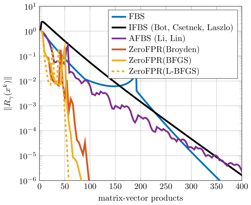
Figure 1. Nonconvex sparse approximation. Convergence of fixed-point residual in FBS and ZeroFPR, for different choices of the search directions, in the case $n=1500$, $\lambda=0.03$. Since ZeroFPR employs a linesearch, and therefore the complexity of each iteration is unknown a priori, we recorded the number of matrix-vector products by $A$ and $\trans{A}$ performed during the iterations, and display it on the horizontal axis.

$n$	$\lambda$	FBS	IFBS	AFBS	ZeroFPR(L-BFGS)
		avg/max (s)	avg/max (s)	avg/max (s)	avg/max (s)
500	0.10	0.141/0.405	0.159/0.449	0.135/0.221	0.037/0.088
	0.03	0.498/2.548	0.688/3.962	0.274/0.430	0.084/0.126
	0.01	1.305/5.445	1.721/4.942	0.570/1.157	0.152/0.560
1000	0.10	0.176/0.287	0.231/0.659	0.228/0.483	0.021/0.077
	0.03	0.576/2.756	0.645/4.165	0.382/0.841	0.091/0.275
	0.01	1.864/9.740	2.391/8.311	0.795/1.446	0.222/0.438
2000	0.10	0.291/0.599	0.392/0.719	0.393/0.640	0.025/0.055
	0.03	0.553/1.841	0.602/3.270	0.464/0.702	0.088/0.198
	0.01	2.108/10.934	2.439/8.010	0.979/1.411	0.271/0.464

Table 1. Nonconvex sparse approximation. Performance of FBS, IFBS, AFBS and ZeroFPR on problems with different values of $n$ and $\lambda$. The table shows average and maximum CPU time required to reach $\|R_{\gamma}(x^{k})\|\leq 10^{-6}$ in $100$ random experiments. Each algorithm was run on the same set of randomly generated problems, with $x^{0}=0$.

6.2. Dictionary learning

Given a collection of $m$ signals of dimension $n$, collected as columns in a matrix $Y\in\R^{n\times m}$, we seek for a sparse representation of each of them as combination of a set of $k$ vectors $\set{d_{1},\ldots,d_{k}}$, called dictionary atoms. To do so, we solve the following problem

(39) $$\minimize_{D,C}\ \tfrac{1}{2}\|Y-DC\|_{F}^{2}\quad\stt\leavevmode\nobreak\ \leavevmode\nobreak\ \begin{array}[t]{l@{~~}rl}\|d_{i}\|_{2}=1\hfil\leavevmode\nobreak\ \leavevmode\nobreak\ &i={}&1,\ldots,k,\\ \|c_{j}\|_{0}\leq N\hfil\leavevmode\nobreak\ \leavevmode\nobreak\ &j={}&1,\ldots,m,\\ \|c_{j}\|_{\infty}\leq T\hfil\leavevmode\nobreak\ \leavevmode\nobreak\ &j={}&1,\ldots,m,\end{array}$$

where $D=(d_{1},\ldots,d_{k})\in\R^{n\times k}$, $C=(c_{1},\ldots,c_{n})\in\R^{k\times m}$, $\|\cdot\|_{0}$ is the $\ell_{0}$ pseudo-norm, the number of nonzero coefficents, while $N\in\N$ and $T>0$ are parameters. This is similar to the problem considered in [1]. Here we bound the set of feasible points by means of the $\ell_{\infty}$-norm constraint: this has the effect of making the domain of problem (39) compact and $\nabla f$, as a consequence, Lipschitz continuous over the problem domain (cf. section 5.3). Furthermore, here we explicitly constrain the norm of the dictionary atoms: in fact, the objective value of (39) is unchanged if an atom $d_{i}$ is scaled by a factor, and the corresponding row of $C$ is scaled by the inverse factor.

Problem (39) takes the form (1) by letting $f(D,C)=\tfrac{1}{2}\|Y-DC\|^{2}_{F}$ and $g(D,C)=\delta_{S}(D,C)$, where $S{}={}\overbrace{S_{D}\times\ldots\times S_{D}}^{\text{$k$ times}}{}\times{}\overbrace{S_{C}\times\ldots\times S_{C}}^{\text{$m$ times}},$ with

$$S_{D}{}={}\set{d\in\R^{n}}[\|d\|_{2}=1],\quad S_{C}{}={}\set{\smash{c\in\R^{k}}}[\|c\|_{0}\leq N,\|c\|_{\infty}\leq T],$$

set $S$ is the product of Euclidean spheres and box-constrained $\ell_{0}$ level sets. Both $f$ and $g$ are nonconvex in this case. Projection onto $S_{D}$ is simply a matter of scaling, while that onto $S_{C}$ simply amounts to projecting the $N$ largest coefficients (in absolute value) onto the box $[-T,T]$ and setting to zero the remaining ones.

We have tested the proposed algorithm on a sequence of problems generated according to [1, §V.A]. We set $n=20$, $m=500$, $k=50$, therefore in this case the problem has $26000$ variables. A generating dictionary $D_{\mathrm{gen}}\in\R^{20\times 50}$ was selected randomly generated with normal entries, and each column was normalized to one. Then a random matrix $C_{\mathrm{gen}}\in\R^{50\times 500}$ was selected with $3$ normally distributed nonzero coefficient per column. Then we set $Y=C_{\mathrm{gen}}D_{\mathrm{gen}}+V$, where $V\in\R^{n\times m}$ is normally distributed with variance $10^{-2}$. We generated $50$ random problems according to this procedure, and applied the algorithms to problem (39) with $N=3$ and $T=10^{6}$. In this case IFBS is not applicable since the Lipschitz constant of $\nabla f$ over the problem domain is unknown, and an appropriate stepsize-selection rule is not provided for the algorithm in [14]. We compared FBS, AFBS and ZeroFPR, using the backtracking procedure discussed in Section 5.3 to adaptively adjust the stepsize $\gamma$. We used $(D^{0},C^{0})=(0,0)$ as initial iterate, while the algorithms were stopped as soon as $\|R_{\gamma}(x^{k})\|\leq 10^{-4}$. The results are shown in Figure 2: in most of the cases, ZeroFPR(L-BFGS) exhibited a speedup of a factor $5$-to-$100$ with respect to FBS, and $3$-to-$60$ with respect to AFBS, at reaching a critical point.

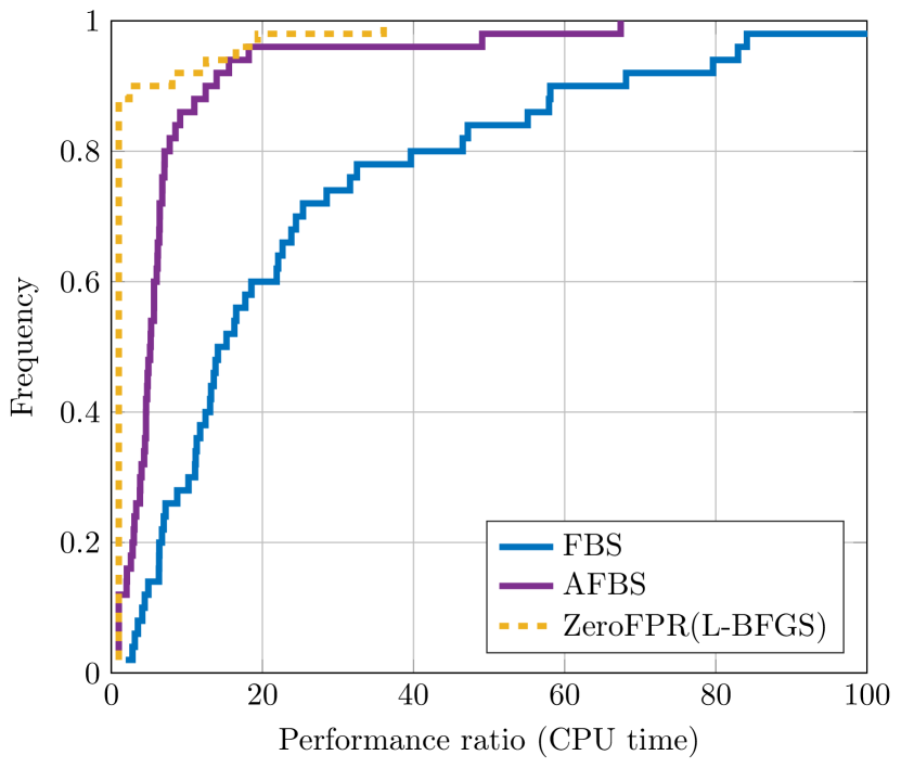
Figure 2. Dictionary learning. Performance profiles of FBS, AFBS and ZeroFPR(L-BFGS) when applied to $50$ randomly generated problems with $n=20$, $m=500$, $k=50$, $T=10^{6}$ and $N=3$. The algorithms are executed until tolerance $\|R_{\gamma}(x^{k})\|\leq 10^{-4}$ is reached. In the great majority of cases, ZeroFPR(L-BFGS) reaches a critical point significantly faster than FBS.

6.3. Matrix decomposition

We consider the problem of approximating a given matrix $A\in\R^{m\times n}$ as the sum of a low-rank and a sparse component, by solving

(40) $$\minimize_{X_{L},X_{S}\in\R^{m\times n}}\tfrac{1}{2}\|A-X_{L}-X_{S}\|_{F}^{2}+\lambda\|X_{S}\|_{0}\quad\stt\ \rank(X_{L})\leq r.$$

This problem has application, for example, in the analysis of video imagery, specifically the separation of the background (fixed over time) scenery from the foreground (moving) objects in a series of video frames. In this case, matrix $A$ contains $n$ video frames (columns), each consisting of $m$ pixels, and $X_{L}$, $X_{S}$ will respectively contain the background scenery and foreground objects identified in each frame. Therefore here $f(X_{L},X_{S})=\tfrac{1}{2}\|A-X_{L}-X_{S}\|_{F}^{2}$ and $L_{f}=2$, while $g(X_{L},X_{S})=\indicator_{\rank\leq r}(X_{L})+\lambda\|X_{S}\|_{0}$. The proximal mapping of $g$ is given by

$$\prox_{\gamma g}(X_{L},X_{S})=(\proj_{\rank\leq r}(X_{L}),\prox_{\gamma\lambda\|\cdot\|_{0}}(X_{S})).$$

Here, $\prox_{\gamma\lambda\|\cdot\|_{0}}$ is the hard-thresholding operation, defined componentwise as

$$\left[\prox_{\gamma\lambda\|\cdot\|_{0}}(X_{S})\right]_{ij}=\begin{cases}0&\quad\mbox{if\ }\bigl{(}X_{S}\bigr{)}_{ij}\leq\sqrt{2\gamma\lambda}\\ \bigl{(}X_{S}\bigr{)}_{ij}&\quad\mbox{otherwise}\end{cases}\quad i,j=1,\ldots,m.$$

The set of matrices of rank at most $r$ is nonconvex and closed, and the projection onto it is given by $\proj_{\rank\leq r}(X){}={}U_{r}\diag(\sigma_{1},\ldots,\sigma_{r})V_{r}^{T}$, where $\sigma_{1}\ldots\sigma_{r}$ are $r$ largest singular values of $X$, and $U_{r},V_{r}$ are the matrices of left and right singular vectors, respectively. Each computation of $\Pi_{\rank\leq r}$ requires a partial SVD which is, from the computational perspective, the most significantly expensive operation in this case.

We applied this technique to a sequence of $n=50$ frames coming from the ShoppingMall dataset. The footage consists of $m=320\times 256$ grayscale pixels frames, therefore the problem has $8192000$ variables in total. In problem (40) we used $r=1$ and $\lambda=3\cdot 10^{-3}$. The results are shown in Figures 3 and 4. Also in this case, the fast asymptotic convergence of ZeroFPR(L-BFGS) is apparent.

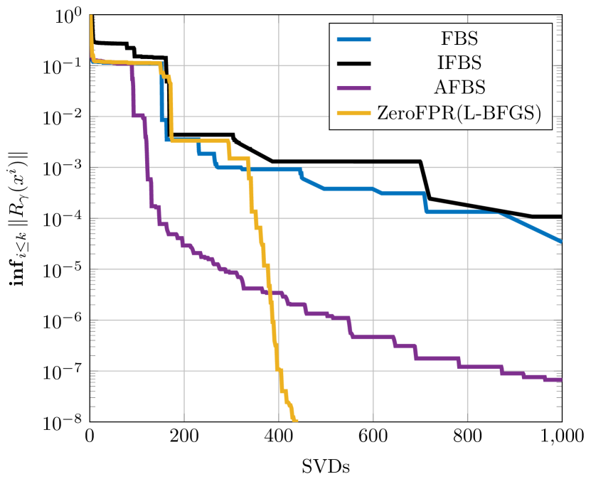
Figure 3. Matrix decomposition. Convergence of the fixed-point residual of ZeroFPR using L-BFGS directions compared to FBS and IFBS on the ShoppingMall dataset.

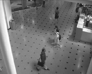
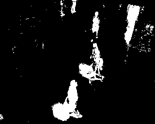
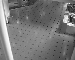
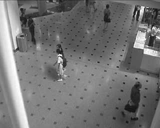
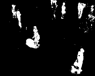
Figure 4. Matrix decomposition: separation of the background scenery from the foreground moving objects in the ShoppingMall dataset.

7. Conclusions

The forward-backward envelope is a valuable tool for deriving efficient algorithms tackling nonsmooth and nonconvex problems of the form $\varphi=f+g$, as it can be used as a merit function to devise globally convergent linesearch methods solving the system of nonlinear equations defining the stationary points of $\varphi$.

ZeroFPR implements this idea, and we proved that it globally converges to a stationary point under the assumption that $\varphi_{\gamma}$ has the Kurdyka-Łojasiewicz property. Furthermore, if the linesearch directions satisfy the Dennis-Moré condition (for example, if they are determined according to the Broyden method), the convergence rate at strong local minima is superlinear.

Numerical simulations with the proposed method on convex and nonconvex problems confirm our theoretical results. Using Broyden method, BFGS (in the case of small-scale problems) and L-BFGS (for large-scale problems) to compute directions in ZeroFPR greatly outperform FBS and its accelerated variant. It is our belief that the surprising efficacy of (L-)BFGS is due to the fact that, under the appropriate assumptions, the Jacobian of $R_{\gamma}$ at strong local minima is similar to a symmetric and positive definite matrix. Future investigation may better explain the effectiveness of symmetric update formulas in this framework.

Appendix A Proofs of Section 4

[Proof of Section 4.4]

• 1: It follows from [37, Thm.s 3.8 and 4.1] that $\prox_{\gamma g}$ is (strictly) differentiable at $x^{\star}-\gamma\nabla f(x^{\star})$ iff $g$ (strictly) satisfies item 2. Consequently, if $f$ is of class $C^{2}$ around $x^{\star}$ (and in particular strictly differentiable at $x^{\star}$ [44, Cor. 9.19]), $R_{\gamma}(x)=x-\FB x$ is (strictly) differentiable at $x^{\star}$ with Jacobian as in (17) due to the chain rule of differentiation (and the fact that strict differentiability is preserved by composition). For $\gamma^{\prime}\in(\gamma,\Gamma(x^{\star}))$ and $w\in\R^{n}$ we have

  $$\mathtight\twiceepi[-\nabla f(x^{\star})]{g}{x^{\star}}[w]{}={}\liminf_{\begin{subarray}{c}w^{\prime}\to\fillwidthof[l]{0^{+}}{w}\\ \fillwidthof[r]{w^{\prime}}{\tau}\to 0^{+}\end{subarray}}{\frac{g(x^{\star}+\tau w^{\prime}){}-{}g(x^{\star}){}+{}\tau\innprod{\nabla f(x^{\star})}{w}}{\nicefrac{{\tau^{2}}}{{2}}}}\leavevmode\nobreak\ {}\overrel[\geq]{\eqref{eq:ProxGrad'}}{}-\tfrac{1}{\gamma^{\prime}}\|w\|^{2}.$$

  The expression (15) of the second-order epi-derivative then implies $\innprod{Mw}{w}{}\geq{}-\frac{1}{\gamma^{\prime}}\|w\|^{2}$ for all $w\in\R^{n}$ (since $Mw=0$ for $w\in S^{\perp}$). Therefore, $\lambda_{\rm min}(M){}\geq{}-\nicefrac{{1}}{{\gamma^{\prime}}}{}>{}-\nicefrac{{1}}{{\gamma}}$, proving $I+\gamma M$ to be positive definite, and in particular invertible. We may now trace the proof of [45, Lem. 2.9] to infer that $JP_{\gamma}(x^{\star}){}={}\proj_{S}[I+\gamma M]^{-1}\proj_{S}$. Apparently, $JP_{\gamma}(x^{\star})$ is symmetric and positive semidefinite.

• 2: Since $Q_{\gamma}$ is (strictly) continuous at $x^{\star}$ and $R_{\gamma}$ is (strictly) differentiable at $x^{\star}$, from [45, Lem. 6.2] we have that $\nabla\varphi_{\gamma}=Q_{\gamma}R_{\gamma}$ is (strictly) differentiable at $x^{\star}$, and (17) follows by the chain rule.

• 3: A simple application of the chain rule proves (18); moreover, combined with (17) we obtain $\nabla^{2}\varphi_{\gamma}(x^{\star}){}={}\tfrac{1}{\gamma}\left[Q_{\gamma}(x^{\star}){}-{}Q_{\gamma}(x^{\star})P_{\gamma}(x^{\star})Q_{\gamma}(x^{\star})\right]$, and since both $Q_{\gamma}(x^{\star})$ and $P_{\gamma}(x^{\star})$ are symmetric, then so is $\nabla^{2}\varphi(x^{\star})$.

[Proof of Section 4.4]We will show that all conditions are equivalent to either one of the following

1. $\tinnprod{d}{(\nabla^{2}f(x^{\star})+M)d}>0$ $\forall d\in S$, where $M$ and $S$ are as in section 4.4;

2. $JR_{\gamma}(x^{\star})$ is similar to a symmetric and positive definite matrix.

• 4.4 $\Leftrightarrow$ 4.4: trivial, since $\nabla^{2}\varphi_{\gamma}(x^{\star})$ exists as shown in item 3.

• 4.4 $\Leftrightarrow$ thm:StrongMinimality(f): follows from [44, Thm. 13.24(c)], since

  $$\twiceepi[0]{\varphi}{x^{\star}}[d]{}={}\tinnprod{d}{\nabla^{2}f(x^{\star})d}{}+{}\twiceepi[-\nabla f(x^{\star})]{g}{x^{\star}}[d]{}={}\tinnprod{d}{(\nabla^{2}f(x^{\star})+M)d}+\delta_{S}(d).$$

• 4.4 $\Leftrightarrow$ 4.4: if $\nabla^{2}\varphi_{\gamma}(x^{\star})\succ 0$, then $x^{\star}$ is a (strong) local minimum for $\varphi_{\gamma}$ and, due to (18), necessarily $JR_{\gamma}(x^{\star})$ is invertible. Conversely, if $x^{\star}$ is a local minimum for $\varphi_{\gamma}$, then $\nabla^{2}\varphi_{\gamma}(x^{\star})\succeq 0$. If, additionally, $JR_{\gamma}(x^{\star})$ is invertible, then due to (18) $\nabla^{2}\varphi_{\gamma}(x^{\star})$ is also invertible, and therefore positive definite.

• 4.4 $\Leftrightarrow$ thm:StrongMinimality(g): by comparing (17) and (18) we observe that $JR_{\gamma}(x^{\star})$ is similar to the (symmetric) matrix $Q_{\gamma}(x^{\star})^{-\nicefrac{{1}}{{2}}}\nabla^{2}\varphi_{\gamma}(x^{\star})Q_{\gamma}(x^{\star})^{-\nicefrac{{1}}{{2}}}$, which is positive definite iff $\nabla^{2}\varphi_{\gamma}(x^{\star})$ is.

• thm:StrongMinimality(f) $\Leftrightarrow$ thm:StrongMinimality(g): the proof is the same as that of [45, Thm. 2.11(b)$\Leftrightarrow$(c)].

• 4.4 $\Rightarrow$ thm:StrongMinimality(g): with similar reasonings as in the proof of the implications “4.4 $\Leftrightarrow$ thm:StrongMinimality(f) $\Leftrightarrow$ thm:StrongMinimality(g)”, we conclude that local minimality of $x^{\star}$ for $\varphi$ entails $JR_{\gamma}(x^{\star})$ being similar to a symmetric and positive semidefinite matrix. Therefore, if $JR_{\gamma}(x^{\star})$ is nonsingular, then it is similar to a symmetric and positive definite matrix.

• 4.4 $\Rightarrow$ 4.4: trivial, since $\varphi_{\gamma}\leq\varphi$ and $\varphi_{\gamma}(x^{\star})=\varphi(x^{\star})$ (cf. items 1 and 1).

Appendix B Additional results for Section 5

Consider the iterates generated by ZeroFPR and suppose that the directions $\seq{d^{k}}$ are selected so as to satisfy (31). Then,

1. $\|x^{k+1}-x^{k}\|{}\leq{}(\gamma+D)\|r^{k}\|$

2. $\|\bar{x}^{k+1}-\bar{x}^{k}\|{}\leq{}\gamma\|r^{k+1}\|{}+{}(2\gamma+D)\|r^{k}\|$

3. in particular, $\|x^{k+1}-x^{k}\|$ and $\|\bar{x}^{k+1}-\bar{x}^{k}\|$ converge to 0.

For all $k$ we have

$$\|x^{k+1}-x^{k}\|{}={}\|\bar{x}^{k}+\tau_{k}d^{k}-x^{k}\|{}={}\|\tau_{k}d^{k}-\gamma r^{k}\|{}\leq{}\gamma\|r^{k}\|{}+{}\tau_{k}\|d^{k}\|{}\leq{}(\gamma+D)\|r^{k}\|$$

where in the last inequality we used the fact that $\tau_{k}\in(0,1]$. This proves 1, and 2 trivially follows by the triangular inequality $\|\bar{x}^{k+1}-\bar{x}^{k}\|{}\leq{}\|x^{k+1}-x^{k}\|{}+{}\gamma\|r^{k+1}\|{}+{}\gamma\|r^{k}\|$. Using this, 3 follows from item 1.

Consider the iterates generated by ZeroFPR. Suppose that (31) is satisfied and that the sequence $\seq{x^{k}}$ is bounded. Then, $\omega(x^{k})=\omega(\bar{x}^{k})$ are nonempty compact and connected sets over which $\varphi$ and $\varphi_{\gamma}$ are constant and coincide. Moreover,

(41) $$\lim_{k\to\infty}{\dist(x^{k},\omega(x^{k}))}{}={}\lim_{k\to\infty}{\dist(\bar{x}^{k},\omega(x^{k}))}{}={}0.$$

The sets of cluster points are nonempty because of boundedness of the sequences; in turn, connectedness and compactness as well as (41) are shown in [12, Rem. 5], which applies since $\|x^{k+1}-x^{k}\|$ and $\|\bar{x}^{k+1}-\bar{x}^{k}\|$ converge to $0$ (cf. item 3). Moreover, since $\seq{\varphi_{\gamma}(x^{k})}$ converges to some value $\varphi_{\star}\in\R$ and $\omega(x^{k})=\omega(\bar{x}^{k})\subseteq\fix T_{\gamma}$ as shown in section 5.4, it follows Item 1 that $\varphi$ and $\varphi_{\gamma}$ coincide on $\omega(x^{k})$ (and equal $\varphi_{\star}$).

Suppose that Section 4.4 is satisfied at a strong local minimum $x^{\star}$ of $\varphi$. Then, for any $\gamma\in(0,\nicefrac{{1}}{{L_{f}}})$ the FBE $\varphi_{\gamma}$ possesses the KL property at $x^{\star}$, and the desingularizing function $\psi$ can be taken of the form $\psi(s){}={}\rho s^{\nicefrac{{1}}{{2}}}$ for some $\rho>0$. From section 4.4 it follows that $x^{\star}$ is a strong local minimum for $\varphi_{\gamma}$ at which $\varphi_{\gamma}$ is twice differentiable with $H_{\star}\coloneqq\nabla^{2}\varphi_{\gamma}(x^{\star})\succ 0$. Let $\lambda{}\coloneqq{}\lambda_{\rm min}(H_{\star})$ and $\Lambda{}\coloneqq{}\lambda_{\rm max}(H_{\star})$. Since $\nabla\varphi_{\gamma}(x^{\star})=0$, from a second-order expansion of $\varphi_{\gamma}$ and a first-order expansion of $\nabla\varphi_{\gamma}$ we obtain that there exists a neighborhood $U_{x^{\star}}$ of $x^{\star}$ such that, for all $x\in U_{x^{\star}}$, $\varphi_{\gamma}(x)-\varphi_{\gamma}(x^{\star}){}\leq{}\tfrac{\Lambda}{4}\|x-x^{\star}\|^{2}$ and $\|\nabla\varphi_{\gamma}(x)\|{}\geq{}\tfrac{\lambda}{2}\|x-x^{\star}\|$, and in particular $\psi^{\prime}\left(\varphi_{\gamma}(x)-\varphi_{\gamma}(x^{\star})\right)\|\nabla\varphi_{\gamma}(x)\|{}={}\tfrac{\rho}{2\sqrt{\varphi_{\gamma}(x)-\varphi_{\gamma}(x^{\star})}}\|\nabla\varphi_{\gamma}(x)\|{}\geq{}\tfrac{\rho\lambda}{2\sqrt{\Lambda}}$. Letting $\rho{}={}\frac{2\sqrt{\Lambda}}{\lambda}$ we obtain that $\psi$ is a KL function for $\varphi_{\gamma}$ at $x^{\star}$.

References

- [1] Michal Aharon, Michael Elad, and Alfred Bruckstein. K-SVD: An algorithm for designing overcomplete dictionaries for sparse representation. IEEE Transactions on signal processing, 54(11):4311–4322, 2006.
- [2] F. J. Aragón Artacho, A. Belyakov, A. L. Dontchev, and M. López. Local convergence of quasi-Newton methods under metric regularity. Computational Optimization and Applications, 58(1):225–247, 2014.
- [3] Hedy Attouch and Jérôme Bolte. On the convergence of the proximal algorithm for nonsmooth functions involving analytic features. Mathematical Programming, 116(1-2):5–16, 2009.
- [4] Hédy Attouch, Jérôme Bolte, Patrick Redont, and Antoine Soubeyran. Proximal alternating minimization and projection methods for nonconvex problems: An approach based on the Kurdyka-łojasiewicz inequality. Mathematics of Operations Research, 35(2):438–457, 2010.
- [5] Hedy Attouch, Jérôme Bolte, and Benar Fux Svaiter. Convergence of descent methods for semi-algebraic and tame problems: proximal algorithms, forward–backward splitting, and regularized gauss–seidel methods. Mathematical Programming, 137(1):91–129, 2013.
- [6] Hedy Attouch and Juan Peypouquet. The rate of convergence of Nesterov’s accelerated forward-backward method is actually faster than . SIAM Journal on Optimization, 26(3):1824–1834, 2016.
- [7] Amir Beck and Nadav Hallak. On the minimization over sparse symmetric sets: Projections, optimality conditions, and algorithms. Math. Oper. Res., 41(1):196–223, 2016.
- [8] Amir Beck and Marc Teboulle. A Fast Iterative Shrinkage-Thresholding Algorithm for Linear Inverse Problems. SIAM Journal on Imaging Sciences, 2(1):183–202, 2009.
- [9] Dimitri P. Bertsekas. Nonlinear Programming. Athena Scientific, 1995.
- [10] J. Bochnak, M. Coste, and M-F. Roy. Real Algebraic Geometry. Springer, 1998.
- [11] Jérôme Bolte, Aris Daniilidis, and Adrian Lewis. The Łojasiewicz inequality for nonsmooth subanalytic functions with applications to subgradient dynamical systems. SIAM Journal on Optimization, 17(4):1205–1223, 2007.
- [12] Jérôme Bolte, Shoham Sabach, and Marc Teboulle. Proximal alternating linearized minimization for nonconvex and nonsmooth problems. Mathematical Programming, 146(1-2):459–494, 2014.
- [13] Jérôme Bolte and Edouard Pauwels. Majorization-minimization procedures and convergence of SQP methods for semi-algebraic and tame programs. Mathematics of Operations Research, 41(2):442–465, 2016.
- [14] Radu Ioan Boţ, Ernö Robert Csetnek, and Szilárd Csaba László. An inertial forward–backward algorithm for the minimization of the sum of two nonconvex functions. EURO Journal on Computational Optimization, 4(1):3–25, 2016.
- [15] Charles G. Broyden. A class of methods for solving nonlinear simultaneous equations. Mathematics of Computation, 19(92):577–593, 1965.
- [16] Richard H. Byrd and Jorge Nocedal. A tool for the analysis of quasi-Newton methods with application to unconstrained minimization. SIAM J. Numer. Anal., 26(3):727–739, June 1989.
- [17] Aris Daniilidis, Warren Hare, and Jérôme Malick. Geometrical interpretation of the predictor-corrector type algorithms in structured optimization problems. Optimization, 55(5-6):481–503, 2006.
- [18] Ingrid Daubechies, Ronald DeVore, Massimo Fornasier, and C. Sinan Güntürk. Iteratively reweighted least squares minimization for sparse recovery. Communications on Pure and Applied Mathematics, 63(1):1–38, 2010.
- [19] John E. Dennis and Jorge J. Moré. A characterization of superlinear convergence and its application to quasi-Newton methods. Mathematics of computation, 28(126):549–560, 1974.
- [20] Asen Dontchev. Generalizations of the dennis–moré theorem. SIAM Journal on Optimization, 22(3):821–830, 2012.
- [21] Pierre Frankel, Guillaume Garrigos, and Juan Peypouquet. Splitting methods with variable metric for kurdyka–łojasiewicz functions and general convergence rates. Journal of Optimization Theory and Applications, 165(3):874–900, 2015.
- [22] Chi-Ming Ip and Jerzy Kyparisis. Local convergence of quasi-Newton methods for B-differentiable equations. Mathematical Programming, 56(1-3):71–89, 1992.
- [23] A. Kaplan and R. Tichatschke. Proximal point methods and nonconvex optimization. Journal of Global Optimization, 13(4):389–406, 1998.
- [24] Krzysztof Kurdyka. On gradients of functions definable in o-minimal structures. Annales de l’institut Fourier, 48(3):769–783, 1998.
- [25] A. S. Lewis. Active sets, nonsmoothness, and sensitivity. SIAM Journal on Optimization, 13(3):702–725, 2002.
- [26] Huan Li and Zhouchen Lin. Accelerated proximal gradient methods for nonconvex programming. In Advances in neural information processing systems, pages 379–387, 2015.
- [27] Dong C. Liu and Jorge Nocedal. On the limited memory BFGS method for large scale optimization. Mathematical Programming, 45(1-3):503–528, 1989.
- [28] Tianxiang Liu and Ting Kei Pong. Further properties of the forward–backward envelope with applications to difference-of-convex programming. Computational Optimization and Applications, pages 1–32, 2017.
- [29] Stanislaw Łojasiewicz. Une propriété topologique des sous-ensembles analytiques réels. Les équations aux dérivées partielles, pages 87–89, 1963.
- [30] Stanislaw Łojasiewicz. Sur la géométrie semi- et sous- analytique. Annales de l’institut Fourier, 43(5):1575–1595, 1993.
- [31] B. Martinet. Brève communication. Régularisation d’inéquations variationnelles par approximations successives. ESAIM: Modélisation Mathématique et Analyse Numérique, 4(R3):154–158, 1970.
- [32] Yuri Nesterov. Gradient Methods for Minimizing Composite Functions. Mathematical Programming, 140(1):125–161, 2013.
- [33] Jorge Nocedal. Updating quasi-Newton matrices with limited storage. Mathematics of computation, 35(151):773–782, 1980.
- [34] Jorge Nocedal and Stephen Wright. Numerical Optimization. Springer, New York, 2nd edition edition, August 2006.
- [35] Peter Ochs, Yunjin Chen, Thomas Brox, and Thomas Pock. iPiano: Inertial proximal algorithm for nonconvex optimization. SIAM Journal on Imaging Sciences, 7(2):1388–1419, 2014.
- [36] Panagiotis Patrinos and Alberto Bemporad. Proximal Newton methods for convex composite optimization. In IEEE Conference on Decision and Control, pages 2358–2363, 2013.
- [37] RA Poliquin and RT Rockafellar. Generalized Hessian properties of regularized nonsmooth functions. SIAM Journal on Optimization, 6(4):1121–1137, 1996.
- [38] René A. Poliquin and R. Tyrrell Rockafellar. Amenable functions in optimization. Nonsmooth optimization: methods and applications, pages 338–353, 1992.
- [39] René A Poliquin and R. Tyrrell Rockafellar. Second-order nonsmooth analysis in nonlinear programming. Recent advances in nonsmooth optimization, pages 322–349, 1995.
- [40] René A Poliquin and R. Tyrrell Rockafellar. Prox-regular functions in variational analysis. Transactions of the American Mathematical Society, 348(5):1805–1838, 1996.
- [41] M. Powell. A hybrid method for nonlinear equations. Numerical Methods for Nonlinear Algebraic Equations, pages 87–144, 1970.
- [42] R. Tyrrell Rockafellar. First- and second-order epi-differentiability in nonlinear programming. Transactions of the American Mathematical Society, 307(1):75–108, 1988.
- [43] R. Tyrrell Rockafellar. Second-order optimality conditions in nonlinear programming obtained by way of epi-derivatives. Mathematics of Operations Research, 14(3):462–484, 1989.
- [44] R. Tyrrell Rockafellar and Roger J.B. Wets. Variational analysis, volume 317. Springer, 2011.
- [45] Lorenzo Stella, Andreas Themelis, and Panagiotis Patrinos. Forward–backward quasi-Newton methods for nonsmooth optimization problems. Computational Optimization and Applications, pages 1–45, 2017.
- [46] Zongben Xu, Xiangyu Chang, Fengmin Xu, and Hai Zhang. regularization: a thresholding representation theory and a fast solver. IEEE Transactions on neural networks and learning systems, 23(7):1013–1027, 2012.
- [47] Hongchao Zhang and William W. Hager. A nonmonotone line search technique and its application to unconstrained optimization. SIAM Journal on Optimization, 14(4):1043–1056, 2004.