An Empirical Comparison of Sampling Quality Metrics:
A Case Study for Bayesian Nonnegative Matrix Factorization

1 Introduction

Bayesian approaches to machine learning begin by positing that the data $X$ can be explained by some probablistic model $p(X|\theta)$, where $\theta$ is a set of parameters. Rather than finding a point estimate for $\theta$ that maximizes the likelihood $p(X|\theta)$, Bayesian approaches place a a prior distribution over the parameters $p(\theta)$ and compute the posterior $p(\theta|X)$. The posterior $p(\theta|X)$ captures uncertainty in the parameters $\theta$.

For most models, the posterior $p(\theta|X)$ does not have an analytic form. In this situation, a popular approach is to approximate the posterior $p(\theta|X)$ through a set of samples $\{\theta_{1},..,\theta_{N}\}$. Approaches for generating these samples include importance and rejection sampling Liu (1996), sequential Monte Carlo Halton (1962), and Markov Chain Monte Carlo Gilks (2005).

In this work, we empirically explore the question: how can we assess the quality of these samples? We assume that the samples are provided by some valid Monte Carlo procedure, so we are guaranteed that the collection of samples will asymptotically approximate the true posterior $p(\theta|X)$. Most current evaluation approaches focus on two questions: (1) Has the chain mixed, that is, is it sampling from the posterior $p(\theta|X)$? and (2) How independent are the samples (as MCMC procedures produce correlated samples)? Focusing on the case of Bayesian nonnegative matrix factorization, we empirically evaluate standard metrics of sampler quality as well as propose new metrics to capture aspects that these measures fail to expose. The aspect of sampling that is of particular interest to us is the ability (or inability) of sampling methods to move between multiple optima in NMF problems. As a proxy, we propose and study a number of metrics that might quantify the diversity of a set of NMF factorizations obtained by a sampler through quantifying the coverage of the posterior distribution. We compare the performance of a number of standard sampling methods for NMF in terms of these new metrics.

2 Background

2.1 Current Measures of Sampling Quality

Measures of Mixing.

While it is practically impossible to assess whether a chain has mixed, some popular approaches include sample paths, cumulative sums, autocorrelation plots, batch means, AR and spectral analysis estimators Johnson (1996); Cowles and Carlin (1996); Flegal et al. (2010).

Measures of Sample Independence.

Most current approaches to measuring sampling quality focus on measuring the independence the samples from the chain. Since sample independence is hard to assess, most measures focus on correlation between samples. These include: effective sample size, autocorrelation plots, cross-correlation, integrated autocorrelation time, Hairiness Index Cowles and Carlin (1996); Brooks (1998).

Other Measures

In the theoretical literature, other popular measures include cover time, hitting time, etc Aldous and Fill ; Lee et al. (2015). However, these are impractical in large scenarios or when the modes of the posterior distribution are unknown.

2.2 Bayesian Non-negative Matrix Factorization

In the case study below, we will evaluate several metrics of sample quality in the context of Bayesian nonnegative matrix factorization. We choose this example because it is one of the simplest and popular data exploration techiniques—NMF has been used to in wide-ranging applications ranging from understanding protein-protein interactions Greene et al. (2008), finding topics in large text corpora Roberts et al. (2016), and discovering molecular pathways from genomic samples Brunet et al. (2004)—with a myriad of efficient algorithms for solving it Paisley et al. (2015); Schmidt et al. (2009); Moussaoui et al. (2006); Lin (2007); Lee and Seung (2001); Recht et al. (2012). However, NMF still suffers from non-identifiability: even in the exact case, there can be multiple solutions. Thus, it serves a good test case for measuring how well current Bayesian approaches can describe this uncertainty.

Nonnegative Matrix Factorization and Identifiability

Given an $D\times N$ nonnegative matrix $X$ and desired rank $R$, the nonnegative matrix factorization (NMF) problem involves finding an $R\times N$ nonnegative weight matrix $W$, and an $D\times R$ nonnegative basis matrix $A$, such that $X\approx AW$. The ease of interpreting the weights $W$ and bases $A$ (due to the nonnegativity constraints), and the myriad of efficient algorithms for solving NMF Paisley et al. (2015); Schmidt et al. (2009); Moussaoui et al. (2006); Lin (2007); Lee and Seung (2001); Recht et al. (2012), has made NMF—and related models, such as topic models—a popular approach to data exploration in many fields. NMF has been used to understand protein-protein interactions Greene et al. (2008), find topics in large text corpora Roberts et al. (2016), and discover molecular pathways from genomic samples Brunet et al. (2004).

However, in many cases NMF is not identifiable: there may be very different pairs $(A,W)$ and $(A^{\prime},W^{\prime})$ that might explain the data $X$ (perhaps almost) as well. In the following, we briefly recall some relevant terminology and properties of NMF related to the notion of identifiability.

If $X=AW$, we call the pair $(A,W)$ an exact NMF; the minimum rank $R$ such that $X$ admits an exact NMF is called the nonnegative rank of $X$ and is denoted $\mathrm{rank}_{+}(X)$. A nonnegative matrix factorization, $X=AW$, can be considered trivially non-unique. Given any permutation matrix $P$ and diagonal matrix $D$ with positive entries, we obtain an alternate factorization of $X$, namely, $X=(AP^{\top}D^{-1})(DPW)$. Since the factorization ($AP^{\top}D^{-1}$, $DPW$) differs from ($A$, $W$) by scaling and relabeling of the column vectors in $A$, we consider them equivalent. Thus, we call an NMF unique if all solutions can be represented as $AQQ^{-1}W$, where $Q$ is a monomial matrix (i.e. a product of some $P$ and some $D$).

Awareness and concerns of non-identifabiltity has been gaining attention among practitioners. For example, Greene et al. (2008) use ensembles of NMF solutions to model chemical interactions, while Roberts et al. (2016) conduct a detailed empirical study of multiple optima in the context of extracting topics from large corpora. These approaches use random restarts to find multiple optima.

Bayesian Nonnegative Matrix Factorization

Bayesian NMF approaches Schmidt et al. (2009); Moussaoui et al. (2006) promise to characterize parameter uncertainty in a principled manner by solving for the posterior $p(A,W|X)$ given priors $p(A)$ and $p(W)$. Having such a representation of uncertainty in the bases and weights can further assist with the proper interpretation of the factors: we may place more confidence in subspace directions with low uncertainty, while subspace directions with more uncertainty may require further exploration. Unfortunately, in practice, the uncertainty estimates are often of limited use: sampling-based approaches Schmidt et al. (2009); Moussaoui et al. (2006) rarely switch between multiple modes.

In this case study, we will use the generative model of Schmidt et. al. in Schmidt et al. (2009). In this case, we place exponential priors $p(A)$ and $p(W)$ on $A$ and $W$ and choose a Gaussian likelihood. Thus, the elements of $W$, $A$ are sampled from a rectified normal distributions $\mathcal{R}(x;\mu,\sigma^{2},\lambda)$, which is proportional to the product of a Gaussian and an exponential $\mathcal{N}(x;\mu,\sigma^{2})\text{Exp}(x;\lambda)$. The full condition for the entries in $A|Q$ is given by

$$p(A_{d,r} |X,A_{\backslash(d,r)},W,\sigma^{2})=\mathcal{R}(A_{d,r};\mu_{A_{d,r}},\sigma^{2}_{A_{d,r}},\lambda_{A_{d,r}})$$

$$\mu_{A_{d,r}} =\frac{\sum_{n}(X_{d,n}-\sum_{r^{\prime}\neq r}A_{d,r^{\prime}}W_{r^{\prime},n})}{\sum_{n}W_{r,n}^{2}},\quad\sigma^{2}_{A_{d,r}}=\frac{\sigma^{2}}{\sum_{n}W_{r,n}^{2}}$$

with a symmetric update for $W$.

3 Additional Measures of Sample Quality: Notions of Coverage

The measures in Section 2.1 largely focus on the independence of samples. However, even in relatively simple models, such as Bayesian NMF, it is possible for a chain to mix quickly within a single mode and never reach an alternate mode or region. What is often missing in our discussion of practical MCMC approaches is a notion of coverage: In addition to moving in “independent” ways, how much of the posterior space does a finite-length chain explore? (Obviously given infinite time, every correct MCMC procedure will find all the modes.) In this section, we describe several easy-to-compute and principled measures of coverage that can be applied to any set of samples, whether or not they come from a Markov Chain.

3.1 Measures of Similarity

To quantify the “diversity” of a set of samples , we first need a notion of distance or similarity between a pair of samples. Below, we describe two matrix similarity measures, which can be meaningfully interpreted in the context of Bayesian NMF. Later, we show that the choice of one similarity measure may be more appropriate than another depending on the NMF model and the application.

Recall from Section 2.2 that we consider two basis matrices $A$ and $A^{\prime}$ to be equivalent (defining the same factorization of $X$) when $A^{\prime}=AQ$ for some monomial matrix $Q$. Thus, we need to ensure that each similarity measure we construct is defined on equivalence classes of matrices; that is, the disimilarity of two matrices in the same class should be zero. To do this, we scale each column in our matrices to be unit in some norm and we use permutation invariant representations of matrices (e.g. matrices as unordered collections of column vectors).

Minimum Matching Distance

For a fixed metric $m$ on $\mathbb{R}^{D}$, the minimum matching distance is a metric supported on sets of vectors in $\mathbb{R}^{D}$ Walters (2011). Given two subsets of $\mathbb{R}^{D}$, $A=\{A_{1},\ldots,A_{R}\}$ and $A^{\prime}=\{A^{\prime}_{1},\ldots,A^{\prime}_{R}\}$, their minimum matching distance is defined as

$$d_{\mathrm{MM}}(A,A^{\prime})=\min_{\sigma\in S_{R}}\sum_{r=1}^{R}d(A_{\sigma(r)},A^{\prime}_{\sigma(r)})$$ (1)

where $S_{R}$ is the set of of permutations of the index set $\{1,\ldots,R\}$. Intuitively, the minimum matching distance measures the total distance of the corresponding vectors of $A$ in $A^{\prime}$, minimized over all bipartite matchings of the vectors. The minimum matching distance can be efficiently computed using the Kuhn-Munkres algorithm Kriegel et al. (2003); Brecheisen et al. .

$\ell_{1}$ Matching

We fix the metric as $\ell_{1}$. Given $A,A^{\prime}\in\mathbb{R}^{R\times D}$ each with columns that are unit $\ell_{1}$-norm, we can compute their minimum matching distance as:

$$d_{\mathrm{MM}_{\ell_{1}}}(A,A^{\prime})=\min_{P\in\mathcal{P}}{\|AP-A^{\prime}\|_{1}},$$ (2)

where $\mathcal{P}$ is the set of $R\times R$ permutation matrices. Note that since the columns of $A$ and $A^{\prime}$ are unit $\ell_{1}$-norm, $d_{\mathrm{MM}_{\ell_{1}}}(A,A^{\prime})$ is bounded between $0$ and $R$.

The $\ell_{1}$ minimum matching distance measurement is closely related to the total variation distance for comparing discrete probability distributions. In the case of topic modeling, each column of $A$ or $A^{\prime}$ corresponds to a “topic”, which can be interpreted as a probability distribution over words in a dictionary. The $\ell_{1}$ minimum matching distance is (up to scale) the total variation distance after pairwise matching topics in $A$ and $A^{\prime}$ based on similarity.

Maximum Angle Similarity

Masood et al Masood and Doshi-Velez (2016) defines an angle-based similarity measurement that aims to capture the permutation ambiguity as well as the essence of a diverse factorization. Given $A,A^{\prime}\in\mathbb{R}^{R\times D}$, let $\widehat{\sigma}$ be a permutation of the columns of $A^{\prime}$ that minimizes the average angle between corresponding columns,

$$\widehat{\sigma}=\arg\min_{\sigma\in S_{R}}\frac{1}{R}\sum_{r\in R}\cos^{-1}\left(\frac{A_{r}\cdot A^{\prime}_{\sigma(r)}}{\|A_{r}\|\|A^{\prime}_{\sigma(r)}\|}\right)$$ (3)

The maximum angle similarity of $A$ and $A^{\prime}$ is defined largest angle between corresponding columns, under the permutation $\widehat{\sigma}$,

$$d_{\text{Angle}}(A,A^{\prime})=\max_{r\in R}\;\cos^{-1}\left(\frac{A_{r}\cdot A^{\prime}_{\widehat{\sigma}(r)}}{\|A_{r}\|\|A^{\prime}_{\widehat{\sigma}(r)}\|}\right)$$

As the entries in $A$ and $A^{\prime}$ are non-negative, the above dot product must always be non-negative. Thus, $d_{\text{Angle}}(A,A^{\prime})$ is bounded between $0$ and $\pi/2$.

Since the maximum angle similarity is measurement of orientation, we can apply the same measurement to basis elements of different dimensions and interpret the results in a similar manner. By focusing only on measuring the maximum angle, we allow for an extreme case where two factorizations only differ by one basis element. This may well be the case in some scenario so we incorporate it as a feature of this distance measurement.

In addition, by considering the maximum angle, our similarity measure gains a certain degree of robustness to column perturbations. For example, a similarity measurement based on the sum of angles between basis elements would not be successful in differentiating between a case where one basis element is significantly different versus if all basis elements were just perturbed a little bit. We want our understanding of diversity to be robust to perturbation of existing basis columns.

Notes and Observations about similarity in NMF basis factors:

Consider as a baseline, measuring the similarity as the Frobenius error of the difference i.e. $d_{F}(A,A^{\prime})=\|A-A^{\prime}\|_{F}$. Figure 1 shows two pairs of matrices $(A_{1},A_{2})$ and $(A_{1},A_{3})$ that have the same difference in the naive Frobenius sense ($d_{F}$ = 0.122) but different maximum angle and $l_{1}$-minimum matching similarity scores. From figure 1 it is also clear that the $(A_{1},A_{3})$ pair is the more dissimilar. This example illustrate the fact that these measures of similarity indeed capture the sense of diversity in solutions that is of interest to us.

Finally, we point out that the permutation computed in the minimum matching distance, which minimizing the total distance between matrices, is not necessarily the same as the permutation, which minimizes the average angle between corresponding columns. In practice, this means that permutations used to compute the minimum matching distance cannot be used to compute the maximum angle distance (and vice versa). It also raises an interesting question about what is means in empirical work to ‘correct’ for the permutation ambiguity since we’ve observed that this correction is metric-dependent.

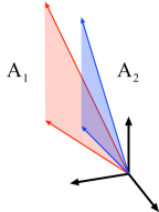
(a) $d_{\mathrm{MM}_{\ell_{1}}}(A_{1},A_{2})=0.137$, $d_{\text{Angle}}(A_{1},A_{2})=6.38$

(b) $d_{\mathrm{MM}_{\ell_{1}}}(A_{1},A_{3})=0.400$, $d_{\text{Angle}}(A_{1},A_{3})=20.44$

Figure 1: Comparison of max angle and $\ell_{1}$-min match measures when $\|A_{1}-A_{2}\|_{F}=\|A_{1}-A_{3}\|_{F}$.

3.2 Measures of Coverage

Given a set, $S$, of samples from some parameter space explore by a sampler, and given a similarity measure $m$ for pairs of samples, we introduce three measurement of the diversity of the samples contained in $S$.

Maximum Pairwise Distance

We define a notion of diversity for a set $S$ based on the “diameter” of $S$, that is, we compute the maximum distance between pairs of points points in $S$. The maximum pairwise distance of $S$ is defined as

$$\mathrm{MaxDist}(S)=\max_{A,A^{\prime}\in S}d(A,A).$$ (4)

Mean Pairwise Distance

We can alternatively quantify the diversity of $S$ by approximating the “density” of points in $S$. Motivate by this intuition, we define the mean pairwise distance of $S$ as

$$\mathrm{MeanDist}(S)=\frac{1}{|A|^{2}}\sum_{A,A^{\prime}\in S}d(A,A).$$ (5)

Covering Number

We quantify the amount of the parameter space explored by the sampler, by approximating a notion of“volume” for a set of samples $S$. For each $\epsilon>0$, we define the minimum covering number of $S$, denoted $C_{\epsilon}(S)$, as the cardinality of the smallest subset $S^{\prime}\subset S$ such that $\underset{s\in S^{\prime}}{\bigcup}B(s,\epsilon)$ covers $S$, where $B(s,\epsilon)$ is the $\epsilon$ ball centered at $s$ with respect to some metric or similarity measure. Our minimum covering number can stated in terms of the covering number of graphs of the $\epsilon$-neighbor graph of the points in $S$. We note that the covering number is a frequently studied property of graphs in literature Abbott and Liu (1979); Chepoi et al. (2007).

Clearly, $C_{\epsilon}(S)$ depends on the choice of $\epsilon$. When $\epsilon=0$, the minimum covering number is equal to the cardinality of $S$; for sufficiently large $\epsilon$, the minimum covering number is 1, since an $\epsilon$-ball centered at any element will contain the entire set $S$. It is also straightforward to see that $C_{\epsilon}$ is a monotone increasing as a function of $\epsilon$.

Generally speaking, for a fixed $\epsilon$, the larger the minimum covering number, the more of the parameter space covered by the sampler. However, cases may arise, for $\epsilon_{1}<\epsilon_{2}$ and sets $S_{1}$, $S_{2}$, where $C_{\epsilon_{1}}(S_{1})>C_{\epsilon_{1}}(S_{2})$ but $C_{\epsilon_{2}}(S_{1})<C_{\epsilon_{2}}(S_{2})$. In Figure 2 and Figure 3, we see samples $S_{1}$, $S_{2}$ from a mixture of two Gaussians, where $S_{1}$ is concentrated in one mode and $S_{2}$ is distributed amongst both modes. The latter is demonstrated by the fact that $C_{\epsilon_{2}}(S_{2})>C_{\epsilon_{2}}(S_{1})$ for sufficiently large choices of $\epsilon$.

To avoid arbitrariness in selecting a single value for $\epsilon$, we compute the minimum covering number for a range for values between $\epsilon=0$ and $\epsilon=t$, for $t$ is sufficiently large that each $\epsilon$-ball covers $S$. We interpret covering numbers which “persists” for significant intervals of $\epsilon$ to be revealing the diversity of the sample set and covering numbers which appear for small intervals of $\epsilon$ to be negligible (due to small variations in the set). The motivation for our interpretation is based in the body of work on persistent topology Edelsbrunner and Harer (2008); Carlsson (2009); Ghrist (2008), in which topological features of manifolds are deduced from an approximation given by a set of sample points by interpreting the features which persist in the reconstruction across a number of resolutions.

We call the collection of the covering numbers which persists for large intervals of $\epsilon$, or, in a slight abuse of language, the collection of covering numbers for all $\epsilon$, the persistent minimum covering numbers. Figure 4 shows the plots of the persistent minimum covering numbers of the sets $S_{1}$ and $S_{2}$, from Figure 2, as a function of $\epsilon$. These plots intuitively demonstrate the greater diversity of $S_{2}$, as $C_{\epsilon}(S_{2})$ persists above 1 for a greater interval of $\epsilon$-values.

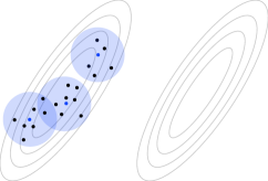
(a) Sample $S_{1}$ lie in a single mode. The minimum covering number for $\epsilon=1$ is $C_{\epsilon}(S_{1})=3$.

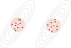
(b) Sample $S_{2}$ lie in two modes. The minimum covering number for $\epsilon=1$ is $C_{\epsilon}(S_{2})=2$.

Figure 2: Comparison of minimum covering numbers of samples ($\epsilon=1$)

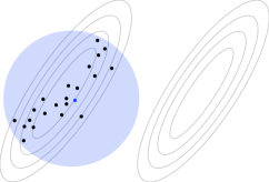
(a) Sample $S_{1}$ lie in a single mode. The minimum covering number for $\epsilon=2.5$ is $C_{\epsilon}(S_{1})=1$.

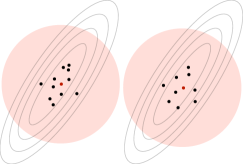
(b) Sample $S_{2}$ lie in two modes. The minimum covering number for $\epsilon=2.5$ is $C_{\epsilon}(S_{2})=2$.

Figure 3: Comparison of minimum covering numbers of samples ($\epsilon=2.5$)

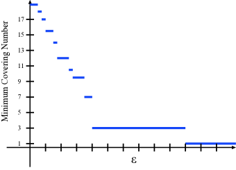
(a) The minimum covering number of $S_{1}$ persists at 3 for 6 $\Delta\epsilon$’s.

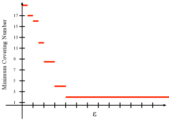
(b) The minimum covering number of $S_{1}$ persists at 2 for more than 9 $\Delta\epsilon$’s.

Figure 4: Comparison of persistent minimum covering numbers ($C_{\epsilon}$ as a function of $\epsilon$) of samples.

4 Case Study

In the following, we consider three different synthetic data sets with qualitatively different posterior structure: one with a single mode, one with two modes, and one with an infinite number of modes (or rather, a connected space of equally good solutions). We consider both a tiny version of the NMF problem, with only 4 or 5 observations and 6 or 7 dimensions, as well as larger one with 50 observations and 500 dimensions. We evaluate a number of sampling algorithms with various measures of “diversity”, running each algorithm for 10 repetitions of 10,000 samples. To avoid questions of whether samplers like Gibbs and HMC have mixed, we initialize them at one of the modes/maximum likelihood solutions.

4.1 Synthetic Data Sets

Unique Solution

Laurberg gives the following example, $X=WA$, where the NMF solution is a unique equivalence class of factorizations, for the value $a=0.3$.

$$W=\small\left(\begin{matrix}a&1&1&a&0&0\\ 1&a&0&0&a&1\\ 0&0&a&1&1&a\end{matrix}\right),\;\;A=W^{T}.\qquad$$ (6)

Under our Bayesian model, the posterior space of this NMF is unimodal.

Two Solutions

Simply by setting the value of $a$ to be $0.5$ in the previous example, Laurberg shows that $X$ will have two distinct solutions. In particular, these solutions are related by a change of basis matrix $Q$, so the two factorization cones are in the same subspace.

$$W=\small\left(\begin{matrix}0.5&1&1&0.5&0&0\\ 1&0.5&0&0&0.5&1\\ 0&0&0.5&1&1&0.5\end{matrix}\right),\;\;A=W^{T};\qquad Q=Q^{-1}=\frac{1}{3}\small\left(\begin{matrix}-1&2&2\\ 2&-1&2\\ 2&2&-1\end{matrix}\right).$$ (7)

Under our Bayesian model, the posterior space of this NMF is bimodal.

Infinite Solutions

Finally, for the following matrix,

$$X =\small\left(\begin{matrix}1&1&1&0&0&0&0&0&0\\ 0&0&0&1&1&1&0&0&0\\ 0&0&0&0&0&0&1&1&1\\ 1&0&0&1&0&0&1&0&0\\ 0&1&0&0&1&0&0&1&0\\ 0&0&1&0&0&1&0&0&1\\ 1&1&1&1&1&1&1&1&1\end{matrix}\right)$$ (8)

there are an infinite number of nonnegative factorizations. For any $\delta\in[0,1]$, we have $X=A_{\delta}W$, where

$$A_{\delta}=\small\left(\begin{matrix}1&0&0&0&0&0\\ 0&1&0&0&0&0\\ 0&0&1&0&0&0\\ 0&0&0&1&0&0\\ 0&0&0&0&1&0\\ 0&1&0&0&0&1\\ 1-\delta&1-\delta&1-\delta&\delta&\delta&\delta\end{matrix}\right),\quad W=\small\left(\begin{matrix}1&1&1&0&0&0&0&0&0\\ 0&0&0&1&1&1&0&0&0\\ 0&0&0&0&0&0&1&1&1\\ 1&0&0&1&0&0&1&0&0\\ 0&1&0&0&1&0&0&1&0\\ 0&0&1&0&0&1&0&0&1\\ \end{matrix}\right)$$ (9)

Under our Bayesian model, the posterior space of this NMF contains an infinite number of modes that form a connected subset of the parameter space.

4.1.1 Larger Data Sets

The above examples of data sets are valuable performing diagnostics on sampling algorithms and comparing diversity measures, because we know ground truth about the solution space for each example. The larger data sets we work with are simply high dimensional embeddings of these small data sets, chosen such that the desirable properties (such as the number of solutions) of the original data are preserved. To generate the larger data sets, we take a small $D\times N$ data $X$ and transform it using non-negative matrices $B_{1}$ and $B_{2}$ such that $X_{\text{large}}=B_{1}XB_{2}$. For an NMF data set, the factors transform in a simple manner: $A_{\text{large}}=B_{1}A$ and $W_{\text{large}}B_{2}$. In our experiments, the larger data sets have dimensions $D=500$ and $N=50$ (while relatively small, we show that even with data sets of this size samplers rarely move very far).

4.2 Inference Approaches

In constructing our chain of factorization matrices, we add Gaussian noise, with standard deviation $\sigma$, to the data matrix $X$, for which we know the exact factorizations. We call the noisy data $\widetilde{X}$.

Lower Bound: Single Mode

To provide a reasonable lower bound on coverage, we establish the single-mode baseline, wherein we generate a set of samples that only explore one mode or region. For this baseline, we fix one known exact solution, $X=WA$; to generate samples consistent with the Gaussian noise model, we initialize an NMF algorithm at $(W,A)$ and iteratively generate factorizations for the data $X$ with added Gaussian noise. The procedure is as follows: we initialize the multiplicative update algorithm of Lee and Seung Lee and Seung (1999) with $(W,A)$; we then run the algorithm for the data $\widetilde{X}+E_{i}$, where $E_{i}$ is the noise matrix for the additional Gaussian noise added at the $i^{\text{th}}$ iteration. In this fashion, we obtain variation in the entries of our factorization matrices (depending on the noise-level), but we know these variation is of a limited scale and that the chain contain samples from only one mode.

Upper Bound: All Modes

To provide a reasonable approximation of ideal coverage, we establish the all-modes baseline, wherein generates a set of samples that covers the entire solution space. At each iteration in the chain, we randomly pick one known exact solution. When the solutions are discrete, we uniformly sample them. In the infinite solutions case, we pick $\delta_{i}$ independently from the uniform distribution over [0,1]. We then apply the same perturb-and-factor methodology as in the single mode baseline to produce a set of factors that approximate the modes of the parameter space.

Gibbs

Schmidt et al propose a Bayesian approach to NMF in which each basis element $A_{d,r}$ and each weight $W_{r,n}$ is sampled independently from an exponential prior. Combined with a Gaussian likelihood, the updates for each element of $A$ and $W$ can be sampled element-wise from a rectified normal distribution, which is proportional to the product of a Gaussian and an exponential.

We initialize with a sample from the All Modes baseline so that no burn-in needed. We fix $\sigma$, the noise parameter in the Gaussian noise, as the same value used in generating $\widetilde{X}$.

Hamiltonian Monte Carlo

Hamiltonian Monte Carlo (HMC) is a Markov Chain Monte Carlo (MCMC) procedure that simulates Hamiltonian dynamics over the target distribution state space. The time-reversibility and volume preserving properties of the evolution of Hamiltonian systems ensure detailed balance Neal et al. (2011). By incorporating gradient information, HMC suppresses the random walk behavior which contributes to the inefficiency of many MCMC methods. Given a target density $\pi(q)$, we define a Hamiltonian of the form

$$H(q,p)=-\log\pi_{\mathcal{H}}(q)+\frac{1}{2}p^{\top}p$$ (10)

where $-\log\pi(q)$ is called the potential energy and the velocity, $p$, is given by a certain tangent vector at $q$. We simulate the dynamics with a discretized integrator, called the leap-frog integrator. Given an initial state $(q_{0},p_{0})$, a proposal state $(q_{n},p_{n})$ is reached by a series of steps in the direction of $\nabla_{q}\log\pi_{\mathcal{H}}(q)$ Byrne and Girolami (2013).

In the case of NMF, our target density, $\pi(W,A)$, is the log posterior distribution corresponding to our generative model. Since HMC have been demonstrated to be more successful than other MCMC methods in crossing multiple modes, for low-dimensional posterior spaces, one might expect HMC to out-perform Gibbs in finding multiple optima for NMF problems as well.

For our experiments, we implement HMC with adaptive step size and a fixed 100 leap count. We perform the HMC on the entry-wise log of the factor matrices in order to keep our solutions feasible. We initialize with a sample from the All Modes baseline and allow an additional burn-in period of 200 iterations so that the we can adaptively find a reasonable step-size.

Non-MCMC Baseline: (Filtered) Random Restarts

We run Lin’s projected gradient NMF algorithm Lin (2007) with random initializations. We expect this algorithm to explore multiple solutions when they exist because it is initialized at a random factor matrix each time. There are no asymptotic guarantees for exploring all solutions nor is there an underlying probabilistic framework. However, random restarts provides a baseline of how much coverage we might achieve in practice if we did not have access to the true solution but were not constrained to a probabilistic MCMC framework.

In practice, deterministic optimization algorithms such as the projected gradient algorithm are prone to get caught in very poor local optima Lin (2007). Thus, we report metrics for all random restart outputs as well as the subset of random restarts results that achieve likelihoods comparable with the other samplers (that is, we exclude random restarts results from local optima corresponding to very poor solutions). We call this second baseline filtered random restarts. In our experiments, we allow for reconstruction errors in the filtered samples to be up to ten times the maximum reconstruction error in the Gibbs chain.

4.3 Evalution Metrics

For our experiments, we report evaluation metrics measuring three key aspects of of sampling: quality of fit, sample independence and coverage of the parameter space.

Quality of Fit

We measure the quality of NMF solutions contained in a set of samples by computing the mean likelihood of the samples. Because methods like random restarts can produce samples from low-likelihood local optima that are widely distributed in the posterior space, the mean likelihood can be used to distinguish samples from multiple modes from those from multiple local optima.

Sample Independence

We measure the independence of the samples in a set using integrated autocorrelation time. Although sample independence can be assessed in a number of different ways, we choose to use only integrated autocorrelation time since previous work Cowles and Carlin (1996); Brooks and Roberts (1998a); Kass et al. (1998); Brooks and Roberts (1998b) have shown IAT to be a reasonable representative of this class of metrics.

Coverage

To asses the amount of coverage achieved by a set of samples, we compute the maximum pairwise distance, the mean pairwise distance, and the persistent minimum covering numbers. Furthermore, each metric of coverage is calculated with respect to both maximum angle similarity and $\ell_{1}$-minimum matching distance.

The persistent minimum covering numbers are computed over a range of 100 $\epsilon$ values and for the first 1000 elements of each chain. For each $\epsilon$ value, the minimum covering number we record is the mean of $C_{\epsilon}$ over 10 repetitions of the same experiment. As the set cover problem is NP-hard, we employ a greedy algorithm to approximate the coverage Chvatal (1979).

5 Results

Quality of Fit: Log-Likelihoods

By design, the one mode and all modes sampling algorithms fit the data well (see Table 1 in Appendix A and Table 5 in Appendix B). Since the Gibbs sampler the HMC sampler are initialized at a known mode, they also fit the data well while exploring the posterior space around that mode.

Random Restarts, on the other hand, has much lower likelihoods than the samplers. This result is expected (although perhaps not at this scale). It appears that, even on small toy data sets, Random Restarts is prone to being trapped in local optima around low-quality solutions. The presence of such poor factorizations in Random Restarts motivates the construction of the Filtered Random Restarts baseline, which contains the subset of Random Restart samples whose reconstruction error in the Frobenius norm $\|\widetilde{X}-AW\|_{F}$ falls within a fixed threshold. In constructing the filtered samples, we note that a large proportion of the Random Restarts samples from the toy-sized data sets fall within our allowable reconstruction criterion, while significantly fewer samples are allowed to filter through when we consider the larger $500\times 50$ data sets. In particular, the worst performance of Random Restarts is observed in the enlarged version of the bimodal data, wherein, within ten repetitions, the number of sample satisfying our filtering criteria ranged between 5 and 309 out of a total of 10,000 samples.

Sample Independence: IAT

The MCMC algorithms show high degrees of autocorrelation rendering the effective sample size of the 10,000 chain to be orders of magnitude smaller (Table 2 in Appendix A and Table 6 in Appendix B). Even on toy data sets with infinite number of connected solutions, the samples are highly correlated. As expected, the non-MCMC samples are effectively independent.

Coverage: Pairwise Distance and Minimum Covering Numbers

We note again that the likelihood and sample independence does not necessarily provide information about the region of the posterior that is being explored in these chains. For example, in the infinite solutions case, one can imagine a trajectory through the line of solutions parameterized by $\delta$ that could generate a set of samples with high autocorrelation but traverse along a large portion of the posterior. On the other hand, samples could appear uncorrelated when a chain is only making local but indpendent moves around a single mode. To assess coverage, we study the maximum/mean pairwise distance and persistent minimum covering numbers.

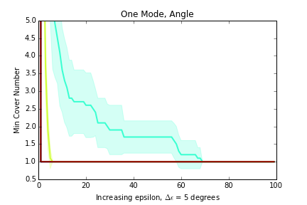
(a) Similarity measure: Max Angle

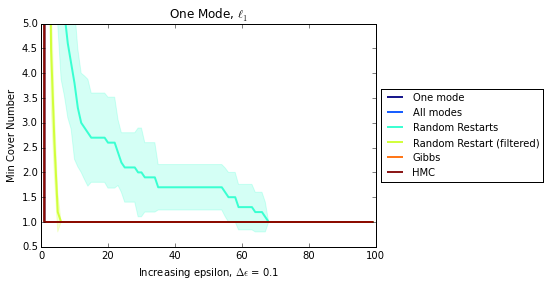
(b) Similarity measure: MinMatch ($\ell_{1}$)

Figure 5: Unique Mode

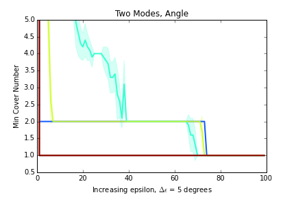
(a) Similarity measure: Max Angle

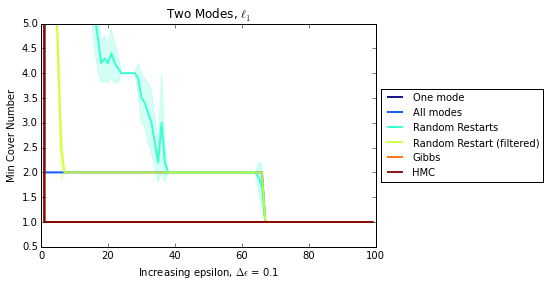
(b) Similarity measure: MinMatch ($\ell_{1}$)

Figure 6: Two Modes

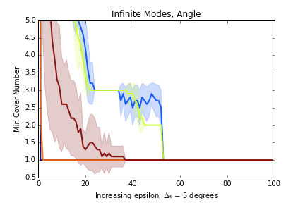
(a) Similarity measure: Max Angle

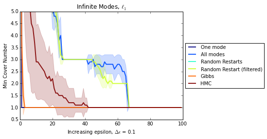
(b) Similarity measure: MinMatch ($\ell_{1}$)

Figure 7: Infinite modes

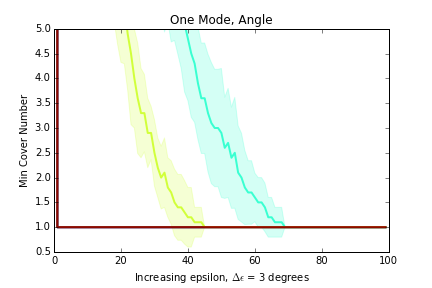
(a) Similarity measure: Max Angle

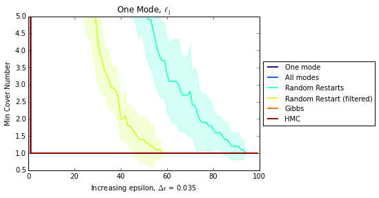
(b) Similarity measure: MinMatch ($\ell_{1}$)

Figure 8: Unique Mode

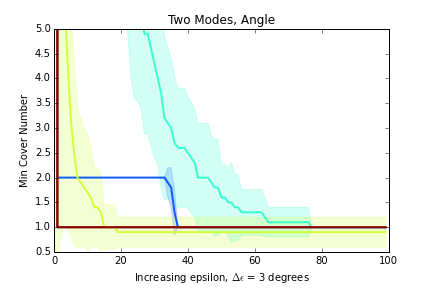
(a) Similarity measure: Max Angle

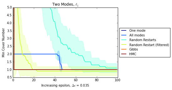
(b) Similarity measure: MinMatch ($\ell_{1}$)

Figure 9: Two Modes

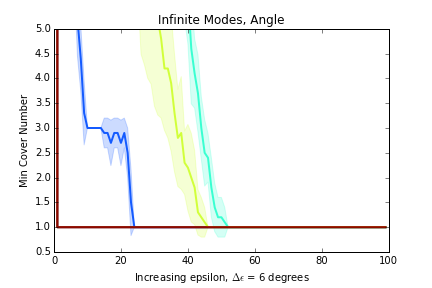
(a) Similarity measure: Max Angle

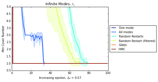
(b) Similarity measure: MinMatch ($\ell_{1}$)

Figure 10: Infinite modes

Both the pairwise distance measures (Table 3, Table 7, Table 4, Table 8) and the persistent covering numbers (Figures 5 - 10) indicate that Random Restarts obtains the widest range of solutions. However, because some (or many, depending on the data set) of the elements correspond to poor factorizations, they do not represent samples from multiple modes of the posterior space. Thus, the Filtered Random Restart samples reveals a better picture of the movement of this sampling algorithm through the posterior. The coverage metrics indicate that the Filtered Random Restart samples still explore significantly more of the posterior than the MCMC methods. In particular, in the toy sized bimodal data set, the Filtered Random Restart samples appears to sample from both modes.

The persistence covering number plots of the All Modes samples establish clear visual baselines for distinguishing sets containing samples from multiple modes in the posterior space. Comparing the plots of the Gibbs sampler and HMC against those of All Modes, we see these asymptotically correct sampling mechanisms tend to explore only a single mode (Figures 5 - 10).

6 Conclusion

We conclude from our experiments that the coverage metrics we introduce yield useful information regarding sampling behaviors that cannot be assessed using traditional MCMC diagnostics, such as the ability of the sampler to cover a large portion of the posterior space. We are able to evaluate and compare the exploratory behavior of chains through these metrics. Within the sampling algorithms we study, it appears that a filtered version of Random Restarts would show the best exploratory behavior while maintaining some quality of the factorization. In the data sets explored, the quality of the factorization deteriorates for Random Restarts as the scale of the data grows.

Both MCMC approaches, Gibbs and HMC, produce factorizations of excellent quality but IAT shows that effective sample size is very small. Furthermore, our coverage analysis reveals that neither Gibbs nor HMC are able to explore the multiple modes in very small toy data sets. As the scale of the data set grows, we expect the Gibbs sampler to be more vulnerable to becoming trapped in a single mode due of the local nature of its updates.

For the practitioner of NMF, these results first demonstrate that random restarts of some sort—such as running multiple chains—can still be important for covering the posterior space, even for very small problems. More importantly, we argue for adding coverage analysis of solutions to the standard diagnostic process evaluating sampling-based approches, since solution set diversity is an unavoidable questing arising from the identifiability of NMF and other problems. These multiple solutions can lead to very different interpretations of the data and effect subsequent modeling decisions. We hope that the metrics introduced in this work to quantify the notion of sample diversity begins to fill the gap left by current performance measurement of sampling algorithms.

Appendix A Comparison of Metrics and Algorithms (Small Dataset)

Table 1: Comparison of Performance of Sampling Method: Likelihood

		One Mode	All Modes	Random Restarts	Random Restarts (filtered)	Gibbs	HMC
One Mode		-1.74e+01	-1.74e+01	-1.12e+03	-2.30e+02	-2.38e+01	-1.93e+01
		-1.84e+01,	-1.84e+01,	-1.22e+03,	-2.34e+02,	-2.52e+01,	-2.02e+01,
		-1.73e+01,	-1.73e+01,	-1.09e+03,	-2.32e+02,	-2.46e+01,	-1.92e+01,
		-1.65e+01	-1.65e+01	-1.02e+03	-2.27e+02	-2.34e+01	-1.88e+01
Two Modes		-1.72e+01	-1.70e+01	-2.17e+03	-2.81e+02	-2.38e+01	-1.88e+01
		-1.80e+01,	-1.80e+01,	-2.24e+03,	-2.85e+02,	-2.51e+01,	-2.00e+01,
		-1.71e+01,	-1.69e+01,	-2.18e+03,	-2.79e+02,	-2.43e+01,	-1.93e+01,
		-1.62e+01	-1.63e+01	-2.07e+03	-2.77e+02	-2.32e+01	-1.75e+01
Infinite Modes		-2.20e+01	-2.18e+01	-1.20e+05	-3.20e+02	-4.21e+01	-2.09e+01
		-2.37e+01,	-2.31e+01,	-1.22e+05,	-3.23e+02,	-4.30e+01,	-2.20e+01,
		-2.18e+01,	-2.15e+01,	-1.21e+05,	-3.21e+02,	-4.17e+01,	-2.05e+01,
		-1.94e+01	-2.01e+01	-1.20e+05	-3.19e+02	-4.15e+01	-1.92e+01

Table 2: Comparison of Performance of Sampling Method: IAT

		One Mode	All Modes	Random Restarts	Random Restarts (filtered)	Gibbs	HMC
One Mode	IAT	1.009	1.009	1.014	1.014	728.498	837.699
		1.01,	1.01,	1.01,	1.01,	584.8875,	822.665,
		1.01,	1.01,	1.015,	1.015,	727.725,	865.465,
		1.01	1.01	1.02	1.02	850.7075	940.6925
Two Modes	IAT	1.009	1.004	1.013	1.013	677.867	813.753
		1.01,	1.0,	1.01,	1.01,	643.415,	726.395,
		1.01,	1.0,	1.01,	1.01,	686.235,	831.19,
		1.01	1.01	1.0175	1.0175	719.4575	890.53
Infinite Modes	IAT	1.008	1.008	1.009	1.009	313.22	710.851
		1.01,	1.01,	1.01,	1.01,	292.9875,	681.7575,
		1.01,	1.01,	1.01,	1.01,	306.475,	703.79,
		1.01	1.01	1.01	1.01	320.755	724.35

Table 3: Comparison of Performance of Sampling Method: Max

		One Mode	All Modes	Random Restarts	Random Restarts (filtered)	Gibbs	HMC
One Mode	Angle Max	0.185	0.185	34.763	4.184	0.289	0.221
		0.18,	0.18,	28.395,	3.995,	0.28,	0.21,
		0.18,	0.18,	39.565,	4.055,	0.285,	0.215,
		0.19	0.19	39.6225	4.315	0.2975	0.2275
	MM $\ell_{1}$ Max	0.0	0.0	0.697	0.091	0.01	0.0
		0.0,	0.0,	0.575,	0.09,	0.01,	0.0,
		0.0,	0.0,	0.79,	0.09,	0.01,	0.0,
		0.0	0.0	0.79	0.09	0.01	0.0
Two Modes	Angle Max	0.152	36.965	38.132	37.895	0.278	0.219
		0.15,	36.9525,	37.8775,	37.7375,	0.27,	0.21,
		0.15,	36.96,	37.915,	37.89,	0.28,	0.21,
		0.15	36.9775	38.155	37.95	0.2875	0.2275
	MM $\ell_{1}$ Max	0.0	0.67	0.738	0.694	0.01	0.0
		0.0,	0.67,	0.73,	0.69,	0.01,	0.0,
		0.0,	0.67,	0.73,	0.69,	0.01,	0.0,
		0.0	0.67	0.7375	0.7	0.01	0.0
Infinite Modes	Angle Max	0.187	44.973	90.0	44.99	1.187	16.229
		0.18,	44.9375,	90.0,	44.9725,	0.985,	6.625,
		0.185,	44.975,	90.0,	44.99,	1.115,	17.605,
		0.1975	45.0075	90.0	44.9975	1.355	22.2925
	MM $\ell_{1}$ Max	0.009	1.0	2.0	1.004	0.032	0.383
		0.01,	1.0,	2.0,	1.0,	0.0225,	0.1825,
		0.01,	1.0,	2.0,	1.0,	0.03,	0.425,
		0.01	1.0	2.0	1.01	0.04	0.52

Table 4: Comparison of Performance of Sampling Method: Mean

		One Mode	All Modes	Random Restarts	Random Restarts (filtered)	Gibbs	HMC
One Mode	Angle Mean	0.069	0.069	0.873	0.615	0.11	0.09
		0.07,	0.07,	0.75,	0.6,	0.11,	0.09,
		0.07,	0.07,	0.89,	0.61,	0.11,	0.09,
		0.07	0.07	0.985	0.6275	0.11	0.09
	MM $\ell_{1}$ Mean	0.0	0.0	0.019	0.01	0.0	0.0
		0.0,	0.0,	0.02,	0.01,	0.0,	0.0,
		0.0,	0.0,	0.02,	0.01,	0.0,	0.0,
		0.0	0.0	0.02	0.01	0.0	0.0
Two Modes	Angle Mean	0.06	18.467	18.61	18.563	0.102	0.089
		0.06,	18.4725,	18.6025,	18.5625,	0.1,	0.09,
		0.06,	18.48,	18.615,	18.575,	0.1,	0.09,
		0.06	18.4875	18.6275	18.58	0.1	0.09
	MM $\ell_{1}$ Mean	0.0	0.33	0.34	0.34	0.0	0.0
		0.0,	0.33,	0.34,	0.34,	0.0,	0.0,
		0.0,	0.33,	0.34,	0.34,	0.0,	0.0,
		0.0	0.33	0.34	0.34	0.0	0.0
Infinite Modes	Angle Mean	0.078	16.572	27.261	12.835	0.371	5.16
		0.08,	16.485,	26.6225,	12.3425,	0.2925,	1.65,
		0.08,	16.525,	27.33,	12.725,	0.315,	5.62,
		0.08	16.6775	27.69	13.3525	0.4425	6.1625
	MM $\ell_{1}$ Mean	0.0	0.373	0.566	0.284	0.011	0.123
		0.0,	0.37,	0.56,	0.27,	0.01,	0.0425,
		0.0,	0.37,	0.56,	0.28,	0.01,	0.135,
		0.0	0.3775	0.57	0.2975	0.01	0.1475

Appendix B Comparison of Metrics and Algorithms (Large Dataset)

Table 5: Comparison of Performance of Sampling Method: Likelihood

		One Mode	All Modes	Random Restarts	Random Restarts (filtered)	Gibbs	HMC
One Mode		-1.22e+04	-1.22e+04	-1.68e+06	-1.00e+06	-1.25e+04	-1.25e+04
		-1.23e+04,	-1.23e+04,	-1.82e+06,	-1.04e+06,	-1.26e+04,	-1.26e+04,
		-1.22e+04,	-1.22e+04,	-1.63e+06,	-9.99e+05,	-1.24e+04,	-1.24e+04,
		-1.22e+04	-1.22e+04	-1.50e+06	-9.57e+05	-1.24e+04	-1.24e+04
Two Modes		-1.22e+04	-1.22e+04	-3.60e+06	-1.09e+06	-1.25e+04	-1.25e+04
		-1.23e+04,	-1.23e+04,	-3.74e+06,	-1.14e+06,	-1.26e+04,	-1.26e+04,
		-1.22e+04,	-1.22e+04,	-3.55e+06,	-1.10e+06,	-1.24e+04,	-1.24e+04,
		-1.22e+04	-1.22e+04	-3.21e+06	-1.04e+06	-1.24e+04	-1.24e+04
Infinite Modes		-1.20e+04	-1.20e+04	-1.82e+06	-9.98e+05	-1.25e+04	-1.25e+04
		-1.20e+04,	-1.20e+04,	-1.94e+06,	-1.01e+06,	-1.25e+04,	-1.25e+04,
		-1.20e+04,	-1.20e+04,	-1.82e+06,	-9.93e+05,	-1.25e+04,	-1.25e+04,
		-1.20e+04	-1.19e+04	-1.65e+06	-9.73e+05	-1.24e+04	-1.24e+04

Table 6: Comparison of Performance of Sampling Method: IAT

		One Mode	All Modes	Random Restarts	Random Restarts (filtered)	Gibbs	HMC
One Mode	IAT	1.01	1.01	1.011	1.009	645.903	1173.558
		1.01,	1.01,	1.0025,	1.0025,	600.07,	1115.425,
		1.01,	1.01,	1.01,	1.01,	649.92,	1186.735,
		1.01	1.01	1.0175	1.01	694.5775	1286.695
Two Modes	IAT	1.01	1.011	1.012	1.082	524.915	1105.867
		1.01,	1.01,	1.0025,	1.0625,	434.6325,	1046.2725,
		1.01,	1.02,	1.01,	1.1,	530.575,	1124.91,
		1.01	1.02	1.02	1.1175	563.32	1180.215
Infinite Modes	IAT	1.01	1.008	1.005	1.014	1067.452	1077.456
		1.01,	1.0,	1.0,	1.0025,	1059.7475,	1071.205,
		1.01,	1.0,	1.005,	1.01,	1068.9,	1076.965,
		1.01	1.025	1.01	1.02	1077.79	1086.3875

Table 7: Comparison of Performance of Sampling Method: Max

		One Mode	All Modes	Random Restarts	Random Restarts (filtered)	Gibbs	HMC
One Mode	Angle Max	0.01	0.01	25.504	16.326	0.027	0.092
		0.01,	0.01,	22.93,	14.705,	0.0225,	0.08,
		0.01,	0.01,	25.68,	16.315,	0.03,	0.09,
		0.01	0.01	28.15	17.7075	0.03	0.0975
	MM $\ell_{1}$ Max	0.0	0.0	0.444	0.258	0.0	0.0
		0.0,	0.0,	0.4025,	0.24,	0.0,	0.0,
		0.0,	0.0,	0.44,	0.255,	0.0,	0.0,
		0.0	0.0	0.4825	0.285	0.0	0.0
Two Modes	Angle Max	0.01	10.779	22.131	5.084	0.02	0.072
		0.01,	10.6525,	17.6125,	3.405,	0.02,	0.07,
		0.01,	10.69,	23.08,	4.51,	0.02,	0.07,
		0.01	11.0125	26.05	6.765	0.02	0.0775
	MM $\ell_{1}$ Max	0.0	0.16	0.382	0.075	0.0	0.0
		0.0,	0.16,	0.2825,	0.05,	0.0,	0.0,
		0.0,	0.16,	0.4,	0.07,	0.0,	0.0,
		0.0	0.16	0.44	0.1	0.0	0.0
Infinite Modes	Angle Max	0.01	21.412	42.943	35.901	0.202	0.556
		0.01,	21.2,	41.9175,	33.4125,	0.19,	0.525,
		0.01,	21.41,	42.99,	35.68,	0.2,	0.555,
		0.01	21.6175	43.86	38.1225	0.225	0.5875
	MM $\ell_{1}$ Max	0.0	0.348	0.985	0.796	0.0	0.01
		0.0,	0.3425,	0.93,	0.7325,	0.0,	0.01,
		0.0,	0.35,	0.98,	0.785,	0.0,	0.01,
		0.0	0.35	1.0375	0.8375	0.0	0.01

Table 8: Comparison of Performance of Sampling Method: Mean

		One Mode	All Modes	Random Restarts	Random Restarts (filtered)	Gibbs	HMC
One Mode	Angle Mean	0.01	0.01	5.172	4.293	0.02	0.041
		0.01,	0.01,	4.7825,	4.15,	0.02,	0.04,
		0.01,	0.01,	5.075,	4.235,	0.02,	0.04,
		0.01	0.01	5.635	4.29	0.02	0.04
	MM $\ell_{1}$ Mean	0.0	0.0	0.077	0.062	0.0	0.0
		0.0,	0.0,	0.07,	0.06,	0.0,	0.0,
		0.0,	0.0,	0.075,	0.06,	0.0,	0.0,
		0.0	0.0	0.08	0.06	0.0	0.0
Two Modes	Angle Mean	0.01	5.38	3.467	2.457	0.02	0.033
		0.01,	5.33,	3.1325,	1.97,	0.02,	0.03,
		0.01,	5.35,	3.44,	2.75,	0.02,	0.03,
		0.01	5.49	3.8375	3.0	0.02	0.04
	MM $\ell_{1}$ Mean	0.0	0.08	0.051	0.036	0.0	0.0
		0.0,	0.08,	0.05,	0.03,	0.0,	0.0,
		0.0,	0.08,	0.05,	0.04,	0.0,	0.0,
		0.0	0.08	0.0575	0.04	0.0	0.0
Infinite Modes	Angle Mean	0.01	7.935	16.088	11.978	0.108	0.307
		0.01,	7.8125,	15.7175,	11.665,	0.1,	0.285,
		0.01,	7.905,	15.87,	11.885,	0.105,	0.305,
		0.01	8.0175	16.6375	12.16	0.1175	0.32
	MM $\ell_{1}$ Mean	0.0	0.129	0.258	0.186	0.0	0.001
		0.0,	0.13,	0.25,	0.18,	0.0,	0.0,
		0.0,	0.13,	0.26,	0.185,	0.0,	0.0,
		0.0	0.13	0.2675	0.19	0.0	0.0

Appendix C Persistent Minimum Covering Number Plots (Small Dataset)

Appendix D Persistent Minimum Covering Number Plots (Large Dataset)

References

- Liu (1996) J. S. Liu, “Metropolized independent sampling with comparisons to rejection sampling and importance sampling,” Statistics and Computing, vol. 6, no. 2, pp. 113–119, 1996.
- Halton (1962) J. H. Halton, “Sequential monte carlo,” in Mathematical Proceedings of the Cambridge Philosophical Society, vol. 58, no. 01. Cambridge Univ Press, 1962, pp. 57–78.
- Gilks (2005) W. R. Gilks, Markov chain monte carlo. Wiley Online Library, 2005.
- Wainwright and Jordan (2008) M. J. Wainwright and M. I. Jordan, “Graphical models, exponential families, and variational inference,” Foundations and Trends® in Machine Learning, vol. 1, no. 1-2, pp. 1–305, 2008.
- Tzikas et al. (2008) D. G. Tzikas, A. C. Likas, and N. P. Galatsanos, “The variational approximation for bayesian inference,” IEEE Signal Processing Magazine, vol. 25, no. 6, pp. 131–146, 2008.
- Opper and Archambeau (2009) M. Opper and C. Archambeau, “The variational gaussian approximation revisited,” Neural computation, vol. 21, no. 3, pp. 786–792, 2009.
- Johnson (1996) V. E. Johnson, “Studying convergence of markov chain monte carlo algorithms using coupled sample paths,” Journal of the American Statistical Association, vol. 91, no. 433, pp. 154–166, 1996.
- Cowles and Carlin (1996) M. K. Cowles and B. P. Carlin, “Markov chain monte carlo convergence diagnostics: a comparative review,” Journal of the American Statistical Association, vol. 91, no. 434, pp. 883–904, 1996.
- Flegal et al. (2010) J. M. Flegal, G. L. Jones et al., “Batch means and spectral variance estimators in markov chain monte carlo,” The Annals of Statistics, vol. 38, no. 2, pp. 1034–1070, 2010.
- Brooks (1998) S. P. Brooks, “Quantitative convergence assessment for markov chain monte carlo via cusums,” Statistics and Computing, vol. 8, no. 3, pp. 267–274, 1998.
- (11) D. Aldous and J. Fill, “Reversible markov chains and random walks on graphs.”
- Lee et al. (2015) C.-H. Lee et al., “On the efficiency-optimal markov chains for distributed networking applications,” in 2015 IEEE Conference on Computer Communications (INFOCOM). IEEE, 2015, pp. 1840–1848.
- Greene et al. (2008) D. Greene, G. Cagney, N. Krogan, and P. Cunningham, “Ensemble non-negative matrix factorization methods for clustering protein–protein interactions,” Bioinformatics, 2008.
- Roberts et al. (2016) M. E. Roberts, B. M. Stewart, and D. Tingley, “Navigating the local modes of big data,” Computational Social Science, p. 51, 2016.
- Brunet et al. (2004) J.-P. Brunet, P. Tamayo, T. R. Golub, and J. P. Mesirov, “Metagenes and molecular pattern discovery using matrix factorization,” PNAS, vol. 101, no. 12, pp. 4164–4169, 2004.
- Paisley et al. (2015) J. Paisley, D. M. Blei, and M. I. Jordan, “Bayesian nonnegative matrix factorization with stochastic variational inference,” Handbook of Mixed Membership Models and Their Applications. Chapman and Hall/CRC, 2015.
- Schmidt et al. (2009) M. N. Schmidt, O. Winther, and L. K. Hansen, “Bayesian non-negative matrix factorization,” in Independent Component Analysis and Signal Separation. Springer, 2009, pp. 540–547.
- Moussaoui et al. (2006) S. Moussaoui, D. Brie, A. Mohammad-Djafari, and C. Carteret, “Separation of non-negative mixture of non-negative sources using a bayesian approach and mcmc sampling,” Signal Processing, IEEE Transactions on, vol. 54, no. 11, pp. 4133–4145, 2006.
- Lin (2007) C.-J. Lin, “Projected gradient methods for nonnegative matrix factorization,” Neural computation, vol. 19, no. 10, pp. 2756–2779, 2007.
- Lee and Seung (2001) D. D. Lee and H. S. Seung, “Algorithms for non-negative matrix factorization,” in Advances in neural information processing systems, 2001, pp. 556–562.
- Recht et al. (2012) B. Recht, C. Re, J. Tropp, and V. Bittorf, “Factoring nonnegative matrices with linear programs,” in Advances in Neural Information Processing Systems, 2012, pp. 1214–1222.
- Walters (2011) M. Walters, “Random geometric graphs,” in Surveys in Combinatorics 2011, London Mathematical Society Lecture Note Series, vol. 392, 2011.
- Kriegel et al. (2003) H.-P. Kriegel, S. Brecheisen, P. Kröger, M. Pfeifle, and M. Schubert, “Using sets of feature vectors for similarity search on voxelized cad objects,” in Proceedings of the 2003 ACM SIGMOD international conference on Management of data. ACM, 2003, pp. 587–598.
- (24) S. Brecheisen, H.-P. Kriegel, and M. Pfeifle, “Efficient similarity search on vector sets,” preprint.
- Masood and Doshi-Velez (2016) M. Masood and F. Doshi-Velez, “Faster mixing of bayesian non-negative matrix factorization using geometrically inspired metropolis hastings proposals within gibbs sampler,” Feburary 2016, preprint.
- Abbott and Liu (1979) H. Abbott and A. Liu, “Bounds for the covering number of a graph,” Discrete Mathematics, vol. 25, no. 3, pp. 281–284, 1979.
- Chepoi et al. (2007) V. Chepoi, B. Estellon, and Y. Vaxes, “Covering planar graphs with a fixed number of balls,” Discrete & Computational Geometry, vol. 37, no. 2, pp. 237–244, 2007.
- Edelsbrunner and Harer (2008) H. Edelsbrunner and J. Harer, “Persistent homology-a survey,” Contemporary mathematics, vol. 453, pp. 257–282, 2008.
- Carlsson (2009) G. Carlsson, “Topology and data,” Bulletin of the American Mathematical Society, vol. 46, no. 2, pp. 255–308, 2009.
- Ghrist (2008) R. Ghrist, “Barcodes: the persistent topology of data,” Bulletin of the American Mathematical Society, vol. 45, no. 1, pp. 61–75, 2008.
- Lee and Seung (1999) D. Lee and H. Seung, “Learning the parts of objects by nonnegative matrix factorization,” Nature, vol. 401, pp. 788–791, 1999.
- Neal et al. (2011) R. M. Neal et al., “Mcmc using hamiltonian dynamics,” Handbook of Markov Chain Monte Carlo, vol. 2, pp. 113–162, 2011.
- Byrne and Girolami (2013) S. Byrne and M. Girolami, “Geodesic monte carlo on embedded manifolds,” Scandinavian Journal of Statistics, vol. 40, no. 4, pp. 825–845, 2013.
- Brooks and Roberts (1998a) S. P. Brooks and G. O. Roberts, “Assessing convergence of markov chain monte carlo algorithms,” Statistics and Computing, vol. 8, no. 4, pp. 319–335, 1998.
- Kass et al. (1998) R. E. Kass, B. P. Carlin, A. Gelman, and R. M. Neal, “Markov chain monte carlo in practice: a roundtable discussion,” The American Statistician, vol. 52, no. 2, pp. 93–100, 1998.
- Brooks and Roberts (1998b) S. P. Brooks and G. O. Roberts, “Convergence assessment techniques for markov chain monte carlo,” Statistics and Computing, vol. 8, no. 4, pp. 319–335, 1998.
- Chvatal (1979) V. Chvatal, “A greedy heuristic for the set-covering problem,” Mathematics of operations research, vol. 4, no. 3, pp. 233–235, 1979.