Published in Phys. Rev. B 96, 064511 (2016) [doi:10.1103/PhysRevB.94.064511]
Electron bubbles and Weyl Fermions in chiral superfluid ³He-A

Abstract

Electrons embedded in liquid ³He form mesoscopic bubbles with radii large compared to the interatomic distance between ³He atoms, voids of $N_{\text{bubble}}\approx 200$ ³He atoms, generating a negative ion with a large effective mass that scatters thermal excitations. Electron bubbles in chiral superfluid ³He-A also provide a local probe of the ground state. We develop scattering theory of Bogoliubov quasiparticles by negative ions embedded in ³He-A that incorporates the broken symmetries of ³He-A, particularly broken symmetries under time-reversal and mirror symmetry in a plane containing the chiral axis $\hat{\mathbf{l}}$. Multiple scattering by the ion potential, combined with branch conversion scattering by the chiral order parameter, leads to a spectrum of Weyl Fermions bound to the ion that support a mass current circulating the electron bubble - the mesoscopic realization of chiral edge currents in superfluid ³He-A films. A consequence is that electron bubbles embedded in ³He-A acquire angular momentum, $\mathbf{L}\approx-(N_{\text{bubble}}/2)\hbar\,\hat{\mathbf{l}}$, inherited from the chiral ground state. We extend the scattering theory to calculate the forces on a moving electron bubble, both the Stokes drag and a transverse force, $\mathbf{F}_{\text{W}}=\frac{e}{c}\mathbf{v}\times\mathbf{B}_{\text{W}}$, defined by an effective magnetic field, $\mathbf{B}_{\text{W}}\propto\hat{\mathbf{l}}$, generated by the scattering of thermal quasiparticles off the spectrum of Weyl Fermions bound to the moving ion. The transverse force is responsible for the anomalous Hall effect for electron bubbles driven by an electric field reported by the RIKEN group. Our results for the scattering cross section, drag and transverse forces on moving ions are compared with experiments, and shown to provide a quantitative understanding of the temperature dependence of the mobility and anomalous Hall angle for electron bubbles in normal and superfluid ³He-A. We also discuss our results in relation to earlier work on the theory of negative ions in superfluid ³He.

I Introduction

A unique feature of the chiral phase of superfluid ³He, predicted early on by Anderson and Morel (AM), is that this fluid should possess a macroscopic ground-state angular momentum, $\mathbf{L}=L_{z}\,\hat{\mathbf{l}}$,Anderson and Morel (1960); Volovik (1975); Cross (1977); Ishikawa (1977); Leggett and Takagi (1978); McClure and Takagi (1979) where $\hat{\mathbf{l}}$ is the chiral axis along which the Cooper pairs have angular momentum $\hbar$. Ground state currents and angular momentum are signatures of broken time-reversal and parity (BTRP) derived from the orbital motion of the Cooper pairs in ³He-A. In this article we discuss signatures of BTRP generated by the structure of electrons embedded in superfluid ³He-A. An electron forms a void, a “bubble”, in liquid ³He-A that disturbs the chiral ground state.Rainer and Vuorio (1977) We show that multiple scattering of Bogoliubov quasiparticles off the electron bubble leads to the formation of chiral Fermions bound to the electron bubble, and to a ground state angular momentum and mass current circulating each electron bubble. Indeed the electron bubble provides a mesocopic realization of chiral edge currents in superfluid ³He-A. A main result of the work reported here is our formulation of transport theory for negative ions that correctly accounts for the chiral symmetry of superfluid ³He-A. This allows us to show that the chiral structure of the electron bubble in ³He-A provides a quantitative theory for the anomalous Hall effect reported by Ikegami et al. Ikegami et al. (2013, 2015) We start with a brief introduction intended to make the connection between ground state currents, angular momentum, and chiral edge states in ³He-A, with the structure of electron bubbles in ³He-A.

The angular momentum of bulk ³He-A has so far not been measured, perhaps in part because of variations in the literature on the magnitute of $L_{z}$ (c.f. Ref. [Sauls, 2011] and references therein). McClure and Takagi (MT) obtained the result, $L_{z}=(N/2)\,\hbar$, for $N$ atoms confined in a container of volume $V$ with cylindrical symmetry, and condensed into a chiral p-wave bound state of Fermion pairs. This result is independent of whether or not the ground state is a condensate of overlapping chiral Cooper pairs ($\xi\gg a$) or a Bose-Einstein condensate of tightly bound chiral molecules ($\xi\ll a$), where $\xi$ represents the radial extent of the pair wave function, $a=1/\sqrt[3]{n}$ is the interatomic spacing and $n$ is the mean atomic density. While the MT result is in accord with expectations for a BEC of $N/2$ chiral molecules, the MT result for the BCS limit suggests that the currents responsible for a ground-state angular momentum of $(N/2)\hbar$ are confined on the boundary walls.Volovik and Mineev (1981); Sauls (2011)

The existence of currents confined on the boundary is a natural conclusion of the bulk-boundary correspondence for a topological phase with broken time-reversal symmetry.Hatsugai (1993); Volovik (2016); Mizushima et al. (2016) In the quasi-2D limit the chiral A-phase is fully gapped and belongs to a topological class related to that of integer quantum Hall systems.Read and Green (2000); Volovik (1988, 1992a) The topology of the chiral AM state requires gapless Weyl fermions confined on the edge of a thin film of superfluid ³He-A.Volovik (1992a, b) For an isolated boundary a branch of Weyl fermions disperses linearly with momentum $p_{||}$ along the boundary, i.e. $\varepsilon(p_{||})=c\,p_{||}$, where $c=v_{f}\,|\Delta|/E_{f}\ll v_{f}$ is the velocity of the Weyl Fermions. The asymmetry of the Weyl branch under time-reversal, $\varepsilon(-p_{||})=-\varepsilon(p_{||})$, implies the existence of a ground-state edge current derived from the occupation of the negative energy states.Stone and Roy (2004); Sauls (2011) For ³He-A confined in a thin cylindrical cavity, or a film, the chiral edge current on the outer boundary edge, $J=\genfrac{}{}{}{1}{1}{4}\,n\,\hbar$, is the source of the ground-state angular momentum, $L_{z}=(N/2)\,\hbar$, predicted by MT.Sauls (2011); Tsutsumi and Machida (2012); Stone and Roy (2004)

To reveal the edge currents, consider an unbounded thin film of superfluid ³He-A with a circular barrier, a “hole”, excluding ³He as shown in Fig. (1). The edge current is confined to the boundary on the scale of $\xi_{\mbox{\small$\Delta$}}=\hbar v_{f}/2\Delta\approx 100\,\mbox{nm}$. The angular momentum resulting from the edge current circulating the hole is, $L_{z}=-(N_{\text{hole}}/2)\,\hbar$, which is opposite to the chirality of the ground state Cooper pairs, and with magnitude given by $N_{\text{hole}}=n\,\pi\,R^{2}\,w$, the number of ³He atoms excluded by the hole of radius $R$ and thickness $w$. Nature provides us with such a “hole” in the form of an electron bubble to reveal the BTRP of ³He-A, and to probe the spectrum of chiral edge states, the mass current circulating the electron bubble, and the effect of the chiral edge states on the tranport properties of the electron bubble in ³He-A.

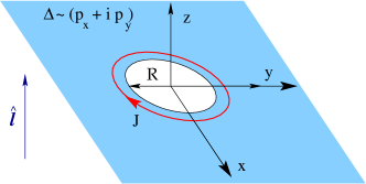
Figure 1: (Color online) An unbounded ³He-A film with an inner boundary of radius $R\gg\xi_{0}$. A ground-state edge current of magnitude $J=\genfrac{}{}{}{1}{1}{4}\,n\,\hbar$ circulates on the inner boundary generating an angular momentum $L_{z}=-(N_{\text{hole}}/2)\,\hbar$ with $N_{\text{hole}}=n\,\pi\,R^{2}\,w$, i.e. the number of ³He atoms excluded by the hole.

We begin with the structure of the electron bubble in the normal Fermi liquid phase of ³He in Sec. (II). The normal-state $t$-matrix and scattering phase shifts for quasiparticles scattering off the electron bubble are central to understanding the properties of the electron bubble in superfluid ³He-A. In Sec. (III) we develop scattering theory to calculate the spectrum of chiral Fermions bound to the electron bubble in ³He-A. We present results for the mass current and orbital angular momentum obtained from the Fermionic spectrum. The momentum and energy resolved differential cross section for the scattering of Bogoliubov quasiparticles is developed in Sec. (IV), and used to calculate the forces on electron bubbles moving in the chiral phase of superfluid ³He. We present new theoretical predictions and analysis for the drag force on electron bubbles in ³He-A, and particularly the transverse force responsible for the anomalous Hall current of electron bubbles in superfluid ³He-A. In Sec. (V) we present the quantitative comparison of our theory with the measurements of the drag force and anomalous Hall effect reported by Ikegami et al. Ikegami et al. (2013, 2015) Our analysis establishes that the observation of the anomalous Hall effect for negative ions is not only a signature of BTRP, but a signature of chiral Fermions circulating the electron bubble.

We point out that previous theories for the mobility of ions in superfluid ³He-A start from an implicit assumption of mirror symmetry in the formulation of the transport cross-section for scattering of quasiparticles off the electron bubble. Specifically, in Sec. (IV.2) and App. (A) we discuss our theory in relation to the earlier theoretical works of Salomaa et al.Salomaa et al. (1980) and Salmelin et al.,Salmelin et al. (1989); Salmelin and Salomaa (1990) and point out that these earlier theoretical works give zero Hall mobility (Ref. [Salmelin and Salomaa, 1990]), or report a spurious Hall mobility that is an artefact of an error in evaluating the kinematics for the scattering of quasiparticles off the ion. As a result, the theory reported in Refs. [Salmelin et al., 1989; Salmelin and Salomaa, 1990] not only predicts a spurious Hall mobility in ³He-A, but also a spurious anisotropic mobility in normal liquid ³He.

Our formulation of the transport theory correctly accounts for the chiral symmetry of superfluid ³He-A, which is at the root of the anomalous Hall effect for electrons in ³He-A, and as shown in Sec. (V.3) is in quantitative agreement with the experimental measurements reported in Refs. [Ikegami et al., 2013, 2015].

II Electron bubbles in Liquid ³He

Electrons experience a repulsive barrier $\approx 1\,\mbox{eV}$ at the surface of liquid Helium.Woolf and Rayfield (1965) When an electric field pushes the electron into Helium the combination of the barrier, the surface tension and zero-point kinetic energy of the electron conspire to form a self-trapped electron in a spherical void of radius $R$, an “electron bubble”.Ferrell (1957); Kuper (1961); Fetter (1976); Dobbs (2000) The basic model of an electron bubble in liquid ³He is based on an energy function that consists of three terms,Ferrell (1957); Ahonen et al. (1978)

$$E(R,P)=E_{0}(U_{0},R)+4\pi R^{2}\gamma+\frac{4\pi}{3}R^{3}P,$$ (1)

where $\gamma=0.15\,\mathrm{erg/cm^{2}}$ is the surface tension of ³He,LoveJoy (1955); Suzuki et al. (1988) $P$ is the external pressure and $E_{0}$ is the ground state energy of the electron bubble trapped in an isotropic potential of radius $R$ and depth $-U_{0}$. In the limit $U_{0}\rightarrow\infty$, $E_{0}=-U_{0}+\pi^{2}\hbar^{2}/2m_{e}\,R^{2}$ is the energy of the electron of mass $m_{e}$ in its ground state. The balance between the surface tension of liquid ³He, the external pressure and the kinetic energy of the confined electron determines the bubble radius, $P={\pi\hbar^{2}}/{4m_{e}R^{5}}-{2\gamma}/{R}$. For zero pressure the radius is then

$$R=\left(\frac{\pi\hbar^{2}}{8m_{e}\gamma}\right)^{\genfrac{}{}{}{1}{1}{4}}\approx 2.38\,\mbox{nm}\,.$$ (2)

The bubble radius is large compared to the Fermi wavelength of ³He quasiparticles, $\lambda_{f}=1/k_{f}=0.127\,\mbox{nm}$, set by the ³He density, but is small compared to the Cooper pair correlation length, $\xi_{0}=\hbar v_{f}/2\pi\,k_{B}T_{c}\approx 77.3\,\mbox{nm}$. It is useful to refer to the dimensionless ratio, $k_{f}R$, which for the infinte barrier limit is $k_{f}R=18.67$ at $P=0$. Models for the confining potential with a finite pressure-dependent $U_{0}\sim 1\,\mbox{eV}$ yield a slightly smaller radius of $k_{f}R\approx 16.74$.Ahonen et al. (1978)

II.1 Electron Mobility in Normal ³He

A different measure of the size of the electron bubble may be obtained from the scattering of ³He quasiparticles off the electron bubble, i.e. the total cross section presented to quasiparticles with momenta and energies near the Fermi surface. The scattering of quasiparticles off the heavy electron bubble determines the mobility of the electron bubble. The heavy mass of the ion and large cross section for quasiparticle collisions imply that the scattering of quasiparticles off the electron bubble is nearly elastic.Josephson and Lekner (1969); Fetter and Kurkijärvi (1977) The mobility of the electron bubble in normal ³He is then temperature independent over the range $T_{c}<T<T_{0}=\hbar^{2}k_{f}^{2}/2M\approx 30\,\mbox{mK}$, and given by

$$\frac{e}{\mu_{\text{N}}}=n_{3}p_{f}\sigma_{\text{N}}^{\text{tr}}\,,\quad\sigma_{\text{N}}^{\text{tr}}=\int d\Omega_{\hat{\mathbf{k}}^{\prime}}\frac{d\sigma}{d\Omega_{\hat{\mathbf{k}}^{\prime}}}\left(1-\hat{\mathbf{k}}^{\prime}\cdot\hat{\mathbf{k}}\right)\,,$$ (3)

where $\sigma_{\text{N}}^{\text{tr}}$ is the transport cross section for elastic scattering of quasiparticles off an electron bubble, and

$$\frac{d\sigma}{d\Omega_{\hat{\mathbf{k}}^{\prime}}}=\left|\frac{m^{*}}{2\pi\hbar^{2}}\,t^{\text{R}}_{\text{N}}(\hat{\mathbf{k}}^{\prime},\hat{\mathbf{k}};E)\right|^{2}\,,$$ (4)

is the differential cross-section defined by the on-shell $t$-matrix for normal-state quasiparticles with effective mass $m^{*}$ scattering off a static electron bubble.

The full $t$-matrix obeys the Lippmann-Schwinger equation, $T_{\text{N}}^{\text{R}}=V+VG_{\text{N}}^{\text{R}}T_{\text{N}}^{\text{R}}$, where $G^{\text{R}}_{\text{N}}$ is the retarded propagator for Fermions in the normal Fermi liquid. At temperatures $k_{\text{B}}T\ll E_{f}$ the properties of ³He are dominated by quasiparticles with momenta near the Fermi surface, $\mathbf{k}\simeq k_{f}\hat{\mathbf{k}}$, and excitation energies, $\xi_{\mathbf{k}}\simeq v_{f}(|\mathbf{k}|-k_{f})$ with $|\xi_{\mathbf{k}}|\ll E_{f}$. The corresponding $t$-matrix describing the scattering of quasiparticles off the electron bubble is obtained by separating the propagator as $G_{\text{N}}^{\text{R}}=G_{\text{N}}^{\text{R,low}}+G_{\text{N}}^{\text{R,high}}$, where $G_{\text{N}}^{\text{R,low}}=a/(E+i0^{+}-\xi_{\mathbf{k}})$ is the low-energy quasiparticle propagator with residue $a$, and $G_{\text{N}}^{\text{R,high}}$ is the high-energy, incoherent propagator. The latter renormalizes the bare ³He-Ion interaction, $U=V+VG_{\text{N}}^{\text{R,high}}U$. The resulting $t$-matrix, $\mbox{$\displaystyle\langle\,\mathbf{k}^{\prime}\,|$}T_{\text{N}}^{\text{R}}\mbox{$\displaystyle|\,\mathbf{k}\,\rangle$}\equiv t^{\text{R}}_{\text{N}}(\hat{\mathbf{k}}^{\prime},\hat{\mathbf{k}};E)$, for elastic scattering of low-energy quasiparticles with energy $E$, and momenta $\mathbf{k}=k_{f}\hat{\mathbf{k}}$ to $\mathbf{k}^{\prime}=k_{f}\hat{\mathbf{k}}^{\prime}$ on the Fermi surface is then

$$t_{\text{N}}^{\text{R}}(\hat{\mathbf{k}}^{\prime},\hat{\mathbf{k}};E) = u(\hat{\mathbf{k}}^{\prime},\hat{\mathbf{k}})$$ (5)

$$+ N_{f}\negthickspace\int\frac{d\Omega_{\mathbf{k}^{\prime\prime}}}{4\pi}\negthickspace u(\hat{\mathbf{k}}^{\prime},\hat{\mathbf{k}}^{\prime\prime})g^{\text{R}}_{\text{N}}(\hat{\mathbf{k}}^{\prime\prime},E)\,t^{\text{R}}_{\text{N}}(\hat{\mathbf{k}}^{\prime\prime},\hat{\mathbf{k}};E)\,,$$

where $N_{f}=m^{*}k_{f}/2\pi^{2}\hbar^{2}$ is the single-spin density of states at the Fermi surface, $m^{*}=p_{f}/v_{f}$ is the quasiparticle effective mass, $g^{\text{R}}_{\text{N}}(\hat{\mathbf{k}},E)=\genfrac{}{}{}{1}{1}{a}\int\,d\xi_{\mathbf{k}}\,G_{\text{N}}^{\text{R,low}}(\mathbf{k},E)=-i\pi$ is the quasiclassical progragator, and $u(\mathbf{k}^{\prime},\mathbf{k})=\mbox{$\displaystyle\langle\,\mathbf{k}^{\prime}\,|$}U\mbox{$\displaystyle|\,\mathbf{k}\,\rangle$}$. For a spherically symmetric electron bubble the quasiparticle-ion interaction and the $t$-matrix can be expanded as, $u(\hat{\mathbf{k}}^{\prime},\hat{\mathbf{k}})=\sum_{l\geq 0}(2l+1)\,u_{l}\,P_{l}(\hat{\mathbf{k}}^{\prime}\cdot\hat{\mathbf{k}})$, and similarly for $t^{\text{R}}_{\text{N}}(\hat{\mathbf{k}}^{\prime},\hat{\mathbf{k}})$, where $\{P_{l}(x)\,|\,l=0,1,2,\ldots\}$ is the complete set of Legendre polynomials. Using the convolution integral, $\int\frac{d\Omega_{\mathbf{k}^{\prime\prime}}}{4\pi}\,P_{l^{\prime}}(\hat{\mathbf{k}}^{\prime}\cdot\hat{\mathbf{k}}^{\prime\prime})\,P_{l}(\hat{\mathbf{k}}^{\prime\prime}\cdot\hat{\mathbf{k}})=\delta_{ll^{\prime}}\,P_{l}(\hat{\mathbf{k}}^{\prime}\cdot\hat{\mathbf{k}})/(2l+1)$, we obtain $t^{\text{R}}_{l}(E)=u_{l}/(1+i\pi N_{f}\,u_{l})$. The structure of the $t$-matrix can be encoded in the scattering phases shifts, $\delta_{l}$, defined in terms of the strength of the quasiparticle-ion potential in each angular momentum channel, $u_{l}$, and the density of states, $N_{f}$; $\tan\delta_{l}=-\pi N_{f}\,u_{l}$, with the $t$-matrix expressed as,

$$t^{\text{R}}_{\text{N}}(\hat{\mathbf{k}}^{\prime},\hat{\mathbf{k}};E)=-\frac{1}{\pi N_{f}}\sum_{l=0}^{\infty}(2l+1)e^{i\delta_{l}}\sin\delta_{l}\,P_{l}(\hat{\mathbf{k}}^{\prime}\cdot\hat{\mathbf{k}})\,.$$ (6)

Integrating Eq. (4) over all scattering directions, we obtain the standard result for the total cross sectionMessiah (1958)

$$\sigma_{\text{N}}=\frac{4\pi}{k_{f}^{2}}\sum_{l=0}^{\infty}\left[(2l+1)\sin^{2}\delta_{l}\right]\,.$$ (7)

Similarly, the transport cross section is determined by the set of scattering phase shifts that parametrize the quasiparticle-ion potential,

$$\sigma_{\text{N}}^{\text{tr}}=\frac{4\pi}{k_{f}^{2}}\sum_{l=0}^{\infty} \left[(2l+1)\sin^{2}\delta_{l}\right.$$ (8)

$$\left.-2(l+1)\cos(\delta_{l+1}-\delta_{l})\sin\delta_{l+1}\sin\delta_{l}\right]\,.$$

II.2 Hard-Sphere Scattering of Quasiparticles

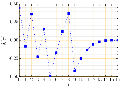
Figure 2: Phase shifts as a function of angular momentum channel number $l$ for the hard-sphere potential with $k_{f}R=11.17$. Note that channels with $l>12$ are effectively irrelevant.

The structure of the electron bubble as a spherical void of displaced ³He suggests the model of a short-range repulsive barrier preventing penetration of ³He into the bubble. The potential barrier, $V_{0}\approx 1\,\mbox{eV}$, is very large compared to typical quasiparticle kinetic energies, suggesting a reasonable model for the quasiparticle-ion potential is a single parameter hard-sphere potential parametrized by barrier radius $R$. The scattering phase shifts that define the quasiparticle-ion $t$-matrix for hard-sphere scattering are calculated in standard textbooks,Messiah (1958)

$$\tan\delta_{l}=\frac{j_{l}(k_{f}R)}{n_{l}(k_{f}R)}\,,$$ (9)

where $j_{l}(x)$ and $n_{l}(x)$ are order $l$ spherical Bessel functions of the first and second kind, respectively.

Figure (2) shows the set of phase shifts for a hard sphere with a ratio of radius to Fermi wavelength of $k_{f}R=11.17$. Note that for channels with $l\gtrsim k_{f}R$, the phase shift decreases rapidly to zero. The radius is determined by requiring the transport cross-section computed for the hard-sphere potential reproduce the measured normal-state ion mobility according to Eqs. (3), (8) and (9). At $P=0$ bar the Fermi wave number, $k_{f}=7.853\,\mbox{nm}^{-1}$, determines the Fermi momentum, $p_{f}=\hbar\,k_{f}$, and particle density, $n_{3}=k_{f}^{3}/3\pi^{2}$. Combined with the measured normal-state mobility, $\mu_{\text{N}}^{\text{exp}}=1.7\times 10^{-6}\,\mathrm{m^{2}/Vs}$,Ikegami et al. (2013) we obtain $k_{f}\,R=11.17$, smaller than the bubble radius determined by the surface tension and zero-point kinetic energy of the electron. For scattering of quasiparticles off the electron bubble this is the relevant measure of the size of the electron bubble. In what follows we develop the theory for the structure of the electron bubble in chiral superfluid ³He-A based on multiple scattering of Bogoliubov quasiparticles off the negative ion.

III Structure of an Electron Bubble in ³He-A

The structure of an electron bubble in ³He-A is much richer than that in normal ³He. However, multiple scattering channels of electon bubble are central in determining the spectrum of chiral Fermions confined near the electron bubble. Here we develop the theory for Bogoliubov quasiparticles scattering off an electron bubble embedded in superfluid ³He-A, and use the scattering theory to calculate the local spectrum of chiral Fermions bound to the electron bubble, as well as the mass current and angular momentum circulating the electron bubble. Our formulation parallels Refs. [Baym et al., 1977], [Salomaa et al., 1980], [Thuneberg et al., 1981] and [Salmelin and Salomaa, 1990]; however, we incorporate broken parity and time-reversal, in addition to broken $U(1)$ and $SO(3)$ symmetries, of the ground state of ³He-A in our formulation of the scattering of quasiparticles off electron bubbles.

Fermionic excitations of superfluid ³He-A are coherent superpositions of normal-state particles and holes described by four-component Bogoliubov-Nambu spinor wavefunctions, $\Psi(\mathbf{r})=(u_{\uparrow}(\mathbf{r}),u_{\downarrow}(\mathbf{r}),v_{\downarrow}(\mathbf{r}),v_{\uparrow}(\mathbf{r}))^{\mathrm{T}}$, that are solutions of Bogoliubov’s equations

$$\widehat{H}_{S}\Psi(\mathbf{r})=E\Psi(\mathbf{r}),\quad\widehat{H}_{S}=\begin{pmatrix}\hat{H}_{N}&\hat{\Delta}(\mathbf{p})\\ \hat{\Delta}^{\dagger}(\mathbf{p})&-\hat{H}_{N}\end{pmatrix}\,,$$ (10)

$$\hat{H}_{N}=(\frac{\mathbf{p}^{2}}{2m^{\ast}}-\mu)\,\mathbb{1}\,,\quad\hat{\Delta}({\mathbf{p}})=\sigma_{x}\Delta(\mathbf{p}_{x}+i\mathbf{p}_{y})/p_{f}\,,$$ (11)

where $\hat{\Delta}(\mathbf{p})$ is the mean-field pairing potential (order parameter) responsible for particle-hole coherence of the Fermionic excitations, and for branch conversion scattering between particle-like and hole-like Bogoliubov quasiparticles. Note that $\mathbf{p}=-i\hbar\nabla$, $\mathbb{1}$ is the unit matrix in spin space, and $\sigma_{x}$ is the Pauli matrix describing equal-spin pairing state (ESP) of Cooper pairs with spin projections $S_{x}=\pm 1$; equivalently, the Cooper pairs have zero spin projection along $\hat{\mathbf{z}}$. The chiral axis $\hat{\mathbf{l}}$ for A-phase Cooper pairs is also along $\hat{\mathbf{z}}$. Thus, the $4\times 4$ equation splits into a pair of two-component equations for $\Psi_{\uparrow}=(u_{\uparrow},0,0,v_{\uparrow})^{\mathrm{T}}$ and $\Psi_{\downarrow}=(0,u_{\downarrow},v_{\downarrow},0)^{\mathrm{T}}$.

III.1 Scattering States and Propagators

The scattering states are Bogoliubov quasiparticles in homogeneous ³He-A, i.e. far from the electron bubble, in which case the orbital part of the mean-field pairing potential can be expressed as $\Delta(\hat{\mathbf{k}}_{x}+i\hat{\mathbf{k}}_{y})=\Delta\sin\theta\,e^{+i\phi}$, where $\theta$ is the polar angle of the relative momentum of the Cooper pairs in momentum space and the azimuthal angle, $\phi$, is the phase of the Cooper pairs in momentum space that winds by $2\pi$ about the chiral axis, $\hat{\mathbf{l}}$. This phase winding plays a central role in the scattering of quasiparticles off the electron bubble embedded in ³He-A. The scattering states are eigenstates of momentum, $\mathbf{p}\mbox{$\displaystyle|\,\mathbf{k}\,\rangle$}=\hbar\mathbf{k}\,\mbox{$\displaystyle|\,\mathbf{k}\,\rangle$}$. There are four Bogoliubov quasiparticle states for each energy - particle-like and hole-like excitations each with two degenerate spin states. The Bogoliubov-Nambu spinors for the scattering states have the form

$$|\Psi_{1,\mathbf{k}\sigma}\rangle = \begin{pmatrix}u_{\mathbf{k}}\chi_{\sigma}\\ -v_{\mathbf{k}}^{\ast}\chi_{\bar{\sigma}}\end{pmatrix}\otimes|\mathbf{k}\rangle=|\Phi_{1,\mathbf{k}\sigma}\rangle\otimes|\mathbf{k}\rangle\,,$$ (12)

$$|\Psi_{2,\mathbf{k}\sigma}\rangle = \begin{pmatrix}v_{\mathbf{k}}\chi_{\sigma}\\ -u_{\mathbf{k}}^{\ast}\chi_{\bar{\sigma}}\end{pmatrix}\otimes|\mathbf{k}\rangle=|\Phi_{2,\mathbf{k}\sigma}\rangle\otimes|\mathbf{k}\rangle,$$ (13)

where the particle and hole amplitudes are given by

$$u_{\mathbf{k}}=\frac{1}{\sqrt{2}}\sqrt{1+\frac{\xi_{k}}{E_{\mathbf{k}}}}\,,\quad v_{\mathbf{k}}=\frac{1}{\sqrt{2}}\sqrt{1-\frac{\xi_{k}}{E_{\mathbf{k}}}}\,e^{i\phi}\,,$$ (14)

$$\langle\mathbf{r}|\mathbf{k}\rangle=e^{i\mathbf{k}\mathbf{r}}\,,\;\chi_{\uparrow}=\begin{pmatrix}1\\ 0\end{pmatrix}\,,\;\chi_{\downarrow}=\begin{pmatrix}0\\ 1\end{pmatrix}\,,\;\chi_{\bar{\uparrow}}=\chi_{\downarrow}\,,$$ (15)

where $E_{\mathbf{k}}=\sqrt{\xi_{\mathbf{k}}^{2}+|\Delta(\hat{\mathbf{k}})|^{2}}$ is the excitation energy for Bogoliubov quasiparticles. The spinors, $|\Psi_{1,\mathbf{k}\sigma}\rangle$, are the particle-like states with $\xi_{k}>0$ and group velocity $\nabla_{\mathbf{k}}E_{\mathbf{k}}>0$, while $|\Psi_{2,\mathbf{k}\sigma}\rangle$ are the hole-like states with $\xi_{k}<0$ and $\nabla_{\mathbf{k}}E_{\mathbf{k}}<0$. Note that the winding number of the Cooper pairs is imprinted as a relative phase between the particle- and hole like amplitudes in Eq. (14).

The causal propagator is the retarded Green’s function of Bogoliubov’s equations, $\left(\varepsilon\widehat{1}-\widehat{H}_{\text{S}}\right)\,\widehat{G}^{\text{R}}_{\text{S}}=\widehat{1}$, with $\varepsilon=E+i\eta$ ($\eta\rightarrow 0^{+}$), which for the bulk excitations in the homogeneous A-phase is given by

$$\widehat{G}^{\text{R}}_{\text{S}}(\mathbf{k},E)=\frac{1}{\varepsilon^{2}-E_{\mathbf{k}}^{2}}\begin{pmatrix}(\varepsilon+\xi_{k})\mathbb{1}&-\hat{\Delta}(\hat{\mathbf{k}})\\ -\hat{\Delta}^{\dagger}(\hat{\mathbf{k}})&(\varepsilon-\xi_{k})\mathbb{1}\end{pmatrix}\,.$$ (16)

Note that $\widehat{G}^{\text{R}}_{\text{S}}(\mathbf{k},E)$ is restricted to the low energy region of the Fermi surface where the normal-state is well described by long-lived quasiparticles. The corresponding Nambu matrix for the normal-state propagator,

$$\widehat{G}^{\text{R}}_{\text{N}}(\mathbf{k},E)=\begin{pmatrix}(\varepsilon-\xi_{k})^{-1}\mathbb{1}&0\\ 0&(\varepsilon+\xi_{k})^{-1}\mathbb{1}\end{pmatrix}\,,$$ (17)

includes both the particle- and hole propagators.

III.2 T matrix

The electron bubble introduces a strong, short-range potential that scatters Bogoliubov quasiparticles. The $t$-matrix is given by the Lippmann-Schwinger equation, which becomes a $4\times 4$ Nambu matrix whose elements define the transition amplitudes for scattering of Bogoliubov particles and holes, including branch conversion, i.e. Andreev scatteirng,

$$\widehat{T}_{\text{S}}=\widehat{V}+\widehat{V}\widehat{\mathcal{G}}^{\text{R}}_{\text{S}}\widehat{T}_{\text{S}}\,,\quad\mbox{where}\quad\widehat{V}=\begin{pmatrix}V(\mathbf{r})&0\\ 0&-V(\mathbf{r})\end{pmatrix}\,,$$ (18)

is the Nambu matrix for the ion potential, and $\widehat{\mathcal{G}}^{\text{R}}_{\text{S}}$ is the exact propagator in the presence of the local potential of the ion. For an ion with small cross-section on the scale of the size of Cooper pairs, we are justified in replacing $\widehat{\mathcal{G}}^{\text{R}}_{\text{S}}\rightarrow\widehat{G}^{\text{R}}_{\text{S}}$, i.e. the bulk propagator in the absence of the ion given by Eq. (16). We can use the corresponding Lippman-Schwinger equation for scattering of quasiparticles in the normal state to eliminate the ion potential $\hat{V}$ in favor of the normal-state $t$-matrix,Serene and Rainer (1983)

$$\widehat{T}_{S}=\widehat{T}_{N}+\widehat{T}_{N}\left(\widehat{G}_{S}^{R}-\widehat{G}_{N}^{R}\right)\widehat{T}_{S}\,.$$ (19)

The normal state $t$-matrix can be expressed in terms of the quasiparticle $t$-matrix, and has the diagonal form in Nambu space,

$$\widehat{T}_{\text{N}}(\hat{\mathbf{k}}^{\prime},\hat{\mathbf{k}})=\begin{pmatrix}t^{\text{R}}_{\text{N}}(\hat{\mathbf{k}}^{\prime},\hat{\mathbf{k}})\mathbb{1}&0\\ 0&-\left[t^{\text{R}}_{\text{N}}(-\hat{\mathbf{k}}^{\prime},-\hat{\mathbf{k}})\mathbb{1}\right]^{\dagger}\end{pmatrix}\,.$$ (20)

The ground state of ³He-A breaks rotational symmetry, but preserves axial rotations combined with a compensating gauge transformation. Thus, scattering of quasiparticles off the electron bubble in ³He-A no longer separates into angular momentum channels with a precise $l$. However, the projection of the angular mometum, labelled by $m$, is conserved for non-branch conversion scattering, and changes by one unit of angular momentum for branch conversion scattering. Thus, in reducing the $t$-matrix for the scattering of Bogoliubov quasiparticles in ³He-A, it is convenient to rewrite Eq. (6) as an expansion in azimuthal harmonics by using the addition theorem to express the Legendre functions in terms of the spherical harmonics.Mathews and Walker (1965) We then change the order of the summations over $l$ and $m$,

$$t_{N}(\hat{\mathbf{k}}^{\prime},\hat{\mathbf{k}}) = -\frac{1}{\pi N_{F}}\sum_{m=-\infty}^{\infty}t_{N}^{m}(u^{\prime},u)e^{-im(\phi^{\prime}-\phi)},$$ (21)

$$t_{N}^{m}(u^{\prime},u) = 4\pi\sum_{l=|m|}^{\infty}e^{i\delta_{l}}\sin\delta_{l}\,\Theta_{l}^{m}(u^{\prime})\Theta_{l}^{m}(u),$$

where $(\theta,\phi)$ [$(\theta^{\prime},\phi^{\prime})$] are spherical coordinates of $\hat{\mathbf{k}}$ [$\hat{\mathbf{k}}^{\prime}$] in momentum space, with $u\equiv\cos\theta$ and $u^{\prime}\equiv\cos\theta^{\prime}$. The functions $\Theta_{l}^{m}(\cos\theta)$ are spherical harmonics with the phase winding removed, i.e. $Y_{l}^{m}(\theta,\phi)=\Theta_{l}^{m}(\cos\theta)\,e^{im\phi}$.

For elastic scattering of Bogoliubov quasiparticles we can reduce Eq. (19) to a linear integral equation with $\widehat{T}^{\text{R}}_{\text{N}}(\hat{\mathbf{k}}^{\prime},\hat{\mathbf{k}})$ as the source term,

$$\widehat{T}^{\text{R}}_{\text{S}}(\hat{\mathbf{k}}^{\prime},\hat{\mathbf{k}};E)=\widehat{T}^{\text{R}}_{\text{N}}(\hat{\mathbf{k}}^{\prime},\hat{\mathbf{k}})+N_{f}\negthickspace\int\frac{d\Omega_{\mathbf{k}^{\prime\prime}}}{4\pi}\times\qquad\qquad\quad$$

$$\widehat{T}^{\text{R}}_{\text{N}}(\hat{\mathbf{k}}^{\prime},\hat{\mathbf{k}}^{\prime\prime})[\widehat{g}^{\text{R}}_{\text{S}}(\hat{\mathbf{k}}^{\prime\prime},E)-\widehat{g}^{\text{R}}_{\text{N}}(\hat{\mathbf{k}}^{\prime\prime},E)]\widehat{T}^{\text{R}}_{\text{S}}(\hat{\mathbf{k}}^{\prime\prime},\hat{\mathbf{k}};E)\,,$$ (22)

where the propagators in Eq. (III.2) are confined to a narrow shell of energies and momenta near the Fermi surface and evaluated in the quasiclassical approximation,

$$\widehat{g}^{\text{R}}_{\text{S}}(\hat{\mathbf{k}}^{\prime\prime},E)=-\frac{\pi}{\sqrt{|\Delta(\hat{\mathbf{k}})|^{2}-\varepsilon^{2}}}\begin{pmatrix}\varepsilon\mathbb{1}&-\hat{\Delta}(\hat{\mathbf{k}})\\ -\hat{\Delta}^{\dagger}(\hat{\mathbf{k}})&\varepsilon\mathbb{1}\end{pmatrix}\,.$$ (23)

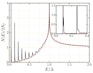
Figure 3: (Color online) Local quasiparticle density of states around an electron bubble in superfluid ³He-A at distance $r=30\,k_{f}^{-1}$ from the center of the bubble, and in the equitorial plane, i.e. polar angle $\vartheta=\pi/2$ relative to the chiral axis. The bubble is described as a hard sphere with radius $R=11.17\,k_{f}^{-1}$. The inset shows two low-energy resonances with internal structure in their spectral density.

The corresponding normal-state quasiclassical propagator is $\widehat{g}^{\text{R}}_{\text{N}}(\mathbf{k},E)=-i\pi\widehat{1}$. For scattering off an electron bubble in ³He-A the quasiclassical $t$-matrix reduces to a set of $4\times 4$ matrix equations for scattering amplitudes, $t^{m}_{a}$ for Nambu components, $a=1,2,3,4$, for each angular momentum quantum number, $m\in\{0\,\pm 1,\pm 2,\ldots\}$. In particular, we parametrize $\widehat{T}^{\text{R}}_{\text{S}}$ as

$$\widehat{T}^{\text{R}}_{\text{S}}=\negthickspace\begin{pmatrix}t_{1}(\hat{\mathbf{k}}^{\prime},\hat{\mathbf{k}};E)\mathbb{1}&t_{2}(\hat{\mathbf{k}}^{\prime},-\hat{\mathbf{k}};E)\sigma_{x}\cr t_{3}(-\hat{\mathbf{k}}^{\prime},\hat{\mathbf{k};E})\sigma_{x}&t_{4}(-\hat{\mathbf{k}}^{\prime},-\hat{\mathbf{k}};E)\mathbb{1}\end{pmatrix}=\negthickspace\frac{-1}{\pi N_{F}}\sum\limits_{m=-\infty}^{\infty}\negthickspace e^{-im(\phi^{\prime}-\phi)}\negthickspace\begin{pmatrix}t_{1}^{m}(u^{\prime},u)\mathbb{1}&(-1)^{m}e^{i\phi^{\prime}}t_{2}^{m}(u^{\prime},-u)\sigma_{x}\cr(-1)^{m+1}e^{-i\phi^{\prime}}t_{3}^{m}(-u^{\prime},u)\sigma_{x}&t_{4}^{m}(-u^{\prime},-u)\mathbb{1}\end{pmatrix}\,.$$ (24)

The prefactors $(-1)^{m}$ in Eq. (24) reflect the sign changes for branch conversion scattering, i.e. $\hat{\mathbf{k}}\rightarrow-\hat{\mathbf{k}}$ is equivalent to $(\theta\rightarrow\pi-\theta,\phi\rightarrow\pi+\phi)$. The factors of $\exp(\pm i\phi^{\prime})$ in the off-diagonal terms reflect the phase winding of the order parameter. This parametrization reduces the matrix integral equation to a set of coupled one-dimensional integral equations for ${t}^{m}_{a}(u^{\prime},u)$,

$${t}_{1}^{m}(u^{\prime},u)=t_{N}^{m}(u^{\prime},u)+\int\limits_{-1}^{1}\frac{du^{\prime\prime}}{2}t_{N}^{m}(u^{\prime},u^{\prime\prime})\left[\mathfrak{G}^{\text{R}}(\hat{\mathbf{k}}^{\prime\prime},\varepsilon){t}_{1}^{m}(u^{\prime\prime},u)+(-1)^{m}e^{-i\phi^{\prime\prime}}\mathfrak{F}^{\text{R}}(\hat{\mathbf{k}}^{\prime\prime},\varepsilon){t}_{3}^{m}(-u^{\prime\prime},u)\right]\,,$$ (25)

$${t}_{3}^{m}(-u^{\prime},u)=-\int\limits_{-1}^{1}\frac{du^{\prime\prime}}{2}t_{N}^{m+1}(u^{\prime},u^{\prime\prime})^{*}\left[\mathfrak{G}^{\text{R}}(\hat{\mathbf{k}}^{\prime\prime},\varepsilon){t}_{3}^{m}(-u^{\prime\prime},u)+(-1)^{m}e^{i\phi^{\prime\prime}}\mathfrak{F}^{\text{R}}(\hat{\mathbf{k}}^{\prime\prime},\varepsilon)^{*}{t}_{1}^{m}(u^{\prime\prime},u)\right]\,,$$ (26)

$${t}_{2}^{m}(u^{\prime},-u)=\int\limits_{-1}^{1}\frac{du^{\prime\prime}}{2}t_{N}^{m-1}(u^{\prime},u^{\prime\prime})\left[\mathfrak{G}^{\text{R}}(\hat{\mathbf{k}}^{\prime\prime},\varepsilon){t}_{2}^{m}(u^{\prime\prime},-u)+(-1)^{m+1}e^{-i\phi^{\prime\prime}}\mathfrak{F}^{\text{R}}(\hat{\mathbf{k}}^{\prime\prime},\varepsilon){t}_{4}^{m}(-u^{\prime\prime},-u)\right]\,,$$ (27)

$${t}_{4}^{m}(-u^{\prime},-u)=-t_{N}^{m}(u^{\prime},u)^{*}-\int\limits_{-1}^{1}\frac{du^{\prime\prime}}{2}t_{N}^{m}(u^{\prime},u^{\prime\prime})^{*}\left[\mathfrak{G}^{\text{R}}(\hat{\mathbf{k}}^{\prime\prime},\varepsilon){t}_{4}^{m}(-u^{\prime\prime},-u)+(-1)^{m+1}e^{i\phi^{\prime\prime}}\mathfrak{F}^{\text{R}}(\hat{\mathbf{k}}^{\prime\prime},\varepsilon)^{*}{t}_{2}^{m}(u^{\prime\prime},-u)\right]\,,$$ (28)

where

$$\mathfrak{G}^{\text{R}}(\hat{\mathbf{k}},\varepsilon) = \frac{\varepsilon}{\sqrt{|\Delta(\hat{\mathbf{k}})|^{2}-\varepsilon^{2}}}-i\,,$$ (29)

$$\mathfrak{F}^{\text{R}}(\hat{\mathbf{k}},\varepsilon) = \frac{\Delta(\hat{\mathbf{k}})}{\sqrt{|\Delta(\hat{\mathbf{k}})|^{2}-\varepsilon^{2}}}\,.$$ (30)

Note that ${t}_{1}^{m}(u^{\prime},u)$ is the scattering amplitude for quasiparticle excitations with angular momentum projection $m$, while $t_{4}^{m}(u^{\prime},u)$ is the corresponding quasi-hole amplitude. Branch conversion scattering, generated by the anomalous propagator, $\mathfrak{F}^{\text{R}}(\hat{\mathbf{k}},\varepsilon)$, is given by the amplitudes $t_{2}^{m}(u^{\prime},-u)$ (hole $\rightarrow$ particle) and $t_{3}^{m}(-u^{\prime},u)$ (particle $\rightarrow$ hole). Multiple scattering couples these amplitudes in pairs, $\{{t}_{1}^{m},{t}_{3}^{m}\}$ and $\{{t}_{2}^{m},{t}_{4}^{m}\}$ as indicated in Eqs. (25-26) and Eqs. (27-28). The sets of equations are solved numerically. In Sec. (IV) the solution to the $t$-matrix is used to calculate the differential cross-section for the scattering of Bogoliubov quasiparticles off the electron bubble, and from that the forces on electron bubbles moving in response to an external electric field.

III.3 Local Density of States

We first use the $t$-matrix to calculate the spectrum of chiral Fermions bound to the electron bubble. The asymmetry in the spectrum with respect to the orbital quantum number is responsible for the ground state current and angular momentum bound to the electron bubble. The Nambu Green’s function determines the local density of states,

$$N(\mathbf{r},E)=-\frac{1}{2\pi}\mathrm{Im}\left\{\mathrm{Tr}\left[\widehat{\mathcal{G}}^{\text{R}}_{\text{S}}(\mathbf{r},\mathbf{r};E)\right]\right\}\,,$$ (31)

where the trace is over both particle-hole and spin space, and $\widehat{\mathcal{G}}^{\text{R}}_{\text{S}}(\mathbf{r}^{\prime},\mathbf{r};E)$ is the retarded Green’s function in the presence of an electron bubble. It is convenient to express $\widehat{\mathcal{G}}^{\text{R}}_{\text{S}}(\mathbf{r}^{\prime},\mathbf{r};E)$ in momentum space,

$$\mathcal{G}^{\text{R}}_{\text{S}}(\mathbf{r}^{\prime},\mathbf{r};E)=\negthickspace\int\frac{d^{3}k}{(2\pi)^{3}}\negthickspace\int\frac{d^{3}k^{\prime}}{(2\pi)^{3}}e^{i(\mathbf{k}^{\prime}\cdot\mathbf{r}^{\prime}-\mathbf{k}\cdot\mathbf{r})}\mathcal{G}^{\text{R}}_{\text{S}}(\mathbf{k}^{\prime},\mathbf{k};E)\,.$$ (32)

The low-energy Nambu Green’s function for quasiparticles and pairs in the presence of the ion potential can be expressed in terms of the bulk propagator and the quasiparticle-ion $t$-matrix,

$$\widehat{\mathcal{G}}^{\text{R}}_{\text{S}}(\mathbf{k}^{\prime},\mathbf{k};E) = (2\pi)^{3}\delta(\mathbf{k}^{\prime}-\mathbf{k})\,\widehat{G}^{\text{R}}_{\text{S}}(\mathbf{k},E)$$ (33)

$$+ \widehat{G}^{\text{R}}_{\text{S}}(\mathbf{k}^{\prime},E)\widehat{T}^{\text{R}}_{\text{S}}(\mathbf{k}^{\prime},\mathbf{k};E)\widehat{G}^{\text{R}}_{\text{S}}(\mathbf{k},E)\,.$$

For energies $|E|\ll E_{f}$ we can evaluate the $t$-matrix and propagators in the quasiclassical approximation and obtain an explicit expression for the local density of states (LDOS).

Figure (3) shows the local density of states calculated at the position, $r=30\,k_{f}^{-1}$ and $\vartheta=\pi/2$, i.e. approximately $19$ Fermi wavelengths from the surface of the electron bubble. The bulk density of states is shown as the dashed line. A van Hove singularity occurs at the maximum gap in the bulk excitation spectrum, while the low-energy spectrum results from the nodal quasiparticles near $\theta=0,\pi$. Multiple scattering, both potential and branch conversion, by the ion and the chiral order parameter generates Andreev bound states indexed by the angular momentum channel, $m$, and linear momentum, $p_{z}=p_{f}\cos\theta$. The bound states are broadened into low-energy bands by integration over $p_{z}$, and then into resonances by hybridization with the continuum of nodal quasiparticles. There are $l_{\text{max}}\approx k_{f}R\approx 12$ sub-gap resonances shown in Fig. (3).

More detailed spectral information is obtained by resolving the LDOS in angular momentum channels. The reduction of the $t$-matrix as a sum over amplitudes with well defined angular momentum projection implies a similar chiral decomposition of the LDOS,

$$N(\mathbf{r},E)=N_{0}(E)+\sum_{m=-\infty}^{\infty}\delta N_{m}(\mathbf{r},E)\,,$$ (34)

where $N_{0}(E)$ is the bulk density of states in superfluid $\mathrm{{}^{3}He-A}$

$$N_{0}(E)=N_{F}\frac{|E|}{\Delta}\ln\left|\frac{|E|+\Delta}{|E|-\Delta}\right|\,,$$ (35)

and $\delta N_{m}(\mathbf{r},E)$, obtained from Eqs. (31)-(33) with the solutions of Eqs. (25)-(28), is given by

$$\delta N_{m}(\mathbf{r},E)\negthickspace = \negthickspace 4\pi^{2}N_{f}\,\mathrm{Im}\Biggl{\{}\negthickspace\sum_{l,l^{\prime}=|m|}^{\infty}\Theta_{l^{\prime}}^{m}(v)\Theta_{l}^{m}(v)\negthickspace\int_{-1}^{1}\negthickspace du^{\prime}\Theta_{l^{\prime}}^{m}(u^{\prime})e^{-\sqrt{\Delta^{2}(1-u^{\prime 2})-\varepsilon^{2}}\frac{r}{\hbar v_{f}}}\int_{-1}^{1}\negthickspace du\,\Theta_{l}^{m}(u)e^{-\sqrt{\Delta^{2}(1-u^{2})-\varepsilon^{2}}\frac{r}{\hbar v_{f}}}K_{l^{\prime}l}^{m}(u^{\prime},u,\varepsilon)\negthickspace\Biggr{\}},$$ (36)

where $u=\cos\theta$ and $u^{\prime}=\cos\theta^{\prime}$ in momentum space, $\mathbf{r}=(r,\vartheta,\varphi)$ is the spatial coordiate in spherical coordinates with $v=\cos\vartheta$, and the matrix elements, $K_{ll^{\prime}}^{m}$, are given in terms of spherical Bessel functions, the intermediate propagator and the elements of the $t$-matrix (see App. B for details leading to Eq. 37),

$$K_{l^{\prime}l}^{m}(u^{\prime},u,\varepsilon) =i^{l^{\prime}-l}\Biggl{\{}\frac{j_{l^{\prime}}(k_{F}r)j_{l}(k_{F}r)}{\sqrt{\Delta^{2}(1-u^{\prime 2})-\varepsilon^{2}}\sqrt{\Delta^{2}(1-u^{2})-\varepsilon^{2}}}\Bigl{[}\Delta^{2}\sqrt{1-u^{\prime 2}}\sqrt{1-u^{2}}(t^{m-1}_{1}+t^{m+1}_{4})+\varepsilon^{2}(t^{m}_{1}+t^{m}_{4})$$

$$+(-1)^{m}\Delta\varepsilon\sqrt{1-u^{\prime 2}}(t^{m}_{3}-t^{m}_{2})+(-1)^{m}\Delta\varepsilon\sqrt{1-u^{2}}(t^{m+1}_{2}-t^{m-1}_{3})\Bigr{]}+n_{l^{\prime}}(k_{F}r)n_{l}(k_{F}r)(t^{m}_{1}+t^{m}_{4})$$

$$-\frac{j_{l^{\prime}}(k_{F}r)n_{l}(k_{F}r)}{\sqrt{\Delta^{2}(1-u^{\prime 2})-\varepsilon^{2}}}\Bigl{[}\varepsilon(t^{m}_{1}-t^{m}_{4})+(-1)^{m}\Delta\sqrt{1-u^{\prime 2}}(t^{m}_{2}+t^{m}_{3})\Bigr{]}$$

$$-\frac{n_{l^{\prime}}(k_{F}r)j_{l}(k_{F}r)}{\sqrt{\Delta^{2}(1-u^{2})-\varepsilon^{2}}}\Bigl{[}\varepsilon(t^{m}_{1}-t^{m}_{4})+(-1)^{m}\Delta\sqrt{1-u^{2}}(t^{m+1}_{2}+t^{m-1}_{3})\Bigr{]}\Biggr{\}}\,\equiv\,i^{l^{\prime}-l}\,\kappa^{m}_{l^{\prime}l}(u^{\prime},u,\varepsilon)\,.$$ (37)

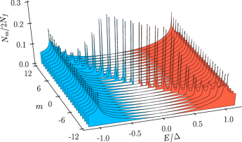
Figure 4: (Color online) The LDOS resolved into orbital angular momentum components labelled by $m$ as defined by Eq. 39. $N_{m}(\mathbf{r},E)$ represents a discrete spectrum of Weyl Fermions bound to the electron bubble, plus hybridization with the nodal quasiparticles. Note the double degeneracy of each sub-gap energy level.

The BTRP symmetry of the order parameter $\Delta(\hat{\mathbf{k}})$ implies that Andreev scattering involves transitions between states with $m$ and $m\pm 1$. This mixing of channels is clarified by resolving the LDOS in the orbital angular momentum index $m$. Here it is worth noting that the sum over $m$ in Eq. (34), while formally extending to $\pm\infty$, is in practice restricted to $|m|\leq l_{\text{max}}\approx k_{f}R\approx 12$ [see Fig. (2)]. Thus, we resolve the LDOS as

$$N(\mathbf{r},E)=\sum_{m=-l_{\text{max}}}^{l_{\text{max}}}N_{m}(\mathbf{r},E)\,,$$ (38)

$$N_{m}(\mathbf{r},E)=\frac{1}{2l_{\text{max}}+1}N_{0}(E)+\delta N_{m}(\mathbf{r},E)\,.$$ (39)

Equation (36) contains exponential factors varying on the coherence length scale, as well as fast oscillations, encoded in the spherical Bessel functions, varying on the scale of the Fermi wavelength. In Figs. (3) and (4) we averaged $\delta N_{m}(\mathbf{r},E)$ over a Fermi wavelength,

$$\delta N_{m}^{\mathrm{qc}}(\mathbf{r},E)=\frac{1}{\lambda_{f}}\int_{r-\lambda_{f}/2}^{r+\lambda_{f}/2}\delta N_{m}(\mathbf{r},E)\,,$$ (40)

to eliminate the atomic scale oscillations.

In Fig. (4) we plot the angular-momentum-resolved LDOS, $N_{m}(\mathbf{r},E)$, as a function of energy. Note that the bound states appear in neighboring pairs of $m$-channels, and that, except for the two states with $m=0$, the bound states for $E\geq 0$ ($E\leq 0$) occur only for channels with $m>0$ ($m<0$), the key feature of a Weyl spectrum of chiral Fermions.

III.4 Bubble Edge Currents

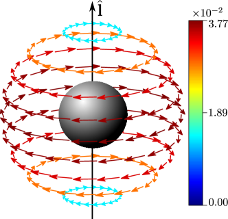
Figure 5: (Color online) Current density $\mathbf{j}(\mathbf{r})$ in units of $N_{f}v_{f}k_{B}T_{c}$ calculated at distance $k_{F}r=30.0$ from the bubble center. We used the hard sphere model with $k_{F}R=11.17$, shown in gray. The chiral axis $\hat{\mathbf{l}}$ determines the direction of Cooper pair angular momentum. The temperature is taken as $T=0.5T_{c}$.

The spectrum of chiral Fermions bound to the electron bubble in ³He-A is responsible for the ground state current circulating the bubble, the mesoscopic realization of ground-state edge currents on a macroscopic boundary of a superfluid ³He-A film. The current circulating an electron bubble is calculated from the Fermi distribution and the full retarded and advanced Green’s functions, $\widehat{\mathcal{G}}^{\text{R,A}}_{\text{S}}(\mathbf{r}^{\prime},\mathbf{r};E)$, based on Eqs. (33), (16), (24) and (25)-(28),

$$\mathbf{j}(\mathbf{r}) = \frac{\hbar}{4}\negthickspace\int\negthickspace\frac{dE}{2\pi}(f(E)-\genfrac{}{}{}{1}{1}{2})$$ (41)

$$\times (\boldsymbol{\nabla}_{\mathbf{r}^{\prime}}\negthickspace-\negthickspace\boldsymbol{\nabla}_{\mathbf{r}})\mathrm{Tr}\,\left[\widehat{\mathcal{G}}^{\text{R}}_{\text{S}}(\mathbf{r}^{\prime},\mathbf{r};E)-\widehat{\mathcal{G}}^{\text{A}}_{\text{S}}(\mathbf{r}^{\prime},\mathbf{r};E)\right]_{\mathbf{r}=\mathbf{r}^{\prime}}\negthickspace\negthickspace.$$

The current circulating the electron bubble comes from the $t$-matrix term in Eq. (33). To calculate the current it is more efficient to recast Eq. (41) in terms of the Matsubara Green’s function,

$$\mathbf{j}(\mathbf{r})=\frac{\hbar}{4i}k_{\text{B}}T\sum_{n=-\infty}^{\infty}\left[(\boldsymbol{\nabla}_{\mathbf{r}^{\prime}}-\boldsymbol{\nabla}_{\mathbf{r}})\mathrm{Tr}\,\widehat{\mathcal{G}}^{\text{M}}(\mathbf{r}^{\prime},\mathbf{r};\epsilon_{n})\right]_{\mathbf{r}=\mathbf{r}^{\prime}}\,,$$ (42)

where $\epsilon_{n}=(2n+1)\pi k_{\text{B}}T$ are Matsubara frequencies, and the Matsubara Green’s function is related to the retarded and advanced Green’s functions by analytic continuation,Abrikosov et al. (1965)

$$\mathcal{G}^{\text{R(A)}}_{\text{S}}(\mathbf{r}^{\prime},\mathbf{r},E)=\mathcal{G}^{\text{M}}_{\text{S}}(\mathbf{r}^{\prime},\mathbf{r},\epsilon_{n})\Bigr{|}_{i\epsilon_{n}\rightarrow E\pm i0},\;\mbox{for $\varepsilon_{n}\gtrless 0$}\,.$$ (43)

After Fourier-transforming Eq. (42) we obtain

$$\mathbf{j}(\mathbf{r})\negthickspace=\negthickspace\frac{\hbar}{4}k_{\text{B}}T\negthickspace\sum_{n=-\infty}^{\infty}\negthickspace\left[\sum_{\mathbf{k},\mathbf{k}^{\prime}}(\mathbf{k}^{\prime}+\mathbf{k})\,e^{i(\mathbf{k}^{\prime}-\mathbf{k})\cdot\mathbf{r}}\,\mathrm{Tr}\,\widehat{\mathcal{G}}^{\text{M}}(\mathbf{k}^{\prime},\mathbf{k};\epsilon_{n})\right]\,.$$ (44)

We calculate the current from the propagator, $\widehat{\mathcal{G}}^{\text{M}}_{\text{S}}(\mathbf{k}^{\prime},\mathbf{k};\epsilon_{n})$, by analityic contiuation of the $t$-matrix, $\widehat{T}^{\text{M}}_{\text{S}}(\mathbf{r}^{\prime},\mathbf{r};\epsilon_{n})$, which satisfies the system of Eqs. (25)-(28), with $\varepsilon\rightarrow i\epsilon_{n}$. The real-valuedness of the current is ensured by the symmetry of the Nambu-Matsubara Green’s function,

$$\widehat{\mathcal{G}}^{\text{M}}_{\text{S}}(\mathbf{k},\mathbf{k}^{\prime},-\epsilon_{n})=\left[\widehat{\mathcal{G}}^{\text{M}}_{\text{S}}(\mathbf{k},\mathbf{k}^{\prime},\epsilon_{n})\right]^{\dagger}\,,$$ (45)

which also allows us to express the result for the current as a sum over $\varepsilon_{n}>0$. The current is purely azimuthal, $\mathbf{j}(r,\vartheta,\phi)=j_{\phi}(r,\vartheta)\mathbf{e}_{\phi}$ (see App. (C)), with $j_{\phi}(r,\vartheta)$ given by

$$j_{\phi}(r,\vartheta) = -8\pi^{3}v_{f}N_{f}k_{B}T\,\sum_{n=0}^{\infty}\sum_{m=-\infty}^{\infty}\sum_{l^{\prime}=|m-1|}^{\infty}\sum_{l=|m|}^{\infty}J_{l^{\prime}l}^{m}\,\,\Theta_{l^{\prime}}^{m-1}(\cos\vartheta)\Theta_{l}^{m}(\cos\vartheta)\,,$$ (46)

$$J_{l^{\prime}l}^{m} \equiv \mathrm{Im}\left[i^{l^{\prime}-l}\right]\int_{-1}^{1}du^{\prime}\int_{-1}^{1}du\sqrt{1-u^{\prime 2}}\,\Theta_{l^{\prime}}^{m-1}(u^{\prime})e^{-\sqrt{\Delta^{2}(1-u^{\prime 2})+\epsilon_{n}^{2}}{\frac{\text{\normalsize$r$}}{\text{\normalsize$\hbar v_{f}$}}}}\Theta_{l}^{m}(u)e^{-\sqrt{\Delta^{2}(1-u^{2})+\epsilon_{n}^{2}}{\frac{\text{\normalsize$r$}}{\text{\normalsize$\hbar v_{f}$}}}}\mathrm{Re}\left[\kappa_{l^{\prime}l}^{m}(u^{\prime},u,i\epsilon_{n})\right]\,,$$ (47)

where the functions $\kappa_{l^{\prime}l}^{m}(u^{\prime},u,i\varepsilon_{n})$ are analytically continued to the Matsubara energies, $\varepsilon\rightarrow i\varepsilon_{n}$.

The current circulating the electron bubble is shown in Fig. (5) for angular positions on a sphere of radius $r=30\,k_{f}^{-1}\approx 3.82\,\mbox{nm}$, i.e. in the near vicinity of the electron bubble with hard sphere radius $R=11.17\,k_{f}^{-1}\approx 1.42\,\mbox{nm}$. Note that the axial current flow is opposite to the chiralty of the ground state Cooper pairs for all polar angles, and the current vanishes in the direction of the chiral axis, i.e. along the nodal points of the order parameter. The direction of the current flow about the bubble agrees with our expectation based on the direction of the edge current for a macroscopic hole, i.e. for a locally translational invariant boundary, as illustrated in Fig. (1).

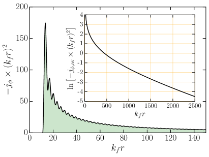
Figure 6: (Color online) Radial dependence of the current density $j_{\phi}(r,\vartheta)$ for $\vartheta=\pi/2$, in units of $v_{f}N_{f}k_{B}T_{c}$, calculated for the electron bubble with hard sphere radius of $k_{f}R=11.17$ and temperature $T=0.5T_{c}$. The current develops sharply from the bubble radius, then decays rapidly for $r>R$. Quantum oscillations on the Fermi wavelength scale are evident at short distances. Inset: The current decays exponentially, $j_{\phi,\text{av}}\sim-e^{-r/\xi_{0}}/(k_{f}r)^{2}$, at distances greater than the coherence length, $\xi_{0}=608.7\,k_{f}^{-1}$; $j_{\phi,\text{av}}$ is the quasiclassical envelope obtained by averaging $j_{\phi}(r)$ over a Fermi wavelength as in Eq. 40.

The current density varies with radial distance from the edge of the electron bubble as shown in Fig. (6). Note that the current is large on mesoscopic length scales, $R<r\ll\xi_{0}$, and decays very rapidly for $k_{f}r\gtrsim 15$. Quantum oscillations on the scale of the Fermi wavelength are evident at short distances. For $r\gtrsim\xi_{0}$ the current density is small and continues to decay exponentially on the scale of the coherence length as shown in the inset of Fig. (6).

The confinement of the current near the edge of the bubble endows the electron bubble with an angular momentum obtained by integrating the angular momentum density from the circulating edge current, $\mathbf{L}=\int d^{3}r\,\mathbf{r}\times\mathbf{j}(\mathbf{r})=L_{z}\,\mathbf{e}_{z}$,

$$L_{z}=2\pi\int_{R}^{\infty}r^{2}dr\int_{-1}^{+1}d(\cos\vartheta)\,(r\sin\vartheta)\,j_{\phi}(r,\vartheta)\,,$$ (48)

where the lower limit is set by the vanishing of $j_{\phi}$ for $r\leq R$.

Recalling our result for the angular momentum generated by edge currents circulating a macroscopic hole of radius $R\gg\xi_{0}$ in a thin ³He-A film, we express the angular momentum of the electron bubble edge currents in similar units, i.e.

$$L_{z} = -\mathfrak{f}\,\left(\frac{N_{\text{bubble}}}{2}\right)\,\hbar\,,$$ (49)

$$N_{\text{bubble}} = \genfrac{}{}{}{1}{4}{9\pi}(k_{f}R)^{3}\approx 197\,,$$ (50)

where $N_{\text{bubble}}$ is the number of ³He atoms excluded from the electron bubble. The negative sign reflects the fact that the angular momentum of the chiral currents is opposite to the chirality of the Cooper pairs. Numerical integration of Eq. (48) gives $\mathfrak{f}=1.3$, remarkably close to the prediction based on the volume of a macroscopic hole ($R\gg\xi_{0}$) in a ³He-A film, even though the electron bubble is in the limit, $R\ll\xi_{0}$. Indeed the angular momentum calculated for mesoscopic hard sphere bubbles, scaled in units of $-(N_{\text{bubble}}/2)\hbar$, is shown in Fig. (7) to rapidly approach the macroscopic scaling result for $k_{f}R\gg 1$. Already at $k_{f}R=25$, which corresponds to $R/\xi_{0}\approx 0.04$, the deviation from the macroscopic scaling result is only $\approx 7\%$. The inset of Fig. (7) shows the temperature dependence of $L_{z}$ for the electron bubble, scaling as $|\Delta(T)|^{2}\sim|T-T_{c}|$ in the Ginzburg-Landau (GL) limit.

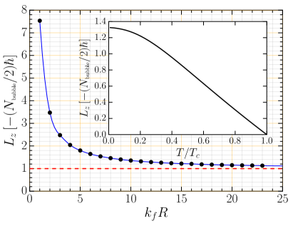
Figure 7: (Color online) Angular momentum of hard sphere “bubbles” embedded in ³He-A as a function of hard sphere radius, $k_{f}R$. For an electron bubble, $k_{f}R=11.17$. In the macroscopic limit, $R\gg\xi_{0}$ (red dashed line), $L_{z}$ scales to $L_{z}^{\infty}=-(N_{\text{bubble}}/2)\,\hbar$ Inset: Temperature dependence of $L_{z}$ for the electron bubble.

IV Electron mobility in ³He-A

Application of a d.c. electric field accelerates the electron bubble to a terminal velocity $\mathbf{v}=\overset{\text{\scriptsize$\leftrightarrow$}}{\mu}\cdot\mathbf{E}$, where the mobility, $\overset{\text{\scriptsize$\leftrightarrow$}}{\mu}$, is determined by forces acting on the moving electron bubble. At finite temperature the mobility is limited by the “wind” of thermal quasiparticles scattering off the moving electron bubble. In the normal phase of ³He the scattering rate is sufficiently large that recoil of the ion is suppressed, implying elastic scattering and a normal-state mobility that is temperature independent.Josephson and Lekner (1969); Anderson et al. (1968) Below $T_{c}$ the opening of a gap in the excitation spectrum leads to a rapid increase in the mobility.Bowley (1977) Experimentally, the mobility increases faster than expected based just on the reduction in the number of thermal quasiparticles. Baym et al. Baym et al. (1977) showed that in the superfluid B-phase the transport cross-section is also reduced by resonant forward scattering of Bogoliubov quasiparticles off the electron bubble. Their theory provides quantitative agreement with measurements of the mobility in ³He-B in the temperature regime near $T_{c}$.Ahonen et al. (1976)

For the chiral A phase these two basic features also operate. However, superfluid ³He-A has an anisotropic excitation gap that vanishes for momenta $\mathbf{k}||\pm\hat{\mathbf{l}}$ and is maximal for momenta $\mathbf{k}\perp\hat{\mathbf{l}}$. Thus, an electron bubble will experience a stronger drag force for $\mathbf{v}||\pm\hat{\mathbf{l}}$ compared to $\mathbf{v}\perp\hat{\mathbf{l}}$, i.e. $\mu_{||}<\mu_{\perp}$. Indeed the anisotropy of the negative ion mobility was calculated by extending the scattering theory for the B-phase by Baym et al.Baym et al. (1977) to scattering by an ion in ³He-A,Salomaa et al. (1980); Salmelin and Salomaa (1987) and measurements of the mobility anisotropy, $\mu_{\perp}-\mu_{||}$ were made via pulse-shape, time-of-flight experiments on vortex textures of superfluid ³He-A.Simola et al. (1986) Note that the drag force on the electron bubble is insensitive to the direction of the chiral axis, i.e. the drag force for $+\mathbf{E}||\hat{\mathbf{l}}$ and $-\mathbf{E}||\hat{\mathbf{l}}$ are the same.

The chiral axis is a reflection of broken time-reversal symmetry ($\mathrm{T}$) and broken mirror symmetry ($\Pi$) in a plane containing the chiral axis $\hat{\mathbf{l}}$. The generalization of the mobility for the isotropic B-phase to ³He-A with chiral axis $\hat{\mathbf{l}}||\hat{\mathbf{z}}$ is a mobility tensor, $\mu_{ij}$ with $i,j\in\{x,y.z\}$; thus, $v_{i}=\mu_{ij}E_{j}$, where the components are all real. Uniaxial rotation symmetry restricts the elements of the mobility tensor to $\mu_{xx}=\mu_{yy}\equiv\mu_{\perp}$, $\mu_{zz}\equiv\mu_{||}$, and $\mu_{xy}=-\mu_{yx}$; all other components vanish. Thus, the electron mobility tensor for ³He-A has the form

$$\mu_{ij}=\mu_{\perp}(\delta_{ij}-\hat{\mathbf{l}}_{i}\hat{\mathbf{l}}_{j})+\mu_{||}\hat{\mathbf{l}}_{i}\hat{\mathbf{l}}_{j}+\mu_{xy}\epsilon_{ijk}\hat{\mathbf{l}}_{k}\,.$$ (51)

The off-diagonal component, $\mu_{xy}$, is allowed by axial rotation symmetry and chiral symmetry, $\mathrm{C}=\mathrm{T}\times\Pi$, but vanishes if the ground state is separately invariant under mirror symmetry, $\Pi$, in a plane containing the chiral axis $\hat{\mathbf{l}}$. This would be the case for a Planar phase of ³He, which is degenerate in weak-coupling theory with the A-phase, has the same anisotropic excitation gap, and thus, is indistinguishable from ³He-A in terms of $\mu_{||}$ and $\mu_{\perp}$. What distinguishes the A-phase is that neither $\mathrm{T}$ nor $\Pi$ are symmetries. The breaking of both $\mathrm{T}$ and $\Pi$ allows for $\mu_{xy}\neq 0$, and thus transverse motion of the electron bubble for $\mathbf{E}\perp\hat{\mathbf{l}}$, i.e. an anomalous Hall current of electron bubbles given by

$$\mathbf{v}_{\text{AH}}=\mu_{xy}\,\mathbf{E}\times\hat{\mathbf{l}}\,.$$ (52)

More generally, for any field orientation, the steady state ion velocity is given by

$$\mathbf{v}=\mu_{\perp}\hat{\mathbf{l}}\times(\mathbf{E}\times\hat{\mathbf{l}})+\mu_{||}(\hat{\mathbf{l}}\cdot\mathbf{E})\,\hat{\mathbf{l}}+\mu_{xy}\mathbf{E}\times\hat{\mathbf{l}}\,.$$ (53)

This steady state result for the velocity arises from the balance between the Coulomb force, $\mathbf{F}_{\tiny\mathbf{E}}=e\mathbf{E}$, and the quasiparticle force, $\mathbf{F}_{\text{QP}}=-\overset{\text{\scriptsize$\leftrightarrow$}}{\eta}\,\mathbf{v}$, where $\overset{\text{\scriptsize$\leftrightarrow$}}{\eta}$ is the generalized Stokes tensor for an anisotropic fluid. The latter determines the inverse of the mobility tensor, $\overset{\text{\scriptsize$\leftrightarrow$}}{\eta}=e\overset{\text{\scriptsize$\leftrightarrow$}}{\mu}^{-1}$, and has the same structure as the mobility tensor, $\eta_{ij}=\eta_{\perp}(\delta_{ij}-\hat{\mathbf{l}}_{i}\hat{\mathbf{l}}_{j})+\eta_{||}\hat{\mathbf{l}}_{i}\hat{\mathbf{l}}_{j}+\eta_{xy}\epsilon_{ijk}\hat{\mathbf{l}}_{k}$. Theoretically, we determine the force on a moving ion, i.e. the Stokes tensor. The components of the mobility are then given by the inversion formulas,

$$\mu_{\perp}=e\frac{\eta_{\perp}}{\eta_{\perp}^{2}+\eta_{xy}^{2}},\quad\mu_{xy}=e\frac{-\eta_{xy}}{\eta_{\perp}^{2}+\eta_{xy}^{2}},\quad\mu_{||}=e\frac{1}{\eta_{||}}\,.$$ (54)

IV.1 Quasiparticles Forces on an Electron Bubble

We formulate the microscopic theory for the forces acting on a moving electron bubble due to scattering by thermal quasiparticles in the chiral A phase of ³He. The key assumptions are (i) that the velocity of the electron bubble is sufficiently low that the resulting Stokes tensor, $\eta_{ij}$, is independent of the electron velocity, (ii) the recoil energy of the ion is sufficiently low, $\Delta_{\text{rec}}\ll k_{B}T$, that it is a good approximation to consider quasiparticle-ion scattering in the elastic limit, (iii) the ground state is described by the ESP chiral A phase order parameter in Eq. (11) and (iv) the only input parameters to the theory are the normal state scattering phase shifts constrained by the normal state mobility [Eq. (9) and Fig. (2)].

Our analysis is close to that of Baym et al. for the ion mobility in ³He-B,Baym et al. (1977, 1979) except that we incorporate broken time-reversal and mirror symmetries of the chiral ground state into the theory of the transport cross-section for scattering of Bogoliubov quasiparticles off the electron bubble embedded in ³He-A. Earlier theoretical analyses of the electron mobility in ³He-A included the ansisotropy of the excitation spectrum, but imposed mirror symmetry in the formulation of the scattering of Bogoliubov quasiparticles off the ion embedded in ³He-A.Salomaa et al. (1980); Salmelin et al. (1989); Salmelin and Salomaa (1990) See App. (A) for our critique of earlier work.

In what follows we derive results for the scattering cross section and forces on a negative ion moving in superfluid ³He-A driven by a static electric field. We start from the equation of motion for the momentum of the ion,

$$\frac{d\mathbf{P}}{dt}=-\sum_{\mathbf{k},\mathbf{k}^{\prime}}\hbar(\mathbf{k}^{\prime}-\mathbf{k})(1-f_{\mathbf{k}^{\prime}})f_{\mathbf{k}}\,\,\Gamma_{\mathbf{v}}(\mathbf{k}^{\prime},\mathbf{k})\,,$$ (55)

where $\hbar(\mathbf{k}-\mathbf{k}^{\prime})$ is the momentum transferred to the ion by scattering of a quasiparticle from $\mathbf{k}\rightarrow\mathbf{k}^{\prime}$, $f_{\mathbf{k}}$ is the probability that the incident state $\mathbf{k}$ is occupied, $(1-f_{\mathbf{k}^{\prime}})$ is the probability that the final state $\mathbf{k}^{\prime}$ is unoccupied, and $\Gamma_{\mathbf{v}}(\mathbf{k}^{\prime},\mathbf{k})$ is the transition rate of scattering of quasiparticles by the ion moving with velocity $\mathbf{v}$. In the low velocity limit the forces are linear in $\mathbf{v}$. Generalization of the theory presented here to higher velocities when inelastic scattering and non-linear velocity dependence becomes important is outside the scope of this report, but can be formulated as a generalization of the theory of Josephson and Lekner for the dynamics of electrons in normal ³He.Josephson and Lekner (1969)

In the low velocity limit the motion of an ion does not substantially perturb the initial and final quasiparticle distribution functions, i.e. the ion moves through a Fermi-Dirac distribution of quasiparticles described by temperature $T$, $f_{\mathbf{k}}=f(E_{\mathbf{k}})\equiv[1+\exp(E_{\mathbf{k}}/k_{B}T)]^{-1}$, where $E_{\mathbf{k}}=\sqrt{\xi_{\mathbf{k}}^{2}+|\Delta(\mathbf{k})|^{2}}$ is the bulk ³He-A excitation energy.

To linearize Eq. (55) in the ion velocity we follow Baym et al.Baym et al. (1969) and observe that if the distribution of quasiparticles were in thermal equilibrium and co-moving with the electron bubble, then the initial and final state distribution functions would be Doppler-shifted Fermi-Dirac distributions,

$$\bar{f}_{\mathbf{k}}=f(E_{\mathbf{k}}-\hbar\mathbf{k}\cdot\mathbf{v})\,.$$ (56)

In this case the net momentum transfer is zero. We then subtract zero from Eq. (55) to obtain,

$$\frac{d\mathbf{P}}{dt}=-\sum_{\mathbf{k},\mathbf{k}^{\prime}}\hbar(\mathbf{k}^{\prime}-\mathbf{k})\!\left[f_{\mathbf{k}}(1-f_{\mathbf{k}^{\prime}})-\bar{f}_{\mathbf{k}}(1-\bar{f}_{\mathbf{k}^{\prime}})\right]\!\Gamma_{\mathbf{v}}(\mathbf{k}^{\prime},\mathbf{k})\,.$$ (57)

The momentum transfer to the ion is a sum over all incident and final state momenta. For every transition, $\mathbf{k}\rightarrow\mathbf{k}^{\prime}$, there is a mirror scattering event, $\mathbf{k}^{\prime}\rightarrow\mathbf{k}$, that contributes to the net transfer of momentum to the ion. In order to isolate the scattering events responsibile for the anomalous Hall mobility it is convenient to symmetrize the right-hand side of Eq. (57) and express the momentum transfer rate in terms of pairs of transition rates related by mirror symmetry,

$$\frac{d\mathbf{P}}{dt}=-\genfrac{}{}{}{1}{1}{2}\sum_{\mathbf{k},\mathbf{k}^{\prime}}\hbar(\mathbf{k}^{\prime}-\mathbf{k})\Bigl{\{}\left[f_{\mathbf{k}}(1-f_{\mathbf{k}^{\prime}})-\bar{f}_{\mathbf{k}}(1-\bar{f}_{\mathbf{k}^{\prime}})\right]\Gamma_{\mathbf{v}}(\mathbf{k}^{\prime},\mathbf{k})-\left[f_{\mathbf{k}^{\prime}}(1-f_{\mathbf{k}})-\bar{f}_{\mathbf{k}^{\prime}}(1-\bar{f}_{\mathbf{k}})\right]\Gamma_{\mathbf{v}}(\mathbf{k},\mathbf{k}^{\prime})\Bigr{\}}\,.$$ (58)

A key point is that the phase space factors for allowed transitions - the terms in square brackets - are already linear in the ion velocity $\mathbf{v}$. Thus, we evaluate the transition rate, $\Gamma_{\mathbf{v}}$, in the static limit, $\Gamma_{\mathbf{v}}(\mathbf{k}^{\prime},\mathbf{k})\rightarrow\Gamma(\mathbf{k}^{\prime},\mathbf{k})$, with the latter given by Fermi’s golden rule,

$$\Gamma(\mathbf{k}^{\prime},\mathbf{k}) = \frac{2\pi}{\hbar}W(\mathbf{k}^{\prime},\mathbf{k})\delta(E_{\mathbf{k}^{\prime}}-E_{\mathbf{k}})\,,$$ (59)

where $W(\mathbf{k}^{\prime},\mathbf{k})$ is the transition rate for Bogoliubov quasiparticles, defined by the Bogoliubov-Nambu spinors in Eqs. (12)-13, scattering off the electron bubble,

$$W(\mathbf{k}^{\prime},\mathbf{k})=\frac{1}{2}\sum_{\sigma,\sigma^{\prime}=\uparrow,\downarrow} \Big{\{} |\mbox{$\displaystyle\langle\,\Psi_{1,\mathbf{k}^{\prime}\sigma^{\prime}}\,|$}\widehat{T}_{S}\mbox{$\displaystyle|\,\Psi_{1,\mathbf{k}\sigma}\,\rangle$}|^{2}$$

$$+ |\mbox{$\displaystyle\langle\,\Psi_{1,\mathbf{k}^{\prime}\sigma^{\prime}}\,|$}\widehat{T}_{S}\mbox{$\displaystyle|\,\Psi_{2,\mathbf{k}\sigma}\,\rangle$}|^{2}$$

$$+ |\mbox{$\displaystyle\langle\,\Psi_{2,\mathbf{k}^{\prime}\sigma^{\prime}}\,|$}\widehat{T}_{S}\mbox{$\displaystyle|\,\Psi_{1,\mathbf{k}\sigma}\,\rangle$}|^{2}$$

$$+ |\mbox{$\displaystyle\langle\,\Psi_{2,\mathbf{k}^{\prime}\sigma^{\prime}}\,|$}\widehat{T}_{S}\mbox{$\displaystyle|\,\Psi_{2,\mathbf{k}\sigma}\,\rangle$}|^{2}\Big{\}}_{E_{\mathbf{k}^{\prime}}=E_{\mathbf{k}}}\,.$$

The result for the scattering rate for Bogoliubov quasiparticles is a sum over the possible elastic scattering events between Bogoliubov particle-like (1) and hole-like (2) branches of the excitation spectrum: $1\rightarrow 1$, $2\rightarrow 1$, $1\rightarrow 2$, and $2\rightarrow 2$. Expanding the Doppler-shifted Fermi functions in Eq. (58) to linear order in $\mathbf{v}$ yields

$$\frac{d\mathbf{P}}{dt} = -\genfrac{}{}{}{1}{3}{2}\hbar k_{f}n_{3}\,k_{f}^{-2}\left(\frac{m^{\ast}}{2\pi\hbar^{2}}\right)^{2}\int d\Omega_{\mathbf{k}}\int\frac{d\Omega_{\mathbf{k}^{\prime}}}{4\pi}\int_{|\Delta({\mathbf{k}})|}^{\infty}dE\int_{|\Delta({\mathbf{k}}^{\prime})|}^{\infty}dE^{\prime}\,\delta(E-E^{\prime})\frac{EE^{\prime}}{\sqrt{E^{2}-|\Delta({\mathbf{k}})|^{2}}\sqrt{E^{\prime 2}-|\Delta({\mathbf{k}}^{\prime})|^{2}}}\left(-\frac{\partial f}{\partial E}\right)$$ (61)

$$\times \,({\mathbf{k}}^{\prime}-{\mathbf{k}})\Big{\{}W(\mathbf{k}^{\prime},\mathbf{k})\,\left[\mathbf{k}^{\prime}f-\mathbf{k}(1-f)\right]-W(\mathbf{k},\mathbf{k}^{\prime})\,\left[{\mathbf{k}}f-{\mathbf{k}}^{\prime}(1-f)\right]\Big{\}}\cdot\mathbf{v}\,,$$

where $f=[\exp(E/k_{B}T)+1]^{-1}$ and we used the fact that the momenta are restricted to, $|k-k_{f}|\ll k_{f}$, and energies are confined to a shell near the Fermi surface, $|\xi_{\mathbf{k}}|=v_{f}|(k-k_{f}|\ll E_{f}$. We changed energy integration variables from $d\xi_{\mathbf{k}}\rightarrow dE_{\mathbf{k}}$ with $\xi_{\mathbf{k}}=\pm\sqrt{E_{\mathbf{k}}^{2}-|\Delta(\hat{\mathbf{k}})|^{2}}$, where $\xi_{k}>0$ and $\xi_{k}<0$ correspond to particle-like and hole-like excitations, respectively. In Eq. (61) and hereafter, the momenta are evaluated on the Fermi surface: $\mathbf{k}=k_{f}\hat{\mathbf{k}}$ and $\mathbf{k}^{\prime}=k_{f}\hat{\mathbf{k}}^{\prime}$, and $W(\mathbf{k}^{\prime},\mathbf{k})=W(\hat{\mathbf{k}}^{\prime},\hat{\mathbf{k}};E)$.

IV.2 Microscopic Reversibility & Mirror Symmetry

If the ground state in which the ion is embedded were time-reversal and mirror symmetric we could use the “microscopic reversibility” condition, $W(\mathbf{k}^{\prime},\mathbf{k})=W(\mathbf{k},\mathbf{k}^{\prime})$. This is the case for the B-phase of ³He, which also has a rotational invariant excitation spectrum and bulk gap, $|\Delta(\hat{\mathbf{k}})|=\Delta$. Equation (61) then reduces to $d\mathbf{P}/dt=-\eta\,\mathbf{v}$, with the Stokes drag coefficient, and thus the inverse mobility, given by

$$\eta=\frac{e}{\mu}=n_{3}\,p_{f}\,\int_{\Delta}^{\infty}dE\,\sigma^{\text{tr}}(E)\left(-2\frac{\partial f}{\partial E}\right)$$ (62)

where the energy resolved transport cross-section is

$$\sigma_{\text{tr}}(E)=\left|\frac{m^{*}}{2\pi\hbar^{2}}\mbox{$\displaystyle\frac{d\xi}{dE}$}\right|^{2}\int d\Omega_{\mathbf{k}^{\prime}}W_{\text{B}}(\hat{\mathbf{k}}^{\prime}\cdot\hat{\mathbf{k}};E)\,(1-\hat{\mathbf{k}}^{\prime}\cdot\hat{\mathbf{k}})\,,\qquad$$ (63)

in agreement with the result for the mobility obtained for ³He-B by Baym et al.Baym et al. (1977) In the limit $\Delta\rightarrow 0$ this result reduces to the mobility of normal ³He given by Eq. (3).

The theory for the mobility of ³He-B was extended by Salomaa et al. to calculate the mobility tensor ³He-A.Salomaa et al. (1980) These authors included the anisotropy of the excitation gap, $|\Delta(\hat{\mathbf{k}})|$. However, they implicitly assumed mirror symmetry by imposing the microscopic reversibility condition for mirror symmetric scattering events. Microscopic reversibility implies that the second line of Eq. (61) reduces to $\times\,({\mathbf{k}}^{\prime}-{\mathbf{k}})\,W(\mathbf{k}^{\prime},\mathbf{k})\,({\mathbf{k}}^{\prime}-{\mathbf{k}})\cdot\mathbf{v}$. The resulting momentum transfer to the ion by quasiparticle scattering is then given by a symmetric Stokes tensor, and thus there is no transverse force on the moving ion. Indeed in Ref. [Salomaa et al., 1980] the uniaxial anisotropy of the mobility tensor was calculated, but no anomalous Hall term was reported.

Existence of a transverse force acting on an electron bubble moving in ³He-A was argued on physical grounds by Salmelin et al.Salmelin et al. (1989) based on the prediction of currents circulating an impurity in superfluid ³He-A,Rainer and Vuorio (1977) and the analogy with the Magnus effect arising from the hydrodynamic lift force on a rotating sphere moving through a fluid.Watts and Ferrer (1987) The authors dubbed the transverse force on a moving ion in ³He-A an “intrinsic Magnus effect”, and they focused their discussion on the limit of a small object such as an electron bubble with radius $R\ll\xi_{0}$, small in comparison to the size of the Cooper pairs in ³He-A.

Although the basic picture motivating the existence of a transverse force on electron bubbles moving through a chiral superfluid is sound, the microscopic theory outlined in Ref. [Salmelin et al., 1989], and published in detail by Salmelin and Salomaa in Ref. [Salmelin and Salomaa, 1990], is fundamentally flawed. These authors impose mirror symmetry in their calculation of the scattering amplitude for momentum transfer from the distribution of quasiparticles to the moving ion by adopting the microscopic reversibility condition $W(\mathbf{k}^{\prime},\mathbf{k})=W(\mathbf{k},\mathbf{k}^{\prime})$. This equality gaurantees, within scattering theory, that there is no transverse force on the electron bubble. As a consequence the theoretical results and prediction for the transverse Hall mobility in Refs. [Salmelin et al., 1989; Salmelin and Salomaa, 1990] are spurious. We include a more detailed critique of this work in App. (A).

In the following section we show that it is precisely the asymmetry in scattering rates for $\mathbf{k}\rightarrow\mathbf{k}^{\prime}$ and its mirror symmetric partner, $\mathbf{k}^{\prime}\rightarrow\mathbf{k}$, that is the origin of the transverse force acting on a moving electron bubble.

IV.3 Scattering Cross Sections and the Mobility Tensor

A central feature of Eq. (61) is that the rates $W(\mathbf{k}^{\prime},\mathbf{k})$ and $W(\mathbf{k},\mathbf{k}^{\prime})$ for mirror symmetric scattering events are not equal for chiral ground states like that of superfluid ³He-A. To highlight the importance of this fact we separate $W(\mathbf{k}^{\prime},\mathbf{k})$ into its mirror symmetric ($W^{+}$) and anti-symmetric ($W^{-}$) parts,

$$W(\mathbf{k}^{\prime},\mathbf{k})=W^{(+)}(\mathbf{k}^{\prime},\mathbf{k})+W^{(-)}(\mathbf{k}^{\prime},\mathbf{k})\,,$$ (64)

with $W^{(\pm)}(\mathbf{k}^{\prime},\mathbf{k})=\pm W^{(\pm)}(\mathbf{k},\mathbf{k}^{\prime})$. Equation (61) for the force on the moving ion is linear in the ion velocity, $d\mathbf{P}/dt=-\overset{\text{\scriptsize$\leftrightarrow$}}{\eta}\cdot\mathbf{v}$, and can be expressed in terms of the components of the Stokes tensor,

$$\eta_{ij}=n_{3}p_{f}\int_{0}^{\infty}dE\left(-2\frac{\partial f}{\partial E}\right)\sigma_{ij}(E)\,,\quad i,j\in\{x,y,z\}\,,$$ (65)

where $\sigma_{ij}(E)=\sigma^{(+)}_{ij}(E)+\sigma^{(-)}_{ij}(E)$ is the energy-resolved transport cross-section separated into symmetric ($+$) and anti-symmetric ($-$) tensor components, $\sigma^{(\pm)}_{ij}(E)$, which are given by Fermi surface averages over the differential cross-section,

$$\frac{d\sigma}{d\Omega_{\mathbf{k}^{\prime}}}(\hat{\mathbf{k}}^{\prime},\hat{\mathbf{k}};E)=\left(\frac{m^{\ast}}{2\pi\hbar^{2}}\right)^{2}\frac{E}{\sqrt{E^{2}-|\Delta(\hat{\mathbf{k}}^{\prime})|^{2}}}\,W(\mathbf{k}^{\prime},\mathbf{k})\,\frac{E}{\sqrt{E^{2}-|\Delta(\hat{\mathbf{k}})|^{2}}}\,,$$ (66)

$$\sigma^{(+)}_{ij}(E) = \frac{3}{4}\int_{E\geq|\Delta(\hat{\mathbf{k}}^{\prime})|}d\Omega_{\mathbf{k}^{\prime}}\,\int_{E\geq|\Delta(\hat{\mathbf{k}})|}\frac{d\Omega_{\mathbf{k}}}{4\pi}\,\,\,\big{[}(\hat{\mathbf{k}}^{\prime}_{i}-\hat{\mathbf{k}}_{i})(\hat{\mathbf{k}}^{\prime}_{j}-\hat{\mathbf{k}}_{j})\,\big{]}\,\,\frac{d\sigma}{d\Omega_{\mathbf{k}^{\prime}}}(\hat{\mathbf{k}}^{\prime},\hat{\mathbf{k}};E)\,\,,$$ (67)

$$\sigma^{(-)}_{ij}(E) = \frac{3}{4}\int_{E\geq|\Delta(\hat{\mathbf{k}}^{\prime})|}d\Omega_{\mathbf{k}^{\prime}}\,\int_{E\geq|\Delta(\hat{\mathbf{k}})|}\frac{d\Omega_{\mathbf{k}}}{4\pi}\,\,\,\big{[}\varepsilon_{ijk}(\hat{\mathbf{k}}^{\prime}\times\hat{\mathbf{k}})_{k}\big{]}\,\,\frac{d\sigma}{d\Omega_{\mathbf{k}^{\prime}}}(\hat{\mathbf{k}}^{\prime},\hat{\mathbf{k}};E)\,\Big{[}f(E)-\genfrac{}{}{}{1}{1}{2}\Big{]}\,.$$ (68)

Equations (65)-(68) combined with Eqs. (IV.1) and (25-28) to compute the scatteing rate $W(\mathbf{k}^{\prime},\mathbf{k})$, are the central results for the forces on a moving electron bubble. The Stokes tensor determines both the drag forces, $\propto\eta_{\perp,||}$, and the transverse force, $\propto\eta_{xy}$, responsible for the anomalous Hall effect on moving electron bubbles in chiral superfluid phase of ³He.

Note that Eq. (67) for the symmetric part of the transport cross section is equivalent to Eqs. [7] and [8] of Ref. [Salmelin and Salomaa, 1990]. This is a symmetric tensor, and as is clear from the integrand of Eq. (67) only the symmetric part of the scattering rate, $W^{(+)}(\mathbf{k}^{\prime},\mathbf{k})$, contributes to $\sigma^{(+)}_{ij}(E)$. Thus, $\sigma^{(+)}_{ij}(E)$ contributes only to the diagonal components of the Stokes tensor; there is no anomalous Hall term contained in Eq. (67). The errors leading the authors of Refs. [Salmelin et al., 1989; Salmelin and Salomaa, 1990] to obtain $\sigma^{(+)}_{xy}\neq 0$ are identified and discussed in App. (A).

The anti-symmetric part of the transport cross section given by Eq. (68) is the origin of the transverse force on a moving electron bubble. This is a new result that is present because quasiparticle scattering off an electron bubble embedded in a chiral superfluid acquires a spectrum of chiral Fermions bound to the electron bubble. As a result the scattering rates for $\mathbf{k}\rightarrow\mathbf{k}^{\prime}$ and the mirror-symmetric scattering event, $\mathbf{k}^{\prime}\rightarrow\mathbf{k}$, are not equal. From the integrand of Eq. (68) it is clear that only the anti-symmetric part of the scattering rate, $W^{(-)}(\mathbf{k}^{\prime},\mathbf{k})$, contributes to $\sigma^{(-)}_{ij}(E)$. The anti-symmetric cross section, $\sigma^{(-)}_{ij}(E)$, determines the off-diagonal components of the Stokes tensor, and thus the transverse force acting on the moving electron bubble. Note that $\sigma^{(-)}_{ij}(E)$ is identically zero if the condition of microscopic reversibility is assumed to hold, i.e. $W^{(-)}\equiv 0$. Also note the distribution function, $f(E)-\genfrac{}{}{}{1}{1}{2}=-\genfrac{}{}{}{1}{1}{2}\tanh(E/2k_{B}T)$, appearing in Eq. (68) is odd under $E\rightarrow-E$. This implies that the transverse force originates from the chiral part of the spectrum, which is a reflection of branch conversion scattering between particle-like and hole-like excitations by the chiral order parameter.

Lastly, for $|\Delta(\hat{\mathbf{k}})|=0$ Eqs. (67) and (68) reduce to the normal-state transport cross-section given in Eq. (8),

$$\sigma^{(+)}_{ij}(E)\rightarrow\delta_{ij}\,\sigma^{\text{tr}}_{\text{N}}\,,\quad\sigma^{(-)}_{ij}(E)\rightarrow 0\,,$$ (69)

where $\sigma^{(-)}_{ij}(E)$ vanishes because the gauge and mirror symmetries are unbroken in the normal Fermi liquid. Integration over energy in Eq. (65) gives unity and we obtain the Stokes drag, and thus the temperature independent normal-state mobility given by Eq. (3).

V Results for the e^- mobility in ³He-A

Our formulation of the scattering theory was motivated in part by the reports of the RIKEN group of an anomalous Hall effect in their measurements of electron transport in superfluid ³He-A for temperatures down to $T\approx 250\,\mu\mbox{K}$.Ikegami et al. (2013, 2015) In these experiments electrons are forced to a depth of $30\,\mbox{nm}$ below the free surface of liquid ³He by a perpendicular electric field. The electrons form negatively charged bubbles with an effective mass $M\approx\genfrac{}{}{}{1}{2}{9\pi}(k_{f}R)^{3}\,m_{3}\approx 100\,m_{3}$, where $m_{3}$ is the mass of the ³He atom.Anderson et al. (1968) For ³He-A the chiral axis is locked normal to the free surface, $\hat{\mathbf{l}}||\hat{\mathbf{z}}$. The electron bubbles are then driven into motion by an additional electric field $\mathbf{E}=\mathcal{E}\,\mathbf{e}_{x}$ applied in the $xy$-plane. A pair of split electrodes are used to measure both the longitudinal current, $v_{x}=\mu_{xx}\mathcal{E}$, and the Hall current, $v_{y}=\mu_{xy}\mathcal{E}$.

The RIKEN group also compared their measurements of the anomalous Hall angle for electron bubbles in superfluid ³He-A, with calculations based on the theoretical formulas for the longitudinal and transverse mobilities published in Ref. [Salmelin and Salomaa, 1990]. However, the comparison is based on a fundamentally flawed theory of the mobility tensor, particularly the anomalous Hall effect [see discussion in App. (A)]. As a result the comparison shows inconsistencies between the size of the electron bubble as determined from the normal state mobility, $k_{f}R=11.17$, and the hard sphere radius that was used to account for the longitudinal mobility in the superfluid phase, $k_{f}R=16$. Even with this much larger electron bubble radius, the calculated Hall ratio, $\eta_{xy}/\eta_{xx}$, based on the formulae of Refs. [Salmelin et al., 1989; Salmelin and Salomaa, 1990], is a factor of two to four smaller than the observed Hall effect.Ikegami et al. (2013)

In the following we show that the scattering theory for the Stokes tensor for electron bubbles moving in ³He-A presented in Secs. (II) - (IV) provides a quantitative account of the magnitude and temperature dependences of both the longitudinal mobility and the anomalous Hall effect within the hard-sphere model for the interaction of ³He quasiparticles with the electron bubble. The only parameter in the theory is the hard sphere radius which we determine by fitting the transport cross-section for hard-sphere scattering to the normal-state mobility to obtain $k_{f}R=11.17$. The electron-quasiparticle interaction is then determined by the hard sphere scattering phase shifts in Eq. (9), and plotted in Fig. (2).

The calculations presented here for the transport cross sections and resultant components of the Stokes tensor are obtained by first solving the linear integral Eqs. (25)-(28) for the $t$-matrix amplitudes, $t^{m}_{a}(u^{\prime},u)$. We transform the integral equations to coupled algebraic equations using Gauss-Legendre quadrature rules of even order, and integrate the square-root singularities appearing in the propagators following the procedure given in Ref. [Abramowitz and Stegun, 1972].

V.1 Scattering Cross Sections

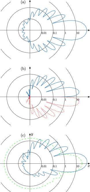
Figure 8: (Color online) Panel (a) shows a polar plot of the differential cross section, $d\sigma^{(+)}(\hat{\mathbf{k}}^{\prime},\hat{\mathbf{k}};E)/d\Omega_{\mathbf{k}^{\prime}}$, as a function of the in-plane scattering angle angle $\phi^{\prime}-\phi$ [Eqs. (64) and (66)], with incoming and outgoing momenta lying in the $xy$-plane, i.e. $\theta^{\prime}=\theta=\pi/2$ and $\hat{\mathbf{k}}=\mathbf{e}_{x}$ ($\phi=0$). The contours mark the magnitudes of the differential cross-sections in units of $\pi R^{2}$ on a log-scale. The quasiparticle energy is $E=1.01\Delta$, and the ion-quasiparticle potential is a hard sphere with $k_{f}R=11.17$. Similarly, panel (b) shows the asymmetry in the angular distribution of scattered quasiparticles given by $d\sigma^{(-)}(\hat{\mathbf{k}}^{\prime},\hat{\mathbf{k}};E)/d\Omega_{\mathbf{k}^{\prime}}$, which changes sign continuously across the lines $\Delta\phi=0,\pi$. The sign change is indicated by the dashed red curve. Panel (c) shows the sum of these two differentical cross-sections, highlighting the asymmetry in the angular distribution of scattering quasiparticles for $\mathbf{l}||\mathbf{z}$. The angular distribution for quasiparticle-ion scattering in the normal state is shown as the dashed green line.

In Fig. (8) we show results for the differential cross section defined in Eqs. (64) and (66) for in-plane scattering, i.e. both incident, $\mathbf{k}$, and scattered, $\mathbf{k}^{\prime}$, wavevectors in the $xy$-plane. In particular, for an incoming quasiparticle with $\hat{\mathbf{k}}=\mathbf{e}_{x}$ ($\theta=\pi/2,\phi=0$) the symmetric part of the angular distribution, $d\sigma^{(+)}/d\Omega_{\mathbf{k}^{\prime}}$, contributing to $\sigma^{(+)}_{ij}(E)$ is shown in panel (a), and the asymmetry in the angular distribution, $d\sigma^{(-)}/d\Omega_{\mathbf{k}^{\prime}}$, of the scattered excitations is shown in panel (b) as a function of the azimuthal scattering angle $\Delta\phi=\phi^{\prime}-\phi$. Note that $d\sigma^{(-)}/d\Omega_{\mathbf{k}^{\prime}}$ changes sign across the lines $\Delta\phi=0$ and $\Delta\phi=\pi$, and determines the anti-symmetric, transverse cross section, $\sigma^{(-)}_{ij}(E)$. The total differential cross-section is shown in Fig. (8c) in comparison with that for quasiparticle-ion scattering in the normal state. There is strong reduction in backscattering in the superfluid state compared to that in the normal state, as well as the sharp angular dependences associated with resonant scattering from the spectrum of chiral Fermions bound to the ion, evident in the angular momentum resolved density of states shown in Fig. (4). Resonant scattering of quasiparticles by the spectrum of chiral Fermions bound to the electron bubble is also evident in the energy-resolved transport cross-sections, $\sigma^{(-)}_{xy}(E)$ and $\sigma^{(+)}_{xx}(E)$, shown in Fig (9) normalized by the normal state transport cross section.

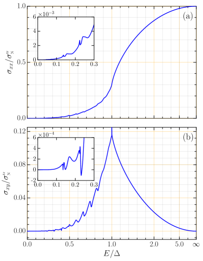
Figure 9: The longitudinal [panel (a)] and transverse [panel (b)] transport cross sections as a function of energy for $T=0.5T_{c}$. The peak-dip structure at energies below the maximum gap, $\Delta$, are resonances originating from scattering of quasiparticles by chiral Fermions bound to the surface of the electron bubble associated with distinct angular momentum channels [Eqs. (67)-(68)]. The quasiparticle-ion potential is a hard sphere with $k_{f}R=11.17$. The insets highlight the low-energy region.

One can clearly see the peak-dip structure at energies below the maximum gap $\Delta$. These structures are due to resonant scattering from chiral Fermions bound to the surface of the electron bubble. There is a resonance for each angular momentum channel $m$. The chiral Fermions form as a result of multiple potential and Andreev scattering of quasiparticles off the electron bubble and the chiral order parameter in which it is embedded. This multiple scattering and bound state formation is encoded in the $t$-matrix equations of Eqs. (25) - (28).

V.2 Forces on moving electron bubbles

The transport cross sections, $\sigma^{(+)}_{ij}(E)$ and $\sigma^{(-)}_{ij}(E)$ calculated for the hard sphere potential, are used to calculate the components of the Stokes tensor given in Eq. (65). In Fig. (10) we show our results for the temperature dependences of the longitudinal ($\eta_{xx}/\eta_{\text{N}}$) and transverse ($\eta_{xy}/\eta_{\text{N}}$) forces normalized to the normal state Stokes drag $\eta_{\text{N}}$. The longitudinal drag force drops rapidly below $T_{c}$ due to the (i) opening of the gap in the bulk excitation spectrum and (ii) resonant scattering reflected in terms of strong suppression of backscattering as shown in Fig. (8). The transverse force onsets at $T_{c}$, increases rapidly then decays at very low temperatures.

In the GL limit, $\Delta(T)/k_{\text{B}}T_{c}\sim(1-T/T_{c})^{\genfrac{}{}{}{1}{1}{2}}\ll 1$, the drag force decreases as $\eta_{xx}/\eta_{\text{N}}-1\propto-\Delta(T)$, while the transverse force scales as $\eta_{xy}/\eta_{\text{N}}\propto\Delta(T)^{2}\sim(1-T/T_{c})$, reflecting the onset of branch conversion scattering of Bogoliubov quasiparticles. The scaling near $T_{c}$ follows from the GL expansion of the cross-sections given in App. (D). The scaling of $\eta_{xy}\sim\Delta(T)^{2}$ agrees with that inferred from the estimate given in Eq. [1] of Ref. (Salmelin et al., 1989); however, these authors include an additional small factor, $k_{\text{B}}T_{c}/E_{f}\sim 10^{-3}$, typically associated with normal-state particle-hole asymmetry. In our theory, particle-hole asymmetry is generated by branch conversion scattering and particle-hole coherence that onsets at $T_{c}$, and is reflected in the asymmetric chiral spectrum for $d\sigma^{(-)}/d\Omega_{\mathbf{k}^{\prime}}(\mathbf{k}^{\prime},\mathbf{k};E)$. There is no factor, $k_{\text{B}}T_{c}/E_{f}$; however, there is a small factor originating from the small transverse momentum transfer that is a reflection of branch conversion scattering from the chiral order parameter. Our estimate of the longitudinal and transverse forces near $T_{c}$ for an electron bubble with velocity $v\,\mathbf{e}_{x}$ is as follows. For the moving ion encountering a flux $n\,v$, the typical momentum transfer imparted to the ion per quasiparticle (QP) collision is $\sim p_{f}$, and the momentum transport cross-section near $T_{c}$ is $\langle\sigma_{xx}\rangle\approx\sigma_{N}^{\text{tr}}\approx\pi R^{2}$, giving a drag force $|F_{x}|\approx n\,v\,p_{f}\,\sigma_{N}^{\text{tr}}$. Now for branch conversion scattering there is angular momentum transfer of $\hbar$ by the chiral order parameter per branch conversion scattering of a QP. Thus, the transverse momentum transfer is of order $\hbar/R$ per QP. Note that Andreev scattering is via the order parameter; there is no hard scattering with momentum transfer of order $p_{f}$. The fact that there is any momentum transfer is because of the angular momentum transfer via the chiral order parameter. In addition, branch conversion scattering onsets at $T_{c}$, thus the cross-section is reduced relative to that for the longitudinal force by the probability of branch conversion scattering of thermal Bogoliubov QPs near $T_{c}$, i.e. $\langle\sigma_{xy}\rangle\approx(\Delta(T)/k_{\text{B}}T_{c})^{2}\,\sigma_{N}^{\text{tr}}$, leading to $|F_{y}|\approx n\,v\,(\hbar/R)\langle\sigma_{xy}\rangle\approx n\,v\,(\hbar/R)\,\sigma_{N}^{\text{tr}}(\Delta(T)/k_{\text{B}}T_{c})^{2}$, and the ratio

$$\frac{|F_{y}|}{|F_{x}|}\simeq\frac{1}{k_{f}R}\,\left(\frac{\Delta(T)}{k_{\text{B}}T_{c}}\right)^{2}\,.$$ (70)

The factor $1/k_{f}R$ accounts for the relative size of the transverse and longitudinal transport cross-sections at $E\approx\Delta$ shown in Fig. (9), and also accounts for the order of magnitude reduction in the ratio $\eta_{xy}/\eta_{xx}$ shown in Fig. (10) at $T/T_{c}\approx 0.8$. Note that the transport cross sections, $\sigma_{xx}(E)$ and $\sigma_{xy}(E)$, were both defined by scaling out the dimensional factors of $p_{f}$ in the kinematics. Thus, $\sigma_{xy}(E)\simeq\genfrac{}{}{}{1}{\hbar}{p_{f}R}\sigma_{xx}(E)$ at $E\approx\Delta$. The spectral average, $\langle\sigma_{xy}(E)\rangle$ near $T_{c}$ generates the additional factor of $(\Delta/k_{\text{B}}T_{c})^{2}$. Although the transverse force is roughly an order of magnitude smaller than the drag force, it leads to a dramatic effect on the dynamics of the negative ion.

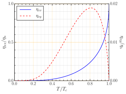
Figure 10: (Color online) Longitudinal and transverse Stokes parameters, $\eta_{xx}/\eta_{\text{N}}$ (solid blue line) and $\eta_{xy}/\eta_{\text{N}}$ (dashed red line), as a function of $T/T_{c}$. Calculations are based on the hard sphere quasiparticle-ion potential with $k_{f}R=11.17$.

The equation of motion for an electron bubble under the action of an in-plane electric field is

$$M\mbox{$\displaystyle\frac{d\mathbf{v}}{dt}$}=e\mathbf{E}-\eta_{\perp}\,\mathbf{v}-\eta_{xy}\,\mathbf{v}\times\hat{\mathbf{l}}\,,$$ (71)

where $M$ is the effective mass of the electron bubble. The first term on the right side of Eq. (71) is the Coulomb force on the ion, the second term is the drag force on the moving electron bubble, and the third term is the transverse force from the scattering of quasiparticles off Weyl Fermions bound to the ion. The drag force results in relaxation of the ion velocity on a timescale $\tau$ given by $1/\tau=\eta_{\perp}/M$, while the transverse force has the form of the Lorentz force, $\mathbf{F}_{\text{W}}=\genfrac{}{}{}{1}{e}{c}\,\mathbf{v}\times\mathbf{B}_{\text{W}}$, where the effective magnetic field arises from scattering of quasiparticles off the Weyl spectrum of the ion,

$$\mathbf{B}_{\text{W}} = -\frac{c}{e}\eta_{xy}\,\hat{\mathbf{l}}$$ (72)

$$\approx \frac{\Phi_{0}}{3\pi^{2}}\,k_{f}^{2}\,(k_{f}R)^{2}\,\left(\frac{\eta_{xy}}{\eta_{\text{N}}}\right)\,\hat{\mathbf{l}}\,,$$

where $\Phi_{0}=hc/2|e|$ is the flux quantum and we have approximated the normal state transport cross section by $\sigma_{\text{N}}^{\text{tr}}\approx\pi R^{2}$. Note that the temperature dependence of $B_{\text{W}}$ is shown in Fig. (10), and thus the order of magnitude of the Weyl field ranges from $B_{\text{W}}=10^{4}\,\mbox{T}$ at $T/T_{c}=0.8$ to $B_{\text{W}}=10^{3}\,\mbox{T}$ at $T/T_{c}=0.3$, orders of magnitude larger that any laboratory magnetic field.Ikegami et al. (2015)

The Weyl field and drag force generate damped cyclotron motion of the electron bubble with frequency, $\omega_{\text{c}}=eB_{\text{W}}/Mc$. The resulting steady-state velocity of the electron bubble in the combined electric ($\mathbf{E}=\mathcal{E}\mathbf{e}_{x}$) and Weyl ($\mathbf{B}_{\text{W}}=B_{\text{W}}\mathbf{e}_{z}$) fields is given by

$$v_{x}=\frac{\tau}{1+(\omega_{\text{c}}\tau)^{2}}\,e\mathcal{E}\,,\quad v_{y}=\frac{\tau(\omega_{\text{c}}\tau)}{1+(\omega_{\text{c}}\tau)^{2}}\,e\mathcal{E}\,.$$ (73)

The transverse component is the anomalous Hall current, and the ratio with the longitudinal current gives the Hall angle,

$$\tan\alpha=\frac{v_{y}}{v_{x}}=\omega_{\text{c}}\tau=\frac{eB_{\text{W}}}{Mc}\tau=\frac{\eta_{xy}}{\eta_{\perp}}\,.$$ (74)

Note that in spite of the enormous effective magnetic field, the Hall angle is relatively small because the relaxation time $\tau$ is so short compared to the cyclotron period, i.e. the drag force dominates the transverse force. At $T/T_{c}=0.8$, where the Weyl field is maximum, the Hall angle is of order $\tan\alpha=\eta_{xy}/\eta_{\perp}\approx 0.1$. The detailed temperature dependences of the Stokes parameters show that the maximum Hall angle is $\tan\alpha_{\text{max}}\approx 0.25$ at $T/T_{c}\approx 0.4$, as shown in Fig. (12), and discussed in more detail in comparison with the experimental measurements below.

V.3 Comparison between Theory and Experiment

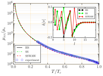
Figure 11: Experimental data for the longitudinal mobility normalized to the normal-state mobility is from Ref. [Ikegami et al., 2013] shown as blue circles. The theoretical result based on the hard sphere (HS) quasiparticle-ion potential is the black curve. Results based on the soft core (SS) potential are shown as the dashed green curve, and those for the four-parameter potential with intermediate attraction (SSWAW) are shown as the red dashed curve. Inset: Scattering phase shifts vs. angular momentum channel calculated for the three potentials. For the HS model: $k_{f}R=11.17$; SS model: $V_{0}=1.01\,E_{f}$ and $k_{f}R=12.48$; SSWAW model: $V_{0}=100\,E_{f}$ $V_{1}=10\,E_{f}$, $k_{f}R^{\prime}=10.99$ and $R/R^{\prime}=0.36$, all constrained by the experimental value of $\mu_{\text{N}}$.

The experimental results for the transport of electron bubbles in ³He are presented in terms of the components of the mobility tensor. The components of the mobility tensor are calculated from the Stokes parameters using Eqs. (54). In Fig. (11) we compare our theoretical result for the longitudinal mobility based on numerical calculations, using the machinery presented in the previous sections, with the experimental data reported in Refs. [Ikegami et al., 2013, 2015]. The hard sphere potential works remarkably well, reproducing the longitudinal mobility data for ³He-A over nearly two and a half decades for $0.25\lesssim T/T_{c}\leq 1$. It is worth emphasizing that the hard sphere potential is a single-parameter potential with the radius, $k_{f}R=11.17$, fixed by the normal-state mobility. There are no other adjustable parameters in the theory, thus the comparison between theory and experiment for $\mu_{xx}/\mu_{\text{N}}$ is essentially perfect down to $T\approx 250\,\mu\mbox{K}$.

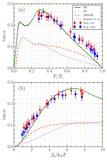
Figure 12: (Color online) Panel (a): Hall ratio for the motion of electron bubbles in ³He-A, $\tan\alpha\equiv v_{y}/v_{x}=\eta_{xy}/\eta_{xx}$, as a function of temperature for the hard sphere model for the quasiparticle-ion potential with $k_{f}R=11.17$ (black line). The experimental data was from the RIKEN group.Ikegami et al. (2013, 2015) Theoretical results for the repulsive soft core potential (dashed green line) and repulsive potential with short-range attraction (dashed red line) are shown for comparison. The dotted blue line corresponds to the calculation based on the formulas from Salmelin et al.Salmelin et al. (1989); Salmelin and Salomaa (1990) presented in Refs [Ikegami et al., 2013, 2015]. Panel (b): The same results presented as a function of $\Delta(T)/k_{B}T$.

We note that Ikegami et al.Ikegami et al. (2013) report a reasonably good comparison with their data, albeit with observable deviations at lower temperatures, using the incorrect formula for $\mu_{xx}/\mu_{\text{N}}$ from Ref. [Salmelin and Salomaa, 1990] with a hard sphere radius of $k_{f}R=16$. This much larger value disagrees with the radius obtained from measurements of the normal-state mobility. Moreover, as the authors of Ref. [Ikegami et al., 2013] found, the formula for the transverse mobility, $\mu_{xy}$, from Ref. [Salmelin and Salomaa, 1990] is in serious disagreement with experimental measurements of the transverse mobility as it under estimates the Hall angle by a factor of $\approx 2-4$ over a large temperature range, $0.25T_{c}\lesssim T\leq T_{c}$, based on the same value of $k_{f}R$. Again, the discrepancy originates from an incorrect formula for $\mu_{xy}$ reported in Ref. [Salmelin and Salomaa, 1990] (see App. (A)).

While the comparison of our theoretical prediction for $\mu_{xx}$ is excellent agreement with the RIKEN measurements, the strong test is the comparison of our calculations for the transverse force with the measurements of the anomalous Hall effect. In Fig. (12) we show our theoretical results [solid (black) curves] for the anomalous Hall ratio given by Eq. (74), with the calculated results for $\eta_{xy}$ and $\eta_{xx}$ (shown in Fig. (10)), plotted vs. $T/T_{c}$ in panel (a), and vs. $\Delta(T)/k_{\text{B}}T$ in panel (b). The (red) circular [(blue) square] symbols correspond to the experimental data reported in Refs. [Ikegami et al., 2013, 2015]. For comparison we include the results of the calculation by Ikegami et al. based on the formulae from Ref. [Salmelin and Salomaa, 1990] as the dotted (blue) lines.

It seems worth re-emphasizing that in all our calculations reported here the only parameter is hard sphere radius for the quasiparticle-ion potential which is fixed at the outset as $k_{f}R=11.17$ by the normal-state mobility. Thus, we view the overall agreement between theory and experiment as strong confirmation of the scattering theory, particularly the origin of the anomalous Hall effect resulting from resonant scattering of thermal quasiparticles by the spectrum of Weyl fermions bound to the electron bubble embedded in ³He-A.

The theoretical prediction shown in Fig. (12) shows structure in the Hall ratio - a dip-peak structure - below $T\approx 0.25\,T_{c}$. An important test of this theory would be measurements of the Hall mobility extended below $0.2\,\mbox{mK}$.

V.4 Beyond the hard sphere potential

Although the hard sphere model for the quasiparticle-ion potential provides very good agreement with the observed forces acting on the moving ion, it is a only rough approximation to expectations of the microscopic interaction between ³He quasiparticles and the electron bubble. To test the robustness of our theoretical predictions to the quasiparticle-ion potential we consider a more general central potential with short-range repulsion and intermediate-range attraction,

$$V(r)=\begin{cases}V_{0},&r\leq R\,,\\ -V_{1},&R<r\leq R^{\prime}\,,\\ 0,&r>R^{\prime}\,.\end{cases}$$ (75)

The normal-state scattering phase shifts for this piece-wise constant potential are expressed in terms of regular and modified spherical Bessel functions; the analytical formulas are given in Eqs. (105)-(107) of App. E. We discuss two cases both with $V_{0}>E_{f}$: (i) for $V_{1}=0$ the potential is a two-parameter, repulsive “soft-core” potential, and (ii) for $V_{1}>0$ and $R^{\prime}>R$ we include in addition to the short-range repulsion, an intermediate range attraction. The latter case allows for a shallow bound state, and corresponding scattering resonance, in one or more angular momentum channels, $l\leq l_{\text{max}}$.

Figures 11 and 12 show our calculations for the longitudinal mobility and Hall ratio for these potentials in comparison with the results for the hard sphere potential. The corresponding phase shifts are shown in the inset. For the “soft-core” model we chose a weakly repulsive potential, $V_{0}=1.01\,E_{f}\approx 0.5\mbox{meV}$, and adjusted the radius $R$ to fit the measured normal-state mobility, $\mu^{\text{exp}}_{\text{N}}=1.7\times 10^{-6}\,\mbox{m}^{2}/\mbox{V}/\mbox{s}$, as was done for the hard-sphere potential. The resulting phase shifts, shown in inset of Fig. (11), are similiar to those of calculated for hard-sphere scattering in that there are no additional strong scattering channels; the phase shift for the $l=5$ channel corresponds to strong scattering for both the hard sphere and the soft core potential. Furthermore, there is virtually no observable change in the theoretical predictions for the longitudinal and transverse forces on the moving ion described by the soft core potential, compared to the results for the hard sphere potential. This is representative of the general class of short-range repulsive potentials. So long as the range of the repulsive quasiparticle-ion potential is adjusted the fit the normal state mobility we obtain excellent agreement for the forces on the negative ion in the superfluid phase.Shevtsov and Sauls (2016)

The situation is different for the case with short-range repulsion and intermediate range attraction. Here we fixed $V_{0}=100\,E_{f}$ and $V_{1}=10\,E_{f}$, then adjusted $R$ and $R^{\prime}$ to obtain a best fit to the experimental value of the normal-state mobility, giving $k_{f}R^{\prime}=10.99$ and $R/R^{\prime}=0.36$. As can be seen from the inset of Fig. 11, the intermediate range attraction changes the set of scattering phase shifts, compared to the hard sphere potential, with the most dramatic change happening for $l=10$. This channel exhibits an additional scattering resonance [red triangles in the inset of Fig. (11)]. The scattering of quasiparticles in this channel is enhanced towards the unitary limit, $\delta_{l=10}\approx\pi/2$, which makes the partial scattering cross section for this channel maximal. As a consequence, the forces on the ion are modified. The longitudinal mobility shown in Fig. 11 (red dashed line) is slightly reduced compared to that for the hard sphere scattering potential. More dramatic is the reduction in the anomalous Hall ratio shown in Fig. (12), which deviates strongly from the experimental data (red dashed line). The main conclusion here is that for the negative ion the quaiparticle-ion scattering potential is repulsive and short range, and the experimental results are well described by hard sphere potential scattering.

A softer core potential with intermediate range attraction may be relevant to understanding the mobility of positive ions in ³He-A, given that the positive ion attracts ³He to form a “snowball” of ³He atoms with increased density relative to bulk ³He.Dobbs (2000) Indeed preliminary measurements of the longitudinal and transverse forces on a positive ion in ³He-A show different magnitudes and temperature dependences for the longitudinal mobility and anomalous Hall ratio compared to the negative ion.Ikegami et al. (2015) However, a detailed theoretical description of the structure and transport properties of the positive ion is outside the scope of this report.

VI Discussion

The comparison between theory and experiment for the Hall ratio shows a maximum deviation of $\approx 15\%$ at $T\approx 0.8T_{c}$, which is the temperature at which the transverse force, $\eta_{xy}$, is a maximum. This suggests that there may be an additional contribution to the transverse force on the moving ion. Within the theory of thermal quasiparticles scattering off the moving ion, the larger experimental value for $\eta_{xy}$ suggests an additional weak scattering mechanism contributing to the transport cross section, $\sigma_{xy}(E)$, at energies close to the gap edge, or perhaps deviations from the hard sphere potential. These possibilities for an additional contribution to the transverse force on the moving ion are addressed in a separate report.

It is also likely that in the low temperature limit, $T<0.25T_{c}$, new physics appears in the transport of electron bubbles in ³He-A. In particular, the theoretical prediction of the sub-gap spectrum shown in Fig. (11) leads to the sharp increase in the longitudinal mobility at low temperatures. Thus, at constant electric field we expect the linear theory for the Stokes force tensor to fail at sufficiently low temperatures as there is insufficient drag force from thermal quasiparticles to limit the ion velocity below the Landau critical velocity, $v_{c}=\Delta/p_{f}$. At high velocity the ion will dissipate energy by Cherenkov radiation of quasiparticles.Jensen and Sauls (1988) This process may onset at velocities well below $v_{c}$ given the low energy Weyl spectrum near the moving ion, and it is an open question as to whether and how the resulting quasiparticle radiation might contribute to transverse force.

Appendix A Critique of Salmelin and Salomaa’s Theory

The report by Salmelin and Salomaa (SS) on the mobility of electron bubbles in superfluid ³He-A was an attempt to extend the earlier work by Salomaa et al.Salomaa et al. (1980) on the same topic to calculate the transverse component of the mobility, $\mu_{xy}$. The latter was argued in Ref. [Salmelin et al., 1989] to exist based on the analogy of the Magnus effect for a spinning object moving through a fluid, in this case the electron bubble with bound circulating currents. While the physical argument in Ref. [Salmelin et al., 1989] for the transverse component of the mobility is sound, the formulation of the scattering theory by Salmelin et al.Salmelin et al. (1989); Salmelin and Salomaa (1990) cannot account for the transverse force on a moving electron bubble.

The primary error introduced by Salmelin et al.Salmelin et al. (1989); Salmelin and Salomaa (1990) in their formulation of the transport cross section for an electron bubble moving in superfluid ³He-A is the assumption of microscopic reversibility for scattering rates for the transition $\mathbf{k}\rightarrow\mathbf{k}^{\prime}$ and the inverse scattering event, $\mathbf{k}^{\prime}\rightarrow\mathbf{k}$, i.e. that $W(\mathbf{k}^{\prime},\mathbf{k})=W(\mathbf{k},\mathbf{k}^{\prime})$. However, ³He-A breaks mirror symmetry in any plane containing the chiral axis $\hat{\mathbf{l}}$, as well as time-reversal symmetry. Thus, the condition on the scattering rate for quasiparticles scattering off an ion in ³He-A connects the two scattering events for mirror reflected ground states, i.e. $W(\mathbf{k}^{\prime},\hat{\mathbf{k}};+\hat{\mathbf{l}})=W(\mathbf{k},\mathbf{k}^{\prime};-\hat{\mathbf{l}})$. Conversely, microscopic reversibility is violated for the broken symmetry ground state with fixed chirality $+\hat{\mathbf{l}}$.

By assuming microscopic reversibility the authors of Ref. [Salmelin and Salomaa, 1990] pre-supposed mirror symmetry in the scattering of quasiparticles off the electron bubble, and thus ensured that the Stokes tensor is symmetric and diagonal, i.e. that $\eta_{xy}=0$. This conclusion is clear from Eqs. [3],[5] and [6] of Salmelin et al.Salmelin and Salomaa (1990), and in the paragraph preceding Eqs. [4] of Ref. [Salmelin et al., 1989]. It is worth noting that the same assumption was made in the earlier work of Salomaa et al.Salomaa et al. (1980) for which there was no mention or calculation of a transverse force on the moving ion.

So, why do SS obtain a non-zero result for the transverse mobility? They introduce a second error in the evaluation of the kinematic factors, $(\hat{\mathbf{k}}^{\prime}-\hat{\mathbf{k}})_{i}(\hat{\mathbf{k}}^{\prime}-\mathbf{k})_{j}$ [$\Delta\mathbf{p}_{i}\Delta\mathbf{p}_{j}$ in the notation of SS]. Specifically, Eqs. [11] in SS are incorrect in their entirety. The argument in the paragraph preceding these formulae is the source of the error. SS generated Eqs. [11] by first assuming $\hat{\mathbf{k}}=\hat{\mathbf{e}}_{x}$ is fixed in the laboratory coordinate system such that the azimuthal angle $\phi_{\mathbf{k}}=0$. Then, the azimuthal angle for the final state momentum, $\mathbf{k}^{\prime}$, was replaced by $\phi_{\mathbf{k}^{\prime}}\rightarrow\phi_{\mathbf{k}^{\prime}}-\phi_{\mathbf{k}}$ to arrive at SS’s Eqs. [11]. This procedure is invalid, but has the effect of violating mirror symmetry in the kinematics. All kinematic factors, $\Delta\mathbf{k}_{i}\Delta\mathbf{k}_{j}$, are invariant under the mirror operation $\mathbf{k}\leftrightarrow\mathbf{k}^{\prime}$, in particular, $(\hat{\mathbf{k}}^{\prime}-\hat{\mathbf{k}})_{x}(\hat{\mathbf{k}}^{\prime}-\hat{\mathbf{k}})_{y}$ is invariant under $\mathbf{k}\leftrightarrow\mathbf{k}^{\prime}$, or equivalently under $\phi_{\mathbf{k}}\leftrightarrow\phi_{\mathbf{k}^{\prime}}$. Eq. [11] of SS for $\Delta\mathbf{k}_{x}\Delta\mathbf{k}_{y}$ violates mirror symmetry.

The result is a spurious transverse force from a mirror symmetric scattering rate. The violation of the mirror symmetry in the kinematic factors also predicts a spurious aniostropy of the drag force in the x-y plane, i.e. $\mu_{xx}\neq\mu_{yy}$, even in the isotropic normal Fermi liquid. The authors recoginized the violation of the axial symmetry of A phase excitation gap, so they enforced a single in-plane drag coefficient by replacing $\Delta\hat{\mathbf{k}}_{x}\Delta\hat{\mathbf{k}}_{x}\rightarrow\genfrac{}{}{}{1}{1}{2}\left(\Delta\hat{\mathbf{k}}_{x}\Delta\hat{\mathbf{k}}_{x}+\Delta\hat{\mathbf{k}}_{y}\Delta\hat{\mathbf{k}}_{y}\right)$ in the calculation of $\mu_{\perp}^{-1}$.

The erroneous set of Eqs. [11] in SS for the momentum transfer factors invalidates all the calculations of cross sections and components of the mobility tensor in Ref. [Salmelin and Salomaa, 1990] as well as Eqs. [4] in Ref. [Salmelin et al., 1989], and thus the source and magnitude of the transverse force on the moving electron bubble. In particular, the theory of SS, when evaluated with the correct formulae for the kinematic factors, $\Delta\hat{\mathbf{k}}_{i}\Delta\hat{\mathbf{k}}_{j}$ yields only uniaxal Stokes drag forces and zero transverse force on the moving ion, as was originally obtained in Ref. [Salomaa et al., 1980].

Our formulation of the force on the moving ion incorporates broken time reversal and mirror symmetries by the ³He-A ground state correctly. We are able to identify scattering events that contribute to the Stokes drag and the transverse force as, $W^{(+)}(\mathbf{k}^{\prime},\mathbf{k})=+W^{(+)}(\mathbf{k},\mathbf{k}^{\prime})$ and $W^{(-)}(\mathbf{k}^{\prime},\mathbf{k})=-W^{(-)}(\mathbf{k},\mathbf{k}^{\prime})$, respectively. Mirror symmetric scattering generates the drag forces, while the anti-symmetric component to the rate is responsible for the transverse force and the anomalous Hall effect, as we discuss in Sec. (IV.3).

Appendix B Kernel for the LDOS near the electron bubble

The kernel, $K_{l^{\prime}l}^{m}(u^{\prime},u,\varepsilon)$ (Eq. (37), defining the LDOS and the current density is obtained from the trace of the Nambu Green’s function $\widehat{\mathcal{G}}^{\text{R}}_{\text{S}}(\mathbf{r},\mathbf{r};E)$ in Eqs. (31 - 33). Only the $t$-matrix term in Eq. (33) contributes to the kernel, in which case we are led to evaluate the integral

$$\mathrm{I}=\int\frac{d^{3}k^{\prime}}{(2\pi)^{3}}\int\frac{d^{3}k}{(2\pi)^{3}}e^{i(\mathbf{k}^{\prime}-\mathbf{k})\cdot\mathbf{r}}\widehat{G}^{\text{R}}_{\text{S}}(\mathbf{k}^{\prime},E)\widehat{T}^{\text{R}}_{\text{S}}(\mathbf{k}^{\prime},\mathbf{k};E)\widehat{G}^{\text{R}}_{\text{S}}(\mathbf{k},E)\,.$$ (76)

We use Eq. (32) and utilize the expansion of the plane wave, $e^{i\mathbf{k}\cdot\mathbf{r}}=4\pi\sum_{l=0}^{\infty}\sum_{m=-l}^{l}i^{l}j_{l}(kr)Y_{l}^{m}(\hat{\mathbf{k}})Y_{l}^{m}(\hat{\mathbf{r}})^{\ast}$, in spherical harmonics and the regular spherical Bessel functions. In the quasiclassical limit, $E_{f}\ll\Delta$ (see Note Note, 5), we evaluate the $t$-matrix in the elastic limit for momenta on Fermi surface and obtain

$$\mathrm{I} =(4\pi N_{f})^{2}\sum_{l,l^{\prime}=0}^{\infty}\sum_{m^{\prime}=-l^{\prime}}^{l^{\prime}}\sum_{m=-l}^{l}i^{l^{\prime}-l}Y_{l^{\prime}}^{m^{\prime}}(\hat{\mathbf{r}})^{\ast}Y_{l}^{m}(\hat{\mathbf{r}})\int\frac{d\Omega_{\mathbf{k}^{\prime}}}{4\pi}\int\frac{d\Omega_{\mathbf{k}}}{4\pi}Y_{l^{\prime}}^{m^{\prime}}(\hat{\mathbf{k}}^{\prime})Y_{l}^{m}(\hat{\mathbf{k}})^{\ast}$$

$$\times\left[\int_{-\infty}^{\infty}d\xi^{\prime}j_{l^{\prime}}(k^{\prime}r)\widehat{G}^{\text{R}}_{\text{S}}(\mathbf{k}^{\prime},E)\right]\widehat{T}^{\text{R}}_{\text{S}}(\hat{\mathbf{k}}^{\prime},\hat{\mathbf{k}};E)\left[\int_{-\infty}^{\infty}d\xi j_{l}(kr)\widehat{G}^{\text{R}}_{\text{S}}(\mathbf{k},E)\right]\,.$$ (77)

The remaining integral

$$\mathrm{J}=\int_{-\infty}^{\infty}d\xi j_{l}(kr)\widehat{G}^{\text{R}}_{\text{S}}(\mathbf{k},E),$$ (78)

is evaluated most conveniently using spherical Hankel functions of the first and second kind,

$$h_{l}^{(1,2)}(x)=j_{l}(x)\pm in_{l}(x)\,,\quad\mbox{where}\quad h_{l}^{(1,2)}(x)\propto e^{\pm ix}\,,$$ (79)

in which case we obtain,

$$\mathrm{J}=\frac{1}{2}\left[h_{l}^{(1)}(k_{f}r)\,\mathrm{J}^{+}+h_{l}^{(2)}(k_{f}r)\,\mathrm{J}^{-}\right]\,,$$ (80)

$$\mathrm{J}^{\pm}\equiv\int d\xi\,e^{\pm i\frac{\xi}{\hbar v_{f}}r}\,\widehat{G}^{\text{R}}_{\text{S}}(\mathbf{k},E)\,,$$ (81)

where we used $k=k_{f}+\xi/\hbar v_{f}$. The integrals $\mathrm{J}^{\pm}$ are evaluated using Eq. (16),

$$\mathrm{J}^{\pm}=-i\pi e^{-\sqrt{|\Delta(\hat{\mathbf{k}})|^{2}-\varepsilon^{2}}\frac{r}{\hbar v_{f}}}\left[\frac{-i}{\sqrt{|\Delta(\hat{\mathbf{k}})|^{2}-\varepsilon^{2}}}\begin{pmatrix}\varepsilon\mathbb{1}&-\hat{\Delta}(\hat{\mathbf{k}})\\ -\hat{\Delta}^{\dagger}(\hat{\mathbf{k}})&\varepsilon\mathbb{1}\end{pmatrix}\pm\begin{pmatrix}\mathbb{1}&0\\ 0&-\mathbb{1}\\ \end{pmatrix}\right]\,.$$ (82)

Expressing the spherical harmonics as $Y_{l}^{m}(\hat{\mathbf{k}})\equiv Y_{l}^{m}(\theta,\phi)=\Theta_{l}^{m}(\cos\theta)\,e^{im\phi}$, we then integrate over the azimuthal angles in Eq. (77). Finally, Eq. (36) is obtained by evaluating the trace over the Nambu matrices in Eq. (77),

$$\sum_{m=-\infty}^{\infty}\delta N_{m}(\mathbf{r},E)=-\frac{1}{2\pi}\mathrm{Im}\left[\mathrm{Tr}(\mathrm{I})\right].$$ (83)

Appendix C Formulae for the electron bubble current density

The current density circulating an electron bubble in cartesian components is $\mathbf{j}(r,\vartheta,\varphi)=\sum_{i=x,y,z}\,j_{i}(\mathbf{r})\,\hat{\mathbf{e}}_{i}$. The current along the chiral axis,

$$j_{z}(\mathbf{r}) = -4\pi^{3}v_{f}N_{f}k_{B}T\,\mathrm{Re}\Biggl{\{}\sum_{n=0}^{\infty}\sum_{m=-\infty}^{\infty}\sum_{l,l^{\prime}=|m|}^{\infty}\Theta_{l^{\prime}}^{m}(\cos\vartheta)\Theta_{l}^{m}(\cos\vartheta)\int_{-1}^{1}du^{\prime}\int_{-1}^{1}du(u^{\prime}+u)$$ (84)

$$\times \Theta_{l^{\prime}}^{m}(u^{\prime})e^{-\sqrt{\Delta^{2}(1-u^{\prime 2})+\varepsilon_{n}^{2}}\frac{r}{\hbar v_{f}}}\Theta_{l}^{m}(u)e^{-\sqrt{\Delta^{2}(1-u^{2})+\varepsilon_{n}^{2}}\frac{r}{\hbar v_{f}}}K_{l^{\prime}l}^{m}(u^{\prime},u,i\epsilon_{n})\Biggr{\}}\,,$$

vanishes by symmetry; in particular, the spectrum of Weyl fermions is symmetric under $z\rightarrow-z$. The in-plane components are expressed in terms for the four terms related to the components of the $t$-matrix,

$$j_{x}(\mathbf{r})=-4\pi^{3}v_{f}N_{f}k_{B}T\,\mathrm{Re}\Biggl{\{}\sum_{n=0}^{\infty}\sum_{m=-\infty}^{\infty}\frac{1}{2}\Bigl{[}j_{1}^{m}(\mathbf{r},\epsilon_{n})+j_{2}^{m}(\mathbf{r},\epsilon_{n})+j_{3}^{m}(\mathbf{r},\epsilon_{n})+j_{4}^{m}(\mathbf{r},\epsilon_{n})\Bigr{]}\Biggr{\}}\,,$$ (85)

$$j_{y}(\mathbf{r})=-4\pi^{3}v_{f}N_{f}k_{B}T\,\mathrm{Re}\Biggl{\{}\sum_{n=0}^{\infty}\sum_{m=-\infty}^{\infty}\frac{1}{2i}\Bigl{[}j_{1}^{m}(\mathbf{r},\epsilon_{n})-j_{2}^{m}(\mathbf{r},\epsilon_{n})+j_{3}^{m}(\mathbf{r},\epsilon_{n})-j_{4}^{m}(\mathbf{r},\epsilon_{n})\Bigr{]}\Biggr{\}},$$ (86)

where

$$j_{1}^{m}(\mathbf{r},\epsilon_{n}) =e^{i\varphi}\sum_{l^{\prime}=|m-1|}^{\infty}\sum_{l=|m|}^{\infty}\Theta_{l^{\prime}}^{m-1}(\cos\vartheta)\Theta_{l}^{m}(\cos\vartheta)\int_{-1}^{1}du^{\prime}\int_{-1}^{1}du\sqrt{1-u^{\prime 2}}$$

$$\times\Theta_{l^{\prime}}^{m-1}(u^{\prime})e^{-\sqrt{\Delta^{2}(1-u^{\prime 2})+\varepsilon_{n}^{2}}\frac{r}{\hbar v_{f}}}\Theta_{l}^{m}(u)e^{-\sqrt{\Delta^{2}(1-u^{2})+\varepsilon_{n}^{2}}\frac{r}{\hbar v_{f}}}K_{l^{\prime}l}^{m}(u^{\prime},u,i\epsilon_{n})\,,$$ (87)

$$j_{2}^{m}(\mathbf{r},\epsilon_{n}) =e^{-i\varphi}\sum_{l^{\prime}=|m+1|}^{\infty}\sum_{l=|m|}^{\infty}\Theta_{l^{\prime}}^{m+1}(\cos\vartheta)\Theta_{l}^{m}(\cos\vartheta)\int_{-1}^{1}du^{\prime}\int_{-1}^{1}du\sqrt{1-u^{\prime 2}}$$

$$\times\Theta_{l^{\prime}}^{m+1}(u^{\prime})e^{-\sqrt{\Delta^{2}(1-u^{\prime 2})+\varepsilon_{n}^{2}}\frac{r}{\hbar v_{f}}}\Theta_{l}^{m}(u)e^{-\sqrt{\Delta^{2}(1-u^{2})+\varepsilon_{n}^{2}}\frac{r}{\hbar v_{f}}}K_{l^{\prime}l}^{m}(u^{\prime},u,i\epsilon_{n})\,,$$ (88)

$$j_{3}^{m}(\mathbf{r},\epsilon_{n}) =e^{i\varphi}\sum_{l^{\prime}=|m|}^{\infty}\sum_{l=|m+1|}^{\infty}\Theta_{l^{\prime}}^{m}(\cos\vartheta)\Theta_{l}^{m+1}(\cos\vartheta)\int_{-1}^{1}du^{\prime}\int_{-1}^{1}du\sqrt{1-u^{2}}$$

$$\times\Theta_{l^{\prime}}^{m}(u^{\prime})e^{-\sqrt{\Delta^{2}(1-u^{\prime 2})+\varepsilon_{n}^{2}}\frac{r}{\hbar v_{f}}}\Theta_{l}^{m+1}(u)e^{-\sqrt{\Delta^{2}(1-u^{2})+\varepsilon_{n}^{2}}\frac{r}{\hbar v_{f}}}K_{l^{\prime}l}^{m}(u^{\prime},u,i\epsilon_{n})\,,$$ (89)

$$j_{4}^{m}(\mathbf{r},\epsilon_{n}) =e^{-i\varphi}\sum_{l^{\prime}=|m|}^{\infty}\sum_{l=|m-1|}^{\infty}\Theta_{l^{\prime}}^{m}(\cos\vartheta)\Theta_{l}^{m-1}(\cos\vartheta)\int_{-1}^{1}du^{\prime}\int_{-1}^{1}du\sqrt{1-u^{2}}$$

$$\times\Theta_{l^{\prime}}^{m}(u^{\prime})e^{-\sqrt{\Delta^{2}(1-u^{\prime 2})+\varepsilon_{n}^{2}}\frac{r}{\hbar v_{f}}}\Theta_{l}^{m-1}(u)e^{-\sqrt{\Delta^{2}(1-u^{2})+\varepsilon_{n}^{2}}\frac{r}{\hbar v_{f}}}K_{l^{\prime}l}^{m}(u^{\prime},u,i\epsilon_{n}).$$ (90)

Using the following symmetry properties of the kernel, $K_{l^{\prime}l}^{m}(u^{\prime},u,i\epsilon_{n})\equiv i^{l^{\prime}-l}\kappa_{l^{\prime}l}^{m}(u^{\prime},u,i\epsilon_{n})$,

$$\kappa_{l^{\prime}l}^{-m}(u^{\prime},u,i\epsilon_{n})=-\left[\kappa_{l^{\prime}l}^{m}(u^{\prime},u,i\epsilon_{n})\right]^{\ast}\,,$$ (91)

$$\kappa_{ll^{\prime}}^{m}(u,u^{\prime},i\epsilon_{n})=\kappa_{l^{\prime}l}^{m}(u^{\prime},u,i\epsilon_{n})\,,$$ (92)

one finds that the current density is purely azimuthal, $\mathbf{j}(r,\vartheta,\varphi)=j_{\varphi}(r,\vartheta)\,\mathbf{e}_{\varphi}\,\,,\mbox{with}\,\,\mathbf{e}_{\varphi}=-\sin\varphi\mathbf{e}_{x}+\cos\varphi\mathbf{e}_{y}$,

$$j_{\varphi}(r,\vartheta) =-8\pi^{3}v_{f}N_{f}k_{B}T\,\sum_{n=0}^{\infty}\sum_{m=-\infty}^{\infty}\sum_{l^{\prime}=|m-1|}^{\infty}\sum_{l=|m|}^{\infty}\Theta_{l^{\prime}}^{m-1}(\cos\vartheta)\Theta_{l}^{m}(\cos\vartheta)\int_{-1}^{1}du^{\prime}\int_{-1}^{1}du\sqrt{1-u^{\prime 2}}$$

$$\times\Theta_{l^{\prime}}^{m-1}(u^{\prime})e^{-\sqrt{\Delta^{2}(1-u^{\prime 2})+\epsilon_{n}^{2}}\frac{r}{\hbar v_{f}}}\Theta_{l}^{m}(u)e^{-\sqrt{\Delta^{2}(1-u^{2})+\epsilon_{n}^{2}}\frac{r}{\hbar v_{f}}}\mathrm{Re}\left[\kappa_{l^{\prime}l}^{m}(u^{\prime},u,i\epsilon_{n})\right]\mathrm{Im}\left[i^{l^{\prime}-l}\right]\,.$$ (93)

Appendix D Formulae for the scattering rate and transport cross section

We summarize our results for the transport cross sections in terms of the solutions to the coupled Eqs. (25)-(28) for the $t$-matrix. Given the solutions for the branch components, $t_{a}^{m}$, we substitute Eqs. (25)-(28) into Eq. (IV.1), to obtain

$$W(\hat{\mathbf{k}}^{\prime},\hat{\mathbf{k}})=\frac{1}{\pi^{2}N_{F}^{2}}\sum_{m=-\infty}^{\infty}\sum_{m^{\prime}=-\infty}^{\infty}e^{-i(m^{\prime}-m)(\phi^{\prime}-\phi)}\Biggl{\{}$$

$$\left[t_{1}^{m}(u^{\prime},u)^{\ast}+(-1)^{m+1}\frac{\Delta\sqrt{1-u^{2}}}{E}e^{-i(\phi^{\prime}-\phi)}t_{2}^{m}(u^{\prime},-u)^{\ast}\right]\times\left[t_{1}^{m^{\prime}}(u^{\prime},u)+(-1)^{m^{\prime}}\frac{\Delta\sqrt{1-u^{\prime 2}}}{E}t_{3}^{m^{\prime}}(-u^{\prime},u)\right]$$

$$+ \left[(-1)^{m+1}t_{2}^{m}(u^{\prime},-u)^{\ast}+\frac{\Delta\sqrt{1-u^{2}}}{E}e^{i(\phi^{\prime}-\phi)}t_{1}^{m}(u^{\prime},u)^{\ast}\right]\times\left[(-1)^{m^{\prime}+1}t_{2}^{m^{\prime}}(u^{\prime},-u)+\frac{\Delta\sqrt{1-u^{\prime 2}}}{E}t_{4}^{m^{\prime}}(-u^{\prime},-u)\right]$$

$$+ \left[(-1)^{m}t_{3}^{m}(-u^{\prime},u)^{\ast}+\frac{\Delta\sqrt{1-u^{2}}}{E}e^{-i(\phi^{\prime}-\phi)}t_{4}^{m}(-u^{\prime},-u)^{\ast}\right]\times\left[(-1)^{m^{\prime}}t_{3}^{m^{\prime}}(-u^{\prime},u)+\frac{\Delta\sqrt{1-u^{\prime 2}}}{E}t_{1}^{m^{\prime}}(u^{\prime},u)\right]$$

$$+ \left[t_{4}^{m}(-u^{\prime},-u)^{\ast}+(-1)^{m}\frac{\Delta\sqrt{1-u^{2}}}{E}e^{i(\phi^{\prime}-\phi)}t_{3}^{m}(-u^{\prime},u)^{\ast}\right]\times\left[t_{4}^{m^{\prime}}(-u^{\prime},-u)+(-1)^{m^{\prime}+1}\frac{\Delta\sqrt{1-u^{\prime 2}}}{E}t_{2}^{m^{\prime}}(u^{\prime},-u)\right]\Biggr{\}}.$$ (94)

A key feature of the scattering rate is the dependence on the azimuthal angles for the incident and outgoing momenta only in the combination $(\phi^{\prime}-\phi)$. This greatly simplifies the calculation of the transport cross sections [see Eqs. (67)-(68)], since any other combination of $\phi^{\prime}$ and $\phi$ gives zero contribution after integration over incident and final state momenta. This allows us to show the following,

$$\sigma^{(+)}_{xy}(E) = \sigma^{(+)}_{yx}(E)=0\,,$$ (95)

$$\sigma^{(\pm)}_{xz}(E) = \sigma^{(\pm)}_{zx}(E)=\sigma^{(\pm)}_{yz}(E)=\sigma^{(\pm)}_{zy}(E)=0\,,$$ (96)

$$\sigma^{(+)}_{xx}(E) = \sigma^{(+)}_{yy}(E)\,,$$ (97)

$$\sigma^{(-)}_{xy}(E) = -\sigma^{(-)}_{yx}(E)\,.$$ (98)

To carry out calculations we project out scattering rates with difference orbital angular momenta, $\Delta m=0,\pm 1$,

$$\frac{2\pi}{k_{F}^{2}}W_{0}(u^{\prime},u) = \left(\frac{m^{\ast}}{2\pi\hbar^{2}}\right)^{2}\int\limits_{0}^{2\pi}d\phi\int\limits_{0}^{2\pi}\frac{d\phi^{\prime}}{2\pi}W(\hat{\mathbf{k}}^{\prime},\hat{\mathbf{k}})\,,$$ (99)

$$\frac{2\pi}{k_{F}^{2}}W_{\pm}(u^{\prime},u) = \left(\frac{m^{\ast}}{2\pi\hbar^{2}}\right)^{2}\int\limits_{0}^{2\pi}d\phi\int\limits_{0}^{2\pi}\frac{d\phi^{\prime}}{2\pi}\,e^{\pm i(\phi^{\prime}-\phi)}\,W(\hat{\mathbf{k}}^{\prime},\hat{\mathbf{k}})$$ (100)

These rates are expressed in terms of solutions to the $t$-matrix amplitudes,

$$W_{0}(u^{\prime},u)=\sum_{m=-\infty}^{\infty}\Biggl{\{}$$

$$\left[t_{1}^{m}(u^{\prime},u)^{\ast}+(-1)^{m}\frac{\Delta\sqrt{1-u^{2}}}{E}t_{2}^{m+1}(u^{\prime},-u)^{\ast}\right]\times\left[t_{1}^{m}(u^{\prime},u)+(-1)^{m}\frac{\Delta\sqrt{1-u^{\prime 2}}}{E}t_{3}^{m}(-u^{\prime},u)\right]$$

$$+ \left[(-1)^{m+1}t_{2}^{m}(u^{\prime},-u)^{\ast}+\frac{\Delta\sqrt{1-u^{2}}}{E}t_{1}^{m-1}(u^{\prime},u)^{\ast}\right]\times\left[(-1)^{m+1}t_{2}^{m}(u^{\prime},-u)+\frac{\Delta\sqrt{1-u^{\prime 2}}}{E}t_{4}^{m}(-u^{\prime},-u)\right]$$

$$+ \left[(-1)^{m}t_{3}^{m}(-u^{\prime},u)^{\ast}+\frac{\Delta\sqrt{1-u^{2}}}{E}t_{4}^{m+1}(-u^{\prime},-u)^{\ast}\right]\times\left[(-1)^{m}t_{3}^{m}(-u^{\prime},u)+\frac{\Delta\sqrt{1-u^{\prime 2}}}{E}t_{1}^{m}(u^{\prime},u)\right]$$

$$+ \left[t_{4}^{m}(-u^{\prime},-u)^{\ast}+(-1)^{m-1}\frac{\Delta\sqrt{1-u^{2}}}{E}t_{3}^{m-1}(-u^{\prime},u)^{\ast}\right]\times\left[t_{4}^{m}(-u^{\prime},-u)+(-1)^{m+1}\frac{\Delta\sqrt{1-u^{\prime 2}}}{E}t_{2}^{m}(u^{\prime},-u)\right]\Biggr{\}}\,,$$ (101)

$$W_{\pm}(u^{\prime},u)=\sum_{m=-\infty}^{\infty}\Biggl{\{}$$

$$\left[t_{1}^{m\mp 1}(u^{\prime},u)^{\ast}+(-1)^{m\mp 1}\frac{\Delta\sqrt{1-u^{2}}}{E}t_{2}^{m\mp 1+1}(u^{\prime},-u)^{\ast}\right]\times\left[t_{1}^{m}(u^{\prime},u)+(-1)^{m}\frac{\Delta\sqrt{1-u^{\prime 2}}}{E}t_{3}^{m}(-u^{\prime},u)\right]$$

$$+ \left[(-1)^{m\mp 1+1}t_{2}^{m\mp 1}(u^{\prime},-u)^{\ast}+\frac{\Delta\sqrt{1-u^{2}}}{E}t_{1}^{m\mp 1-1}(u^{\prime},u)^{\ast}\right]\times\left[(-1)^{m+1}t_{2}^{m}(u^{\prime},-u)+\frac{\Delta\sqrt{1-u^{\prime 2}}}{E}t_{4}^{m}(-u^{\prime},-u)\right]$$

$$+ \left[(-1)^{m\mp 1}t_{3}^{m\mp 1}(-u^{\prime},u)^{\ast}+\frac{\Delta\sqrt{1-u^{2}}}{E}t_{4}^{m\mp 1+1}(-u^{\prime},-u)^{\ast}\right]\times\left[(-1)^{m}t_{3}^{m}(-u^{\prime},u)+\frac{\Delta\sqrt{1-u^{\prime 2}}}{E}t_{1}^{m}(u^{\prime},u)\right]$$

$$+ \left[t_{4}^{m\mp 1}(-u^{\prime},-u)^{\ast}+(-1)^{m\mp 1-1}\frac{\Delta\sqrt{1-u^{2}}}{E}t_{3}^{m\mp 1-1}(-u^{\prime},u)^{\ast}\right]\times\left[t_{4}^{m}(-u^{\prime},-u)+(-1)^{m+1}\frac{\Delta\sqrt{1-u^{\prime 2}}}{E}t_{2}^{m}(u^{\prime},-u)\right]\Biggr{\}}.$$ (102)

Formulae for the in-plane transport cross sections are given in terms of integrations over $W_{0,\pm}(u^{\prime},u;E)$,

$$\sigma^{(+)}_{xx}(E) = \frac{3\pi}{4k_{F}^{2}}\int_{E\geq|\Delta(\hat{\mathbf{k}})|}du\int_{E\geq|\Delta(\hat{\mathbf{k}}^{\prime})|}du^{\prime}\frac{E^{2}}{\sqrt{E^{2}-|\Delta(\hat{\mathbf{k}})|^{2}}\sqrt{E^{2}-|\Delta(\hat{\mathbf{k}}^{\prime})|^{2}}}\Biggl{\{}$$ (103)

$$\times \left(1-\frac{u^{2}+u^{\prime 2}}{2}\right)\,W_{0}(u^{\prime},u)-\frac{1}{2}\sqrt{1-u^{2}}\sqrt{1-u^{\prime 2}}\left[W_{+}(u^{\prime},u)+W_{-}(u^{\prime},u)\right]\Biggr{\}}\,,$$

$$\sigma^{(-)}_{xy}(E) = \frac{3\pi}{4k_{F}^{2}}\int_{E\geq|\Delta(\hat{\mathbf{k}})|}du\int_{E\geq|\Delta(\hat{\mathbf{k}}^{\prime})|}du^{\prime}\frac{E^{2}}{\sqrt{E^{2}-|\Delta(\hat{\mathbf{k}})|^{2}}\sqrt{E^{2}-|\Delta(\hat{\mathbf{k}}^{\prime})|^{2}}}\Biggl{\{}$$ (104)

$$\times \frac{1-2f}{4i}\sqrt{1-u^{2}}\sqrt{1-u^{\prime 2}}\left[W_{+}(u^{\prime},u)-W_{-}(u^{\prime},u)+W_{+}(u,u^{\prime})-W_{-}(u,u^{\prime})\right]\Biggr{\}}\,.$$

The other elements of the tensor cross sections are obtained by the symmetry relations, Eqs. (95) - (98).

Appendix E Scattering phase shifts for quasiparticle-ion potentials

For the potential defined by Eq. (75) the scattering phase shifts for normal-state quasiparticles are calculated from the following expressions,

$$\tan\delta_{l}=\frac{(l-\gamma_{l})j_{l}(k_{f}R^{\prime})-k_{f}R^{\prime}j_{l+1}(k_{f}R^{\prime})}{(l-\gamma_{l})n_{l}(k_{f}R^{\prime})-k_{f}R^{\prime}n_{l+1}(k_{f}R^{\prime})}\,,\;\;\gamma_{l}=x^{\prime}\frac{a_{l}}{b_{l}},$$ (105)

$$a_{l} =l\left[n_{l+1}(x)j_{l}(x^{\prime})-n_{l}(x^{\prime})j_{l+1}(x)\right]+x^{\prime}\left[n_{l+1}(x^{\prime})j_{l+1}(x)-n_{l+1}(x)j_{l+1}(x^{\prime})\right]$$

$$+\frac{lp_{l}}{x^{\prime}}\left[n_{l}(x)j_{l}(x^{\prime})-n_{l}(x^{\prime})j_{l}(x)\right]+p_{l}\left[n_{l+1}(x^{\prime})j_{l}(x)-n_{l}(x)j_{l+1}(x^{\prime})\right],$$ (106)

$$b_{l} =x^{\prime}\left[n_{l+1}(x)j_{l}(x^{\prime})-n_{l}(x^{\prime})j_{l+1}(x)\right]+p_{l}\left[n_{l}(x)j_{l}(x^{\prime})-n_{l}(x^{\prime})j_{l}(x)\right],$$ (107)

and $p_{l}=z^{\prime}i_{l+1}(z)/i_{l}(z)$ with $x=\beta_{1}k_{f}R$, $x^{\prime}=\beta_{1}k_{f}R^{\prime}$, $z=\beta_{0}k_{f}R$, $z^{\prime}=\beta_{0}k_{f}R^{\prime}$, $\beta_{0}=\sqrt{\genfrac{}{}{}{1}{V_{0}-E_{f}}{E_{f}}}$ and $\beta_{1}=\sqrt{\genfrac{}{}{}{1}{E_{f}+V_{1}}{E_{f}}}$, where $i_{l}(x)$ is the modified spherical Bessel function of the first kind.

References

- Anderson and Morel (1960) P. W. Anderson and P. Morel. Generalized Bardeen-Cooper-Schrieffer States and Aligned Orbital Angular Momentum in the Proposed Low-Temperature Phase of Liquid 3He. Phys. Rev. Lett., 5:136–138, 1960.
- Volovik (1975) G. Volovik. Angular momentum and orbital waves in the anisotropic A phase of superfluid 3He. Sov. Phys. JETP Lett., 22(4):108, 1975. [ZhETF Pis. Red., 22, 234 (1975)].
- Cross (1977) M. C. Cross. Orbital dynamics of the Anderson-Brinkman-Morel phase of superfluid 3He. J. Low Temp. Phys., 26:165–191, 1977.
- Ishikawa (1977) M. Ishikawa. Orbital angular momentum of anisotropic superfluid. Prog. Theor. Phys., 57:1836–1847, 1977.
- Leggett and Takagi (1978) A. J. Leggett and S. Takagi. Orientational dynamics of superfluid 3He: A “two-fluid” model. II. Orbital dynamics. Ann. Phys., 110(2):353–406, 1978.
- McClure and Takagi (1979) M. G. McClure and S. Takagi. Angular momentum of anisotropic superfluids. Phys. Rev. Lett., 43:596–598, 1979.
- Rainer and Vuorio (1977) D. Rainer and M. Vuorio. Small Objects in Superfluid 3He. J. Phys. C, 10(16):3093–3106, 1977.
- Ikegami et al. (2013) H. Ikegami, Y. Tsutsumi, and K. Kono. Chiral Symmetry in Superfluid 3He-A. Science, 341(6141):59–62, 2013.
- Ikegami et al. (2015) H. Ikegami, Y. Tsutsumi, and K. Kono. Observation of Intrinsic Magnus Force and Direct Detection of Chirality in Superfluid 3He-A. J. Phys. Soc. Jpn., 84(4):044602, 2015.
- Sauls (2011) J. A. Sauls. Surface states, Edge Currents, and the Angular Momentum of Chiral -wave Superfluids. Phys. Rev. B, 84:214509, 2011.
- Volovik and Mineev (1981) G. E. Volovik and V. P. Mineev. Orbital Angular Momentum and Orbital Dynamics: 3He-A and the Bose Liquid. Sov. Phys. JETP, 81:989, 1981.
- Hatsugai (1993) Y. Hatsugai. Chern number and edge states in the integer quantum Hall effect. Phys. Rev. Lett., 71:3697–3700, 1993.
- Volovik (2016) G. E. Volovik. Topological Superfluids. arXiv, 1602.02595, 2016.
- Mizushima et al. (2016) T. Mizushima, Y. Tsutsumi, T. Kawakami, M. Sato, M. Ichioka, and K. Machida. Symmetry Protected Topological Superfluids and Superconductors. J. Phys. Soc. Jpn., 85:022001, 2016.
- Read and Green (2000) N. Read and D. Green. Paired states of Fermions in two dimensions with breaking of parity and time-reversal symmetries and the fractional quantum Hall effect. Phys. Rev. B, 61(15):10267–10297, 2000.
- Volovik (1988) G. E. Volovik. An analog of the quantum Hall effect in a superfluid 3He film. Sov. Phys. JETP, 67:1804, 1988.
- Volovik (1992a) G. E. Volovik. Quantum Hall state and chiral edge state in thin 3He-A film. JETP Lett., 55(6):368–373, 1992a. [Pis’ma ZhETF, 55, 363 (1992)].
- Volovik (1992b) G. E. Volovik. Exotic Properties of Superfluid 3He. World Scientific, Singapore, 1992b.
- Stone and Roy (2004) M. Stone and R. Roy. Edge modes, edge currents, and gauge invariance in p(x)+ip(y) superfluids and superconductors. Phys. Rev. B, 69(18):184511, 2004.
- Note (1) This is a sheet current obtained by integrating the current density confined on the boundary.
- Tsutsumi and Machida (2012) Y. Tsutsumi and K. Machida. Edge mass current and the role of Majorana fermions in A-phase superfluid 3He. Phys. Rev. B, 85:100506, 2012.
- Salomaa et al. (1980) M. Salomaa, C. J. Pethick, and G. Baym. Mobility Tensor of the Electron Bubble in Superfluid 3He-A. Phys. Rev. Lett., 44:998–1001, 1980.
- Salmelin et al. (1989) R. H. Salmelin, M. M. Salomaa, and V. P. Mineev. Internal Magnus effects in superfluid 3He-A. Phys. Rev. Lett., 63:868–871, 1989.
- Salmelin and Salomaa (1990) R. H. Salmelin and M. M. Salomaa. Resonant quasiparticle-ion scattering in anisotropic superfluid 3He. Phys. Rev. B, 41:4142–4163, 1990.
- Note (2) For a historical review of theories of the anomalous Hall effect in solid state systems see N. A. Sinitsyn, J. Phys. Cond. Matt., 20, 023201, (2008).
- Woolf and Rayfield (1965) M. A. Woolf and G. W. Rayfield. Energy of Negative Ions in Liquid Helium by Photoelectric Injection. Phys. Rev. Lett., 15:235–237, 1965.
- Ferrell (1957) R. A. Ferrell. Long Lifetime of Positronium in Liquid Helium. Phys. Rev., 108:167–168, 1957.
- Kuper (1961) C. G. Kuper. Theory of Negative Ions in Liquid Helium. Phys. Rev., 122:1007–1011, 1961.
- Fetter (1976) A. L. Fetter. Vortices and Ions in Helium. In K. Benneman and J. Ketterson, editors, The Physics of Liquid and Solid Helium, volume 1, pages 207–305. J. Wiley & Sons, New York, 1976.
- Dobbs (2000) E. R. Dobbs. Helium Three. Oxford University Press, Oxford, England, 2000.
- Ahonen et al. (1978) A. I. Ahonen, J. Kokko, M. A. Paalanen, R. C. Richardson, W. Schoepe, and Y. Takano. Negative ion motion in normal and superfluid 3He. J. Low Temp. Phys., 30(1):205–228, 1978.
- LoveJoy (1955) D. R. LoveJoy. Surface Tension of 3He. Can. J. Phys., 33(2):49–53, 1955.
- Suzuki et al. (1988) M. Suzuki, Y. Okuda, A. J. Ikushima, and M. Iino. Surface Tension of Liquid 3He from 0.4 K down to 15 mK. EPL (Europhysics Letters), 5(4):333, 1988.
- Josephson and Lekner (1969) B. D. Josephson and J. Lekner. Mobility of an Impurity in a Fermi Liquid. Phys. Rev. Lett., 23:111–113, 1969.
- Fetter and Kurkijärvi (1977) A. L. Fetter and J. Kurkijärvi. Motion of ions in normal and superfluid 3He. Phys. Rev. B, 15:4272–4280, 1977.
- Messiah (1958) A. Messiah. Quantum Mechanics, volume I. North-Holland, 1958.
- Note (3) A quantitative physical explanation for the difference in these different determinations of the size of the electron bubble has not been presented. One possible source of the discrepancy is the assumption implied by the analysis based on Eq. (1) that the surface tension, , determined in the hydrostatic limit can be extended to curvatures of order .
- Baym et al. (1977) G. Baym, C. J. Pethick, and M. Salomaa. Mobility of the Electron Bubble in Superfluid 3He. Phys. Rev. Lett., 38:845–848, 1977.
- Thuneberg et al. (1981) E. Thuneberg, J. Kurkijärvi, and D. Rainer. Quasiclassical Theory of Ions in 3He. J. Phys. C, 14:5615, 1981.
- Serene and Rainer (1983) J. W. Serene and D. Rainer. The Quasiclassical Approach to . Phys. Rep., 101:221, 1983.
- Mathews and Walker (1965) J. Mathews and R. L. Walker. Mathematical Methods of Physics. W.H. Benjamin Inc., New York, NY, 1965.
- Note (4) Eq. (18) is formulated for all energies and momenta of the incident and final state excitations. We require the on-shell -matrix in the low energy region near the Fermi surface. High-energy intermediate states are included in the phase shifts defining the normal-state -matrix, and can be evaluated for momenta on the Fermi surface and . We note that physical quantities, like the mobility or transport cross section, are determined by with an additional constraint, and , see Eqs. (66)-(68). Strictly speaking, only these matrix elements are “on-shell” since there are no bulk quasiparticle states with momentum for . Nevertheless, Eq. (19) contains both off-shell and on-shell matrix elements. After solving this equation we retain only the on-shell matrix elements. .
- Note (5) .
- Note (6) The propagator for bulk A-phase [Eq. (16)] gives zero current density, and thus zero angular momentum density, when evaluated in the quasiclassical limit with particle-hole symmetry of the normal-state spectrum. This is consistent with earlier calculations for the bulk angular momentum density for uniform superfluid 3He-A, c.f. Ref. \rev@citealpnumvol81.
- Abrikosov et al. (1965) A. Abrikosov, L. Gorkov, and I. Dzyaloshinski. “Methods of Quantum Field Theory in Statistical Physics”. Pergamon, Oxford, 2nd ed. edition, 1965.
- Note (7) This result is at odds with the GL theory result of Rainer and Vuorio,Rainer and Vuorio (1977) who found the circulating currents generated by an impurity in 3He-A, but with zero net angular momentum. Their GL calculation for the current and angular momentum is restricted to the asymptotic region, , where we find the current density is orders of magnitude smaller than that in the mesoscopic region .
- Anderson et al. (1968) A. C. Anderson, M. Kuchnir, and J. C. Wheatley. Experimental Ion Mobilities in Liquid 3He below 1degK. Phys. Rev., 168:261–270, 1968.
- Bowley (1977) R. M. Bowley. Motion of negative ions in superfluid 3He. J. Phys. C: Sol. State Phys., 10(20):4033, 1977.
- Ahonen et al. (1976) A. I. Ahonen, J. Kokko, O. V. Lounasmaa, M. A. Paalanen, R. C. Richardson, W. Schoepe, and Y. Takano. Mobility of negative ions in superfluid . Phys. Rev. Lett., 37:511–515, 1976.
- Salmelin and Salomaa (1987) R. H. Salmelin and M. M. Salomaa. Anisotropy of ion mobility and the superfluid energy gap in 3He-A. J. Phys. C: Sol. State Phys., 20(27):L681, 1987.
- Simola et al. (1986) J. T. Simola, K. K. Nummila, A. Hirai, J. S. Korhonen, W. Schoepe, and L. Skrbek. Focusing of Negative Ions by Vortices in Rotating . Phys. Rev. Lett., 57:1923–1926, 1986.
- Baym et al. (1979) G. Baym, C. J. Pethick, and M. Salomaa. Mobility of negative ions in superfluid 3He-B. J. Low Temp. Phys., 36(3):431–466, 1979.
- Baym et al. (1969) G. Baym, R. G. Barrera, and C. J. Pethick. Mobility of the Electron Bubble in Superfluid Helium. Phys. Rev. Lett., 22:20–23, 1969.
- Watts and Ferrer (1987) R. G. Watts and R. Ferrer. The lateral force on a spinning sphere: Aerodynamics of a curveball. Am. J. Phys., 55(1):40–44, 1987.
- Note (8) The derivation of Eq. (68) includes a term, , which, based on the analysis in App. (D) vanishes identically.
- Note (9) The experiments are carried out at a.c. frequencies from . The current response contains both an in-phase and out-of-phase a.c. components which can be calculated from the hydrodynamical equations with the and calculated in the low velocity, d.c. limit.
- Abramowitz and Stegun (1972) M. Abramowitz and I. Stegun. Handbook of Mathematical Functions. U.S. Government Printing Office, Washington D.C., tenth printing edition, 1972.
- Note (10) The force ratio estimate given in Eq. (70) was obtained by Vladimir Mineev based on hydrodynamic scaling in the Knudsen and GL limits (private communication). Our analysis gives the same result, and is based on our scattering theory formulation for potential scattering and branch conversion scattering.
- Note (11) The actual discrepancy is more severe. The theory of Salmelin et al. in Refs. [\rev@citealpnumsal89,sal90], when evaluated properly, predicts zero transverse force, i.e. . The expression used for calculating by the RIKEN group, Eq. [6] and Eq. [11] from Ref. [\rev@citealpnumsal90], is identically zero when evaluated with the correct angular dependence for the kinematic factor, .
- Shevtsov and Sauls (2016) O. Shevtsov and J. A. Sauls. Electron Bubbles in Superfluid 3He-A - exploring the quasiparticle-ion interaction. arXiv, 1608.01644:1–13, 2016.
- Jensen and Sauls (1988) J. H. Jensen and J. A. Sauls. Polarons near the Cherenkov velocity. Phys. Rev. B, 38:13387, 1988.