Neural networks with differentiable structure

Abstract

While gradient descent has proven highly successful in learning connection weights for neural networks, the actual structure of these networks is usually determined by hand, or by other optimization algorithms. Here we describe a simple method to make network structure differentiable, and therefore accessible to gradient descent. We test this method on recurrent neural networks applied to simple sequence prediction problems. Starting with initial networks containing only one node, the method automatically grows networks that successfully solve the tasks. The number of nodes in the final network correlates with task difficulty. The method can dynamically increase network size in response to an abrupt complexification in the task. Variable-size networks grown with the method outperform fixed-size networks of higher, lower or identical size, hinting at a possible advantage of growing networks. We conclude by discussing how this method could be applied to more complex networks, such as feedforward layered networks, or multiple-area networks of arbitrary shape.

I Introduction

Neural networks are usually optimized by applying some form gradient descent to the numerical parameters of a fixed connectivity graph. This method can successfully train very large networks for complex tasks. However, the actual structure of the network itself (number of neurons, connectivity graph, etc.) is usually not modified by the gradient descent algorithm. Most often, network structure is designed by hand, in a delicate process of parameter tuning. When network structure is optimized, it is generally with a different algorithm, including evolutionary techniques such as NEAT [3] or heuristic-based methods such as HyperOpt [4].

Manual design of network structure is time-consuming and subject to arbitrary choices that may or may not reflect the demands of the task at hand. Furthermore, letting the size of the network grow autonomously may actually improve learning performance, as posited in the NEAT framework [3]. It would therefore be desirable to extend the process of gradient descent to network structure itself. This requires making network structure differentiable, at least to a usable approximation. Here we describe a simple method for performing gradient descent over network structure, and show that this method can adaptively design recurrent networks of a few dozen units for simple sequence prediction tasks.

II Method

II-A Description of the algorithm

Here we describe our method, in the context of recurrent networks with all-to-all potential connectivity (in the conclusion, we suggest how the method could be extended to more complex architectures, including layered feedforward networks). In this situation, structure is determined by the number of nodes in the network $N$, which automatically determines the connectivity graph as a simple square matrix of size $N*N$. Our goal is to make the number of nodes differentiable and amenable to gradient descent and backpropagation.

The first step in our method is to impose a penalty on the L1-norm (sum of absolute values) of outgoing weights from each neuron. This includes both lateral and feedforward weights. As is well-known, minimizing the L1-norm tends to concentrate the remaining total weight among the fewest possible elements, in comparison to Euclidean L2-norm minimization. As a result, backpropagation will tend to minimize the number of neurons with non-zero total output, and thus of “active” neurons: each neuron must “earn its keep”, by contributing to overall network performance, to counter-balance the effect of L1-norm minimization, or else face effective “soft” deletion by having its outgoing weights fall to zero.

This method creates a “soft” structural variability, whereby gradient descent tries to solve the task at hand under the constraint of minimizing the number of neurons with non-zero outgoing weights. We want to turn these “soft” structure changes into hard structural changes in the actual number of neurons and size of the weight matrix. To this end, we first specify a deletion threshold $T_{D}$, such that any neuron for which the L1-norm of outgoing weights falls below this threshold is marked for potential deletion. Then, we simply specify that at any given time, the network must only contain a fixed, small number $k$ of neurons below the deletion threshold. If the number of sub-threshold neurons exceeds $k$, then “excess” sub-threshold neurons are actually deleted from the network. Conversely, if backpropagation finds it necessary to inflate neuron output weights to the extent that fewer than $k$ neurons have sub-threshold output weight norm, then we add a new neuron to the simulation, with initially random connectivity and outgoing weights initially chosen to have L1-norm exactly equal to the deletion threshold. Note that, because the threshold value is low, new neurons initially have a very small effect on overall network behavior.

This mechanism allows backpropagation to adjust network size to problem demands. If more neurons are needed to solve the problem at hand, backpropagation will simply expand the outgoing weights of currently sub-threshold neurons, so as to allow them to have an impact on output computation, while adjusting their connectivity. By contrast, if new neurons fail to contribute to network performance, L1-minimization will reduce their outgoing weights and eventually drive them below deletion threshold. The sub-threshold neurons thus act as a computational reserve, ready to be mobilized if the problem at hand demands it.

Finally, as a stabilization measure, we make addition and deletion probabilistic, so that whenever a neuron is to be added or deleted, the event only occur with a certain fixed probability $P_{add}$ or $P_{del}$. As a result, the network will occasionally possess more or less than $k$ subthreshold neurons. All networks in our experiment start with only one node, following the philosophy of “augmenting topologies” expounded in NEAT [3].

II-B Implementation details

Our implementation is based on Andrej Karpathy’s min-char-rnn.py and inherits most of its parameters. The networks are trained for 100000 cycles, where each cycle consists of reading a sequence of 40 characters while trying to predict the next character, followed by a parameter update based on backpropagation through time. Network output is provided by a single output layer with 4 nodes (one per possible character), each of which reports the predicted probability that the corresponding character is next in the sequence. The output layer is fully connected with the variable-size recurrent layer. Loss is defined as cross-entropy between the predicted distribution and the actual (one-hot) outcome. Any addition or deletion also occurs at the same time as parameter update (that is, at the end of each successive 40-char sequence).

There are thus 5 additional parameters in our method: $k$, $T_{D}$, $P_{add}$, $P_{del}$, and $A_{L1reg}$ (the strength of the L1-norm penalty over the weights). In all simulations shown here, those were set to $k=1$, $T_{D}=0.05$, $P_{add}=0.01$, $P_{del}=0.05$, and $A_{L1reg}=10^{-4}$.

All code is available on GitHub at https://github.com/ThomasMiconi/DiffRNN.

III Experiments

III-A Tasks

To test the plausibility of our method, we choose two simple sequence prediction problems. In each problem, the task of the network is to predict the next character in an ongoing sequence of characters. Both problems use the same alphabet, consisting of characters $a$, $b$, $($ and $)$.

The first problem (“easy problem”) is composed of groups of one or more $ab$ digraphs, enclosed in matching parentheses. After every $ab$ digraph, there is a constant probability of adding an additional $ab$ digraph (p=0.75), or to close the group with a closing parenthesis instead (p=0.25). Thus the number of digraphs in each group follows an exponential distribution. A typical sequence looks like this:

$(abab)(ab)(ab)(ababab)(abababababab)(abab)(abababab)\ldots$

Note that the problem is highly constrained: the only choice occurs after a $b$, when the network must decide whether to insert a $)$ or an $a$, which has a well-defined probability. Every other choice is unambiguously specified by the problem.

The second problem (”hard problem”) is composed of groups of six letters enclosed in matching parentheses. The rule is that each new group must be the reverse of the previous group, with one randomly chosen letter changed. A typical sequence looks like this:

$(aabbab)(babaaa)(aaabbb)(bbaaaa)(abaabb)(baaaba)\ldots$

To reach optimal performance on this task, the network must maintain a memory of the previous sequence of six characters, and then reverse it, in addition to opening and closing parentheses. This is a more difficult problem than the previous one, and thus we expect that optimal networks for either task would look quite different from each other.

IV Results

Figure 1: Model performance on an easy task (left panel) and a hard task (right panel). Both performance (cross-entropy loss between predicted and actual character) and number of neurons are shown as a function of time. Dark curves and shaded areas indicate median and inter-quartile range over 20 runs, respectively. The model settles on larger network size for the more complex problem.

IV-A Performance and network size in hard and easy tasks

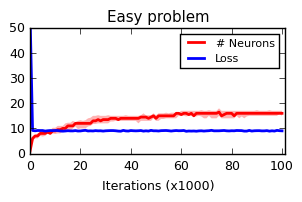
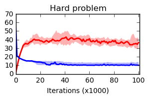
Results are shown in Figure 1. We show both median performance (cross-entropy loss) and median number of neurons as a function of time, over 20 runs. As expected, the hard problem leads to somewhat higher loss than the easy problem. Importantly, the hard problem elicits larger networks than the easy problem (37 neurons vs. 14 neurons after 100000 learning cycles). Thus, the algorithm appropriately allocated more neurons to solve a more difficult task.

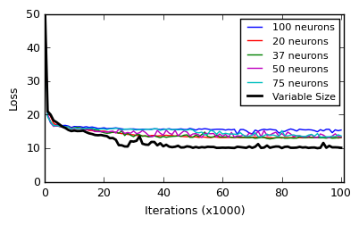
An important question is whether the use of variable-size networks has an impact on performance. We compared the performance of our algorithm against fixed-size networks with various numbers of neurons, ranging from 10 to 100, including one with the same network size as was eventually preferred by our algorithm (i.e. 37 neurons). Results are shown in figure 2, again showing the median loss among 20 runs as a function of time. Intriguingly, the variable-size network actually outperforms fixed-size networks of any size. This result may reflect the advantages of “augmenting topologies” (starting with a minimal network and only adding complexity as needed), as expounded in NEAT [3], at least for the simple problems tackled here.

IV-B Dynamical adjustment of network size in response to changing conditions

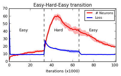
What happens if task difficulty suddenly changes? We tested our network by switching from the “easy” to the “hard” sequence after 33000 cycles, and then back again to the “easy” sequence after 66000 cycles. Results are shown in Figure 3. Interestingly, the network successfully handles the abrupt complexification of the problem by allocating more neurons. Following a large increase, the network then sheds off excess neurons, without damaging performance. This process continues when the problem switches back to the “easy” sequence (note that performance quickly returns to optimal levels). Thus, the network successfully adapts its size to the complexity of the problem at hand.

Figure 2: Comparison of performance for variable and fixed size, for the “hard” problem. The thick black line shows variable-size network performance and is identical to the blue curve in Fig. 1, right panel. Thin colored curves indicate performance of fixed-size networks of various sizes. Curves show medians over 20 runs; inter-quartile ranges (not shown for clarity) are comparable to those seen in Fig. 1. Variable-size networks outperform fixed-size networks for the problem described here.

Figure 3: Dynamic adjustment of network size in response to abrupt complexification and simplification of an ongoing task.

V Conclusions and future work

We have described a method through which the size of a recurrent network can be modified by gradient descent. The method described here can successfully build networks of appropriate size to handle simple problems. This simple method immediately suggests several alternatives and possible extensions.

For example, deletion of neurons could be biased by neuron “age” (i.e. how long the neuron has been present), rather than being random. Deleted neurons could be partially preserved, so that newly added neurons could actually inherit connectivity of previously deleted ones, rather than being randomly initialized. Such adaptations were not necessary for the problems considered here, but might be considered in future applications to more challenging tasks.

The method described here extends naturally to layered feedforward networks. Within each layer, the method can be applied essentially unchanged to adjust layer size. The number of layers can also be made differentiable, by adding and deleting residual layers [1] with initially low pre-additive output weights. These residual layers, which would initially have minimal impact on the network’s output, would play the same role as sub-threshold neurons in the method described above. Similarly, by considering each layer as a higher-order “node”, subject to a global outgoing norm penalty, the method described above could in principle be extended to arbitrary networks composed of multiple areas, with arbitrary connectivity between areas. Further work is needed to assess the practicality of these and other possible extensions.

References

- [1] Kaiming He, Xiangyu Zhang, Shaoqing Ren and Jian Sun “Deep Residual Learning for Image Recognition”, 2015 arXiv:1512.03385 [cs.CV]
- [2] Bruno A Olshausen and David J Field “Emergence of simple-cell receptive field properties by learning a sparse code for natural images” In Nature 381.6583, 1996, pp. 607–609
- [3] Kenneth O Stanley and Risto Miikkulainen “Evolving neural networks through augmenting topologies” In Evol. Comput. 10.2, 2002, pp. 99–127
- [4] Daniel L K Yamins et al. “Performance-optimized hierarchical models predict neural responses in higher visual cortex” In Proc. Natl. Acad. Sci. U. S. A. 111.23, 2014, pp. 8619–8624