Scheme variations of the QCD coupling and hadronic $\tau$ decays

Abstract

The Quantum Chromodynamics (QCD) coupling, $\alpha_{s}$, is not a physical observable of the theory since it depends on conventions related to the renormalization procedure. We introduce a definition of the QCD coupling, denoted by $\widehat{\alpha}_{s}$, whose running is explicitly renormalization scheme invariant. The scheme dependence of the new coupling $\widehat{\alpha}_{s}$ is parameterized by a single parameter $C$, related to transformations of the QCD scale $\Lambda$. It is demonstrated that appropriate choices of $C$ can lead to substantial improvements in the perturbative prediction of physical observables. As phenomenological applications, we study $e^{+}e^{-}$ scattering and decays of the $\tau$ lepton into hadrons, both being governed by the QCD Adler function.

Perturbation theory in the strong coupling, $\alpha_{s}$, is one of the central approaches to predictions in Quantum Chromodynamics (QCD). Because of confinement, however, $\alpha_{s}$ is not a physical observable: its definition inherently depends on theoretical conventions such as renormalization scale and renormalization scheme. Obviously, measurable quantities should not depend on such choices. Regarding the renormalization scale, this independence condition allows to derive so-called renormalization group equations (RGE) which have to be satisfied by all physical quantities. For the renormalization scheme, the situation is more complicated, because order by order the strong coupling can be redefined. For that reason, perturbative computations are performed mainly in convenient schemes like minimal subtraction (MS) ’t Hooft and Veltman (1972) or modified minimal subtraction (${\overline{\rm MS}}$) Bardeen et al. (1978).

The aim of this work is to introduce a new definition of the strong coupling, $\widehat{\alpha}_{s}$, that satisfies two properties. First, the scale running of the coupling, described by the $\beta$-function, is explicitly scheme invariant. Second, the scheme dependence of the coupling can be parameterized by a single parameter $C$. Hence, in the following, we shall refer to this scheme as the $C$-scheme, even though we are actually considering a whole class of schemes. Variations of $C$ will directly correspond to transformations of the QCD scale parameter $\Lambda$.

We then proceed to apply our coupling definition to concrete cases. Among the best studied QCD quantities to which the $C$-scheme may be applied is the two-point vector correlator and the related Adler function Adler (1974), which emerge in calculations of the total cross section of $e^{+}e^{-}$ scattering into hadrons, and that also govern theoretical predictions of the inclusive decay rate of $\tau$ leptons into hadronic final states Braaten et al. (1992). At present, their perturbative expansion is known up to the fourth order in $\alpha_{s}$ Baikov et al. (2008). Having at our disposal a parameter to investigate scheme variations, we show that appropriate choices of $C$ can lead to substantial improvements in the predictions for these quantities. The use of $\widehat{\alpha}_{s}$ for the scalar correlator, which is relevant for the prediction of Higgs boson decay into quarks and for light quark-mass determinations from QCD sum rules, is investigated in a related article Jamin and Miravitllas .

Compared to other celebrated methods used for the optimization of perturbative predictions, the procedure we present here differs in more than one way. The main difference is that we seek to optimize the perturbative prediction by exploiting its scheme dependence, while the idea behind methods such as BLM Brodsky et al. (1983) or PMC Brodsky and Wu (2012); Mojaza et al. (2013) is to obtain a scheme-independent result through a well defined algorithm for setting the renormalization scale, regardless of the intermediate scheme used for the perturbative calculation (which most often is ${\overline{\rm MS}}$). Furthermore, some of these methods, such as for example the “effective charge” Grunberg (1984), involve a process dependent definition of the coupling. In the procedure described here, one defines a process independent class of schemes, parameterized by a single continuous parameter $C$. We then explore variations of this parameter in order to optimize the perturbative series in the spirit of asymptotic expansions. This, however, entails that preferred values of the parameter $C$ depend on the process considered.

Let us begin with the scale running of the QCD coupling $\alpha_{s}$, which is described by the $\beta$-function as

$$-\,Q\,\frac{{\rm d}a_{Q}}{{\rm d}Q}\,\equiv\,\beta(a_{Q})\,=\,\beta_{1}\,a_{Q}^{2}+\beta_{2}\,a_{Q}^{3}+\beta_{3}\,a_{Q}^{4}+\ldots\,.$$ (1)

Here and in the following, $a_{Q}\equiv\alpha_{s}(Q)/\pi$, $Q$ is a physically relevant scale, and the first five $\beta$-coefficients $\beta_{1}$ to $\beta_{5}$ are analytically available van Ritbergen et al. (1997); Baikov et al. (2016). (In our conventions, they have been collected in Appendix A of Ref. Jamin and Miravitllas .)

Employing the RGE (1) for $a_{Q}$, the well-known scale-invariant QCD parameter $\Lambda$ can be defined by

$$\Lambda\,\equiv\,Q\,{\rm e}^{-\frac{1}{\beta_{1}a_{Q}}}\,[a_{Q}]^{-\frac{\beta_{2}}{\beta_{1}^{2}}}\exp\Biggl{\{}\,\int\limits_{0}^{a_{Q}}\,\frac{{\rm d}a}{\tilde{\beta}(a)}\Biggr{\}}\,,$$ (2)

where

$$\frac{1}{\tilde{\beta}(a)}\,\equiv\,\frac{1}{\beta(a)}-\frac{1}{\beta_{1}a^{2}}+\frac{\beta_{2}}{\beta_{1}^{2}a}\,,$$ (3)

which is free of singularities in the limit $a\to 0$. Let us consider a scheme transformation to a new coupling $a^{\prime}$, which takes the general form

$$a^{\prime}\,\equiv\,a+c_{1}\,a^{2}+c_{2}\,a^{3}+c_{3}\,a^{4}+\ldots\,.$$ (4)

The $\Lambda$-parameter in the new scheme, $\Lambda^{\prime}$, only depends on $c_{1}$ and not on the remaining higher-order coefficients. The precise relation reads Celmaster and Gonsalves (1979)

$$\Lambda^{\prime}\,=\,\Lambda\,{\rm e}^{c_{1}/\beta_{1}}\,.$$ (5)

The fact that redefinitions of the $\Lambda$-parameter only involve a single constant motivates the implicit definition of a new coupling $\hat{a}_{Q}$, which is scheme invariant, except for shifts in $\Lambda$, parameterized by a parameter $C$:

$$\frac{1}{\hat{a}_{Q}}+\frac{\beta_{2}}{\beta_{1}}\ln\hat{a}_{Q}\, \equiv \,\beta_{1}\Big{(}\ln\frac{Q}{\Lambda}+\frac{C}{2}\Big{)}$$ (6)

$$\,=\,\frac{1}{a_{Q}}+\frac{\beta_{1}}{2}\,C+\frac{\beta_{2}}{\beta_{1}}\ln a_{Q}-\beta_{1}\!\int\limits_{0}^{a_{Q}}\,\frac{{\rm d}a}{\tilde{\beta}(a)}\,.$$

In perturbation theory, Eq. (6) should be interpreted in an iterative sense. Evidently, $\hat{a}_{Q}$ is a function of $C$ but, for notational simplicity, we will not make this dependence explicit. One should remark that a combination similar to (6), but without the logarithmic term on the left-hand side, was already discussed in Refs. Brown et al. (1992); Beneke (1993). However, without this term, an unwelcome logarithm of $a_{Q}$ remains in the perturbative relation between the couplings $\hat{a}_{Q}$ and $a_{Q}$. This non-analytic term is avoided by the construction of Eq. (6).

In Fig. 1, we display the coupling $\hat{a}$ according to Eq. (6) as a function of $C$. Since in this letter we focus on hadronic $\tau$ decays, as our initial ${\overline{\rm MS}}$ input we employ $\alpha_{s}(M_{\tau})=0.316(10)$, which results from the current PDG average $\alpha_{s}(M_{Z})=0.1181(13)$ Olive et al. (2014). The yellow band corresponds to the variation within the $\alpha_{s}$ uncertainties. Below roughly $C=-2$, the relation between $\hat{a}$ and the ${\overline{\rm MS}}$ coupling ceases to be perturbative and breaks down.

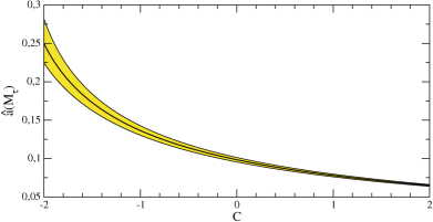
Figure 1: The coupling $\hat{a}(M_{\tau})$ according to Eq. (6) as a function of $C$, and for the ${\overline{\rm MS}}$ input value $\alpha_{s}(M_{\tau})=0.316(10)$. The yellow band corresponds to the $\alpha_{s}$ uncertainty.

The perturbative relations between the coupling $\hat{a}$ and $a$ in a particular scheme can straightforwardly be deduced from Eq. (6). Taking $a$ as well as the corresponding $\beta$-function coefficients in the ${\overline{\rm MS}}$ scheme, and for three quark flavors, $N_{f}=3$, the expansions read,

$$\hat{a}(a)\, = \,a-\mbox{$\frac{9}{4}$}\,C\,a^{2}-\big{(}\mbox{$\frac{3397}{2592}$}+4C-\mbox{$\frac{81}{16}$}\,C^{2}\big{)}a^{3}-\big{(}\mbox{$\frac{741103}{186624}$}$$

$$+\,\mbox{$\frac{233}{192}$}\,C-\mbox{$\frac{45}{2}$}\,C^{2}+\mbox{$\frac{729}{64}$}\,C^{3}+\mbox{$\frac{445}{144}$}\zeta_{3}\big{)}a^{4}-\big{(}\mbox{$\frac{727240925}{80621568}$}$$

$$-\,\mbox{$\frac{869039}{41472}$}\,C-\mbox{$\frac{26673}{512}$}\,C^{2}+\mbox{$\frac{351}{4}$}\,C^{3}-\mbox{$\frac{6561}{256}$}\,C^{4}-\mbox{$\frac{445}{32}$}\zeta_{3}C$$

$$+\,\mbox{$\frac{10375693}{373248}$}\zeta_{3}-\mbox{$\frac{1335}{256}$}\zeta_{4}-\mbox{$\frac{534385}{20736}$}\zeta_{5}\big{)}a^{5}+{\cal O}(a^{6})\,,$$ (7)

and

$$a(\hat{a})\, = \,\hat{a}+\mbox{$\frac{9}{4}$}\,C\,\hat{a}^{2}+\big{(}\mbox{$\frac{3397}{2592}$}+4C+\mbox{$\frac{81}{16}$}\,C^{2}\big{)}\hat{a}^{3}+\big{(}\mbox{$\frac{741103}{186624}$}$$

$$+\,\mbox{$\frac{18383}{1152}$}\,C+\mbox{$\frac{45}{2}$}\,C^{2}+\mbox{$\frac{729}{64}$}\,C^{3}+\mbox{$\frac{445}{144}$}\zeta_{3}\big{)}\hat{a}^{4}+\big{(}\mbox{$\frac{1142666849}{80621568}$}$$

$$+\,\mbox{$\frac{1329359}{20736}$}\,C+\mbox{$\frac{28623}{256}$}\,C^{2}+\mbox{$\frac{351}{4}$}\,C^{3}+\mbox{$\frac{6561}{256}$}\,C^{4}+\mbox{$\frac{445}{16}$}\zeta_{3}C$$

$$+\,\mbox{$\frac{10375693}{373248}$}\zeta_{3}-\mbox{$\frac{1335}{256}$}\zeta_{4}-\mbox{$\frac{534385}{20736}$}\zeta_{5}\big{)}\hat{a}^{5}+{\cal O}(\hat{a}^{6})\,,$$ (8)

where $\zeta_{i}\equiv\zeta(i)$ stands for the Riemann $\zeta$-function.

The running of the coupling $\hat{a}$ can also be deduced from Eq. (6). To this end, one first has to derive its $\beta$-function which is found to have the simple form

$$-\,Q\,\frac{{\rm d}\hat{a}_{Q}}{{\rm d}Q}\,\equiv\,\hat{\beta}(\hat{a}_{Q})\,=\,\frac{\beta_{1}\hat{a}_{Q}^{2}}{\left(1-\mbox{$\frac{\beta_{2}}{\beta_{1}}$}\,\hat{a}_{Q}\right)}\,.$$ (9)

As is seen explicitly, it only depends on the scheme-invariant $\beta$-function coefficients $\beta_{1}$ and $\beta_{2}$. It may also be remarked that the only non-trivial zero of $\hat{\beta}(\hat{a})$ arises in the case of $\beta_{1}=0$. Integrating the RGE (9) yields

$$\frac{1}{\hat{a}_{Q}}\,=\,\frac{1}{\hat{a}_{\mu}}+\frac{\beta_{1}}{2}\ln\frac{Q^{2}}{\mu^{2}}-\frac{\beta_{2}}{\beta_{1}}\ln\frac{\hat{a}_{Q}}{\hat{a}_{\mu}}\,.$$ (10)

Again, this implicit equation for $\hat{a}_{Q}$ can either be solved iteratively, to provide a perturbative expansion, or numerically.

As our first application of the coupling $\widehat{\alpha}_{s}$, we investigate the perturbative series of the Adler function, $D(a_{Q})$ Adler (1974); Baikov et al. (2008). To this end, it is convenient to define the reduced Adler function $\widehat{D}(a_{Q})$ as

$$4\pi^{2}D(a_{Q})-1\, \equiv \,\widehat{D}(a_{Q})\,=\,\sum_{n=1}^{\infty}c_{n,1}a_{Q}^{n}$$ (11)

$$\,=\,a_{Q}+1.640\,a_{Q}^{2}+6.371\,a_{Q}^{3}+49.08\,a_{Q}^{4}+\ldots$$

We adopt the notation of Ref. Beneke and Jamin (2008), with numerical coefficients in the ${\overline{\rm MS}}$ scheme and for $N_{f}=3$. The renormalization scale logarithms $\ln(Q/\mu)$ appearing in the Adler function have been resummed with the choice $\mu=Q$.

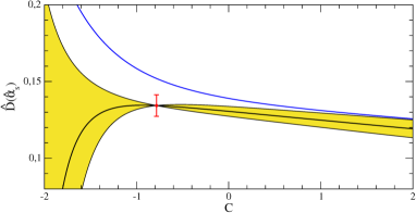
Figure 2: $\widehat{D}(\hat{a}_{M_{\tau}})$ of Eq. (Scheme variations of the QCD coupling and hadronic $\tau$ decays) as a function of $C$. The yellow band arises from either removing or doubling the fifth-order term. In the red dot, the ${\cal O}(\hat{a}^{5})$ vanishes, and ${\cal O}(\hat{a}^{4})$ is taken as the uncertainty. For further explanation, see the text.

Using the relation (Scheme variations of the QCD coupling and hadronic $\tau$ decays), we rewrite the expansion (11) for $\widehat{D}$ in terms of the $C$-scheme coupling $\hat{a}_{Q}$, resulting in

$$\widehat{D}(\hat{a}_{Q})\, = \,\hat{a}_{Q}+(1.640+2.25C)\,\hat{a}_{Q}^{2}$$

$$+\,(7.682+11.38C+5.063C^{2})\,\hat{a}_{Q}^{3}$$ (12)

$$+\,(61.06+72.08C+47.40C^{2}+11.39C^{3})\,\hat{a}_{Q}^{4}+\ldots$$

A graphical representation of Eq. (Scheme variations of the QCD coupling and hadronic $\tau$ decays) is provided in Fig. 2, where $\widehat{D}(\hat{a}_{M_{\tau}})$ is plotted as a function of $C$. The yellow band this time corresponds to an error estimate from the fifth-order contribution. The required coefficient has been taken to be $c_{5,1}=283$, as estimated in Ref. Beneke and Jamin (2008). The yellow band then arises by either removing or doubling the ${\cal O}(\hat{a}^{5})$ term. Generally, it is observed that around $C\!\approx\!-1$, a region of stability with respect to the $C$-variation emerges. For comparison, the blue line corresponds to using $c_{5,1}=566$ and still doubling the ${\cal O}(\hat{a}^{5})$ correction. Then, no region of stability is found which seems to indicate that such large values of $c_{5,1}$ are disfavored. In the red dot, where $C=-0.783$, the ${\cal O}(\hat{a}^{5})$ vanishes, and the ${\cal O}(\hat{a}^{4})$ correction, which is the last included non-vanishing term, has been employed as a conservative uncertainty, in the spirit of asymptotic expansions. Numerically, we find

$$\widehat{D}(\hat{a}_{M_{\tau}},C=-0.783)\,=\,0.1343\pm 0.0070\pm 0.0067\,,$$ (13)

where the second error originates from the uncertainty in $\alpha_{s}(M_{\tau})$. The result (13) may be compared to the direct ${\overline{\rm MS}}$ prediction (11), which reads

$$\widehat{D}(a_{M_{\tau}})\,=\,0.1316\pm 0.0029\pm 0.0060\,.$$ (14)

Here, the first error is obtained by removing or doubling $c_{5,1}$, and the second error again corresponds to the $\alpha_{s}$ uncertainty.

A final comparison of (13) and (14) may be performed with the Adler function model that was put forward in Ref. Beneke and Jamin (2008), and which is based on general knowledge of the renormalon structure for the Borel transform of $\widehat{D}(a_{Q})$. Within this model, one obtains

$$\widehat{D}(a_{M_{\tau}})\,=\,0.1354\pm 0.0127\pm 0.0058\,.$$ (15)

In this case, the first uncertainty results from estimates of the perturbative ambiguity that arises from the renormalon singularities. It is seen that this uncertainty is much bigger than the one of (14) and still larger than the one of (13). Therefore, we conclude that the higher-order uncertainty of (14) appears to be underestimated, while Eq. (13) seems to provide a more realistic account of the resummed series. Interestingly enough, also its central value is closer to the Borel model result.

Now, we turn to the perturbative expansion for the total $\tau$ hadronic width. The central observable is the ratio $R_{\tau}$ of the total hadronic branching fraction to the electron branching fraction. It can be parameterized as

$$R_{\tau}\,=\,3\,S_{\rm EW}(|V_{ud}|^{2}+|V_{us}|^{2})\,(1+\delta^{(0)}+\cdots)\,,$$ (16)

where $S_{\rm EW}$ is an electroweak correction and $V_{ud}$ as well as $V_{us}$ CKM matrix elements. Perturbative QCD is encoded in $\delta^{(0)}$ (see Refs. Braaten et al. (1992); Beneke and Jamin (2008) for details) and the ellipsis indicate further small subleading corrections. For $\delta^{(0)}$ a complication arises, because it is calculated from a contour integral in the complex energy plane. On the other hand, we seek to resum the scale logarithms $\ln(Q/\mu)$, and the perturbative prediction depends on whether those logs are resummed before or after performing the contour integration. The first choice is called contour-improved perturbation theory (CIPT) Diberder and Pich (1992) and the second fixed-order perturbation theory (FOPT).

In FOPT, the perturbative series of $\delta^{(0)}(a_{Q})$ in terms of the ${\overline{\rm MS}}$ coupling $a_{Q}$ is given by Baikov et al. (2008); Beneke and Jamin (2008)

$$\delta_{\rm FO}^{(0)}(a_{Q})\,=\,a_{Q}+5.202\,a_{Q}^{2}+26.37\,a_{Q}^{3}+127.1\,a_{Q}^{4}+\ldots$$ (17)

On the other hand, in the $C$-scheme coupling $\hat{a}_{Q}$, the expansion for $\delta^{(0)}(\hat{a}_{Q})$ reads

$$\delta_{\rm FO}^{(0)}(\hat{a}_{Q})\, = \,\hat{a}_{Q}+(5.202+2.25C)\,\hat{a}_{Q}^{2}$$

$$+\,(27.68+27.41C+5.063C^{2})\,\hat{a}_{Q}^{3}$$ (18)

$$+\,(148.4+235.5C+101.5C^{2}+11.39C^{3})\,\hat{a}_{Q}^{4}+\ldots$$

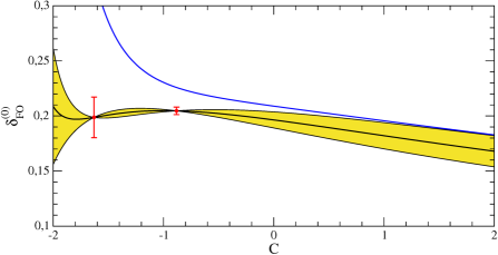
Figure 3: $\delta_{\rm FO}^{(0)}(\hat{a}_{Q})$ of Eq. (Scheme variations of the QCD coupling and hadronic $\tau$ decays) as a function of $C$. The yellow band arises from either removing or doubling the fifth-order term. In the red dots, the ${\cal O}(\hat{a}^{5})$ vanishes, and ${\cal O}(\hat{a}^{4})$ is taken as the uncertainty. For further explanation, see the text.

In Fig. 3, we display $\delta_{\rm FO}^{(0)}(\hat{a}_{Q})$ as a function of $C$. Assuming $c_{5,1}=283$, the yellow band again corresponds to removing or doubling the ${\cal O}(\hat{a}^{5})$ term. Like for $\widehat{D}(\hat{a})$, a nice plateau is found for $C\approx-1$. Taking $c_{5,1}=566$ and then doubling the ${\cal O}(\hat{a}^{5})$ results in the blue curve that does not show stability. Hence, this scenario again is disfavored. In the red dots, which lie at $C=-0.882$ and $C=-1.629$, the ${\cal O}(\hat{a}^{5})$ correction vanishes, and the ${\cal O}(\hat{a}^{4})$ term is taken as the uncertainty. The point to the right has a substantially smaller error, and yields

$$\delta_{\rm FO}^{(0)}(\hat{a}_{M_{\tau}},C=-0.882)\,=\,0.2047\pm 0.0034\pm 0.0133\,.$$ (19)

Once more, the second error covers the uncertainty of $\alpha_{s}(M_{\tau})$. In this case, the direct ${\overline{\rm MS}}$ prediction of Eq. (17) is found to be

$$\delta_{\rm FO}^{(0)}(a_{M_{\tau}})\,=\,0.1991\pm 0.0061\pm 0.0119\,.$$ (20)

This value is somewhat lower, but within $1\,\sigma$ of the higher-order uncertainty. Comparing, on the other hand, to the Borel model (BM) result of Beneke and Jamin (2008), which is given by

$$\delta_{\rm BM}^{(0)}(a_{M_{\tau}})\,=\,0.2047\pm 0.0029\pm 0.0130\,,$$ (21)

it is found that (19) and (21) are surprisingly similar. In both cases, the parametric $\alpha_{s}$ uncertainty is substantially larger than the higher-order one – especially given the recent increase in the $\alpha_{s}$ uncertainty provided by the PDG Olive et al. (2014) – which underlines the good potential of $\alpha_{s}$ extractions from hadronic $\tau$ decays.

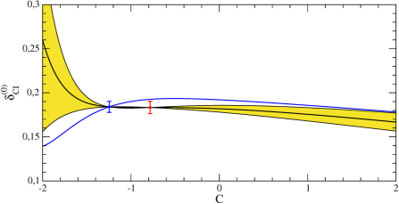
Figure 4: $\delta_{\rm CI}^{(0)}(\hat{a}_{Q})$ as a function of $C$. The yellow band arises from either removing or doubling the fifth-order term. In the red and blue dots, the ${\cal O}(\hat{a}^{5})$ vanishes, and ${\cal O}(\hat{a}^{4})$ is taken as the uncertainty. For further explanation, see the text.

In CIPT, contour integrals over the running coupling, Eq. (10), have to be computed, and hence the result cannot be given in analytical form. Graphically, $\delta_{\rm CI}^{(0)}(a_{M_{\tau}})$ as a function of $C$ is displayed in Fig. 4. The general behavior is very similar to FOPT, with the exception that now also for $c_{5,1}=566$ a zero of the ${\cal O}(\hat{a}^{5})$ term is found. This time, both zeros have similar uncertainties, and employing the point with smaller error (in blue) yields

$$\delta_{\rm CI}^{(0)}(\hat{a}_{M_{\tau}},C=-1.246)\,=\,0.1840\pm 0.0062\pm 0.0084\,.$$ (22)

As has been discussed many times in the past (see e.g. Beneke and Jamin (2008)) the CIPT prediction lies substantially below the FOPT results, especially the $C$-scheme ones, and the Borel model. On the other hand, the parametric $\alpha_{s}$ uncertainty in CIPT turns out to be smaller.

In this work, in Eq. (6), we have defined a class of QCD couplings $\hat{a}_{Q}$, such that the scale running is explicitly scheme invariant, and scheme changes are parameterized by a single constant $C$. For this reason, we have termed $\hat{a}_{Q}$ the $C$-scheme coupling. Scheme transformations correspond to changes in the QCD scale $\Lambda$.

We have applied the coupling $\hat{a}_{Q}$ to investigations of the perturbative series of the reduced Adler function $\widehat{D}$. Our central result is given in Eq. (13). Its higher-order uncertainty turned out larger than the corresponding ${\overline{\rm MS}}$ prediction (14), but we consider (13) to be more realistic and conservative.

We also studied the perturbative expansion of the $\tau$ hadronic width, employing the coupling $\hat{a}_{Q}$. In this case our central prediction in FOPT is given in Eq. (19). Surprisingly, the result (19) is found very close to the prediction (21) of the central Borel model developed in Ref. Beneke and Jamin (2008), hence providing some support for this approach.

The disparity between FOPT and CIPT predictions for $\delta^{(0)}$ is not resolved by the $C$-scheme. As is seen from Eq. (22), the CIPT result turns out substantially lower (as is the case for the ${\overline{\rm MS}}$ prediction). This suggests to return to investigations of Borel models, this time in the coupling $\hat{a}$, in order to assess the scheme dependence of such models. This could result in an improved extraction of $\alpha_{s}$ from hadronic decays of the $\tau$ lepton.