Scalar correlator, Higgs decay into quarks, and scheme variations of the QCD coupling

Abstract

In this work, the perturbative QCD series of the scalar correlation function $\Psi(s)$ is investigated. Besides $\mbox{\rm Im}\Psi(s)$, which is relevant for Higgs decay into quarks, two other physical correlators, $\Psi^{{}^{\prime\prime}}(s)$ and $D^{L}(s)$, have been employed in QCD applications like quark mass determinations or hadronic $\tau$ decays. $D^{L}(s)$ suffers from large higher-order corrections and, by resorting to the large-$\beta_{0}$ approximation, it is shown that this is related to a spurious renormalon ambiguity at $u=1$. Hence, this correlator should be avoided in phenomenological analyses. Moreover, it turns out advantageous to express the quark mass factor, introduced to make the scalar current renormalisation group invariant, in terms of the renormalisation invariant quark mass $\widehat{m}_{q}$. To further study the behaviour of the perturbative expansion, we introduce a QCD coupling $\widehat{\alpha}_{s}$, whose running is explicitly renormalisation scheme independent. The scheme dependence of $\widehat{\alpha}_{s}$ is parametrised by a single parameter $C$, being related to transformations of the QCD scale parameter $\Lambda$. It is demonstrated that appropriate choices of $C$ lead to a substantial improvement in the behaviour of the perturbative series for $\Psi^{{}^{\prime\prime}}(s)$ and $\mbox{\rm Im}\Psi(s)$.

1 Introduction

The scalar correlation function in QCD plays an important role, as it governs the decay of the Higgs into quark-antiquark pairs, and it has been employed in determinations of quark masses from QCD sum rules as well as hadronic decays of the $\tau$ lepton. Presently, the perturbative expansion for the scalar correlator is known analytically up to order $\alpha_{s}^{4}$ in the strong coupling bck05 ; che96 ; gkls90 , and estimates of the next, fifth order have been attempted in the literature. While the decay of the Higgs boson into quark-antiquark pairs is connected to the imaginary part of the scalar correlator $\Psi(s)$ djou08 , two other physical correlators, $\Psi^{{}^{\prime\prime}}(s)$ and $D^{L}(s)$, have been utilised in QCD sum rule analyses, the former in quark mass extractions jop02 ; jop06 and the latter in hadronic $\tau$ decays pp98 ; pp99 ; gjpps03 . In this work we shall investigate the perturbative series of all three.

In order to achieve reliable error estimates of missing higher orders in QCD predictions, a better understanding of the perturbative behaviour of the scalar correlator at high orders is desirable. Work along those lines has been performed in ref. bkm00 , where the scalar correlation function has been calculated in the large-$N_{f}$ approximation ben92 ; bro92 , or relatedly the large-$\beta_{0}$ approximation bb94 (for a review see ben98 ), to all orders in the strong coupling. However, as will be discussed in more detail below, the large-$\beta_{0}$ approximation does not provide a satisfactory representation of the scalar correlator in full QCD. Still, as will be demonstrated, it can serve as a guideline to shed light on the general structure of the scalar correlation function.

Furthermore, while large QCD corrections are found in the case of the correlator $D^{L}(s)$, the corrections are substantially smaller for $\mbox{\rm Im}\Psi(s)$ and $\Psi^{{}^{\prime\prime}}(s)$. In the large-$\beta_{0}$ approximation this observation can be traced back to the presence of a spurious renormalon pole in the Borel transform at $u=1$ for $D^{L}(s)$, whereas $\Psi^{{}^{\prime\prime}}(s)$ and $\mbox{\rm Im}\Psi(s)$ are free from this contribution. We discuss the origin of the additional renormalon pole and its implications, but at any rate conclude that, in view of this fact, the correlator $D^{L}(s)$ should be avoided in phenomenological analyses.

Additionally, the large-$\beta_{0}$ approximation motivates a strategy in order to improve the perturbative expansion. The structure of the Borel transform in the large-$\beta_{0}$ limit suggests the introduction of a renormalisation scheme invariant QCD coupling $\widehat{\alpha}_{s}$, which underlines the scheme invariance of the perturbative term for the physical quantities under investigation. In fact, all contributions of infrared (IR) and ultraviolet (UV) renormalons individually are scheme independent. It is then found that higher-order corrections tend to become smaller when re-expressing the perturbative series in terms of the coupling $\widehat{\alpha}_{s}$. One reason for this behaviour appears to be that part of the perturbative corrections are resummed into a global prefactor $\alpha_{s}^{\delta}$ which is present for the scalar correlator.

In full QCD, the construction of a scheme-invariant coupling does not appear to be possible, at least in a universal sense, independent of any observable. Nonetheless, we are able to provide the definition of a QCD coupling, which we also term $\widehat{\alpha}_{s}$, and whose running is scheme independent and described by a simple $\beta$-function, only depending on the coefficients $\beta_{1}$ and $\beta_{2}$. Different schemes can then be parametrised by a single parameter $C$, which corresponds to transformations of the QCD scale parameter $\Lambda$. By investigating two phenomenological applications, the correlator $\Psi^{{}^{\prime\prime}}(s)$ at the $\tau$ mass scale and $\mbox{\rm Im}\Psi(s)$ for Higgs decay to quarks, we show that employing the coupling $\widehat{\alpha}_{s}$ and choosing appropriate schemes by varying the parameter $C$, the behaviour of the perturbative series can be substantially improved.

Our article is organised as follows: in section 2, theoretical expressions for the scalar correlation function $\Psi(s)$ and the corresponding physical correlators $\mbox{\rm Im}\Psi(s)$, $\Psi^{{}^{\prime\prime}}(s)$ and $D^{L}(s)$ are collected, and the present knowledge on the perturbative expansions is summarised. Furthermore, the renormalisation group invariant quark mass $\widehat{m}_{q}$ is introduced, and the correlators are rewritten in terms of this mass definition. In section 3, we review the results of ref. bkm00 on the scalar correlation function in the large-$\beta_{0}$ approximation and apply them to a discussion of the correlators $\Psi^{{}^{\prime\prime}}(s)$ and $D^{L}(s)$. Next, in section 4, we define the coupling $\widehat{\alpha}_{s}$, and compute its $\beta$-function as well as the perturbative relation to $\alpha_{s}$ in the ${\overline{\rm MS}}$ scheme. Finally, in section 5, two phenomenological applications, $\Psi^{{}^{\prime\prime}}(s)$ at the $\tau$ mass scale and $\mbox{\rm Im}\Psi(s)$ for Higgs decay, are investigated, and followed by our conclusions in section 6. More technical material like the coefficients of the renormalisation group functions, higher-order coefficients relevant for the large-$\beta_{0}$ approximation, as well as a discussion of the subtraction constant $\Psi(0)$, are relegated to appendices.

2 The scalar two-point correlator

The following work shall be concerned with the scalar two-point correlation function $\Psi(p^{2})$ which is defined by

$$\Psi(p^{2})\,\equiv\,i\!\int\!{\rm d}x\,{\rm e}^{ipx}\langle\Omega|T\{j(x)j^{\dagger}(0)\}|\Omega\rangle\,.$$ (1)

The non-perturbative, full QCD vacuum is denoted by $|\Omega\rangle$. For our two applications, the scalar current $j(x)$ is chosen to arise either from the divergence of the normal-ordered vector current,

$$j(x)\,=\,\partial^{\mu}\!:\!\bar{u}(x)\gamma_{\mu}s(x)\!:\;=\,i\,(m_{u}-m_{s})\!:\!\bar{u}(x)s(x)\!:\,,$$ (2)

or the interaction of the Higgs boson with quarks,

$$j(x)\,=\,m_{q}\!:\!\bar{q}(x)q(x)\!:.$$ (3)

These choices have the advantage of an additional factor of the quark masses, which makes the currents $j(x)$ renormalisation group invariant (RGI). Furthermore, the first current is taken to be flavour non-diagonal, with a particular flavour content that plays a role in hadronic $\tau$ decays to strange final states.

The purely perturbative expansion of $\Psi(p^{2})$ is known up to order $\alpha_{s}^{4}$ bck05 and takes the general form

$$\Psi_{\rm PT}(s)\,=\,-\,\frac{N_{c}}{8\pi^{2}}\,m_{\mu}^{2}\,s\sum\limits_{n=0}^{\infty}a_{\mu}^{n}\sum\limits_{k=0}^{n+1}d_{n,k}L^{k}\,,$$ (4)

where $s\equiv p^{2}$ and $a_{\mu}\equiv\alpha_{s}(\mu)/\pi$. To simplify the notation, we have introduced the generic mass factor $m_{\mu}$ which either stands for the combination $(m_{u}(\mu)-m_{s}(\mu))$ or $m_{q}(\mu)$. The running quark masses and the QCD coupling are renormalised at the scale $\mu$, which enters in $L\equiv\ln(-s/\mu^{2})$. As a matter of principle, different scales could be introduced for the renormalisation of coupling and quark masses, but for simplicity, we refrain from this choice. Below, this option will, however, be discussed in relation to renormalisation schemes.

At each perturbative order $n$, the only independent coefficients $d_{n,k}$ are the $d_{n,1}$. The coefficients $d_{n,0}$ depend on the renormalisation prescription and do not contribute in physical quantities, while all remaining coefficients $d_{n,k}$ with $k>1$ can be obtained by means of the renormalisation group equation (RGE). The normalisation in eq. (4) is chosen such that $d_{0,1}=1$. Setting the number of colours $N_{c}=3$, and employing the ${\overline{\rm MS}}$-scheme bbdm78 , after tremendous efforts the coefficients $d_{n,1}$ up to ${\cal O}(\alpha_{s}^{4})$ were found to be gkls90 ; che96 ; bck05 :

$$d_{0,1}\,=\,1\,,\qquad d_{1,1}\,=\,\mbox{$\frac{17}{3}$}\,,\qquad d_{2,1}\,=\,\mbox{$\frac{10801}{144}$}-\mbox{$\frac{39}{2}$}\zeta_{3}+\Big{(}\!-\mbox{$\frac{65}{24}$}+\mbox{$\frac{2}{3}$}\zeta_{3}\Big{)}N_{f}$$ (5)

$$d_{3,1}\,=\,\mbox{$\frac{6163613}{5184}$}-\mbox{$\frac{109735}{216}$}\zeta_{3}+\mbox{$\frac{815}{12}$}\zeta_{5}+\Big{(}\!-\mbox{$\frac{46147}{486}$}+\mbox{$\frac{262}{9}$}\zeta_{3}-\mbox{$\frac{5}{6}$}\zeta_{4}-\mbox{$\frac{25}{9}$}\zeta_{5}\Big{)}N_{f}+\Big{(}\mbox{$\frac{15511}{11664}$}-\mbox{$\frac{1}{3}$}\zeta_{3}\Big{)}N_{f}^{2}$$

$$d_{4,1} \!=\! \mbox{$\frac{10811054729}{497664}$}-\mbox{$\frac{3887351}{324}$}\zeta_{3}+\mbox{$\frac{458425}{432}$}\zeta_{3}^{2}+\mbox{$\frac{265}{18}$}\zeta_{4}+\mbox{$\frac{373975}{432}$}\zeta_{5}-\mbox{$\frac{1375}{32}$}\zeta_{6}-\mbox{$\frac{178045}{768}$}\zeta_{7}$$

$$+\,\Big{(}\!-\mbox{$\frac{1045811915}{373248}$}+\mbox{$\frac{5747185}{5184}$}\zeta_{3}-\mbox{$\frac{955}{16}$}\zeta_{3}^{2}-\mbox{$\frac{9131}{576}$}\zeta_{4}+\mbox{$\frac{41215}{432}$}\zeta_{5}+\mbox{$\frac{2875}{288}$}\zeta_{6}+\mbox{$\frac{665}{72}$}\zeta_{7}\Big{)}N_{f}$$

$$+\,\Big{(}\mbox{$\frac{220313525}{2239488}$}-\mbox{$\frac{11875}{432}$}\zeta_{3}+\mbox{$\frac{5}{6}$}\zeta_{3}^{2}+\mbox{$\frac{25}{96}$}\zeta_{4}-\mbox{$\frac{5015}{432}$}\zeta_{5}\Big{)}N_{f}^{2}+\Big{(}\!-\mbox{$\frac{520771}{559872}$}+\mbox{$\frac{65}{432}$}\zeta_{3}+\mbox{$\frac{1}{144}$}\zeta_{4}+\mbox{$\frac{5}{18}$}\zeta_{5}\Big{)}N_{f}^{3}\,.$$

For future reference, at $N_{f}=3$, numerically, the respective coefficients take the values

$$d_{1,1}\,=\,5.6667\,,\qquad d_{2,1}\,=\,45.846\,,\qquad d_{3,1}\,=\,465.85\,,\qquad d_{4,1}\,=\,5588.7\,.$$ (6)

The case $N_{f}=5$, relevant for Higgs boson decay, will be considered in the phenomenological applications of section 5.

As indicated above, the correlator $\Psi(s)$ itself is not related to a measurable quantity. Since it grows linearly with $s$ as $s$ tends to infinity, it satisfies a dispersion relation with two subtraction constants,

$$\Psi(s)\,=\,\Psi(0)+s\,\Psi^{{}^{\prime}}(0)+s^{2}\!\int\limits_{0}^{\infty}\!\frac{\rho(s^{\prime})}{(s^{\prime})^{2}(s^{\prime}-s-i0)}\,{\rm d}s^{\prime}\,,$$ (7)

where $\rho(s)\equiv\mbox{\rm Im}\Psi(s+i0)/\pi$ is the scalar spectral function. Hence, a possibility to construct a physical quantity other than the spectral function itself, which will be discussed further down below, is to employ the second derivative of $\Psi(s)$ with respect to $s$. Since the two derivatives remove the two unphysical subtractions, $\Psi^{{}^{\prime\prime}}(s)$ is then only related to the spectral function. The corresponding dispersion relation reads

$$\Psi^{{}^{\prime\prime}}(s)\,=\,2\!\int\limits_{0}^{\infty}\!\frac{\rho(s^{\prime})}{(s^{\prime}-s-i0)^{3}}\,{\rm d}s^{\prime}\,,$$ (8)

and the general perturbative expansion is

$$\Psi_{\rm PT}^{{}^{\prime\prime}}(s)\,=\,-\,\frac{N_{c}}{8\pi^{2}}\,\frac{m_{\mu}^{2}}{s}\,\sum\limits_{n=0}^{\infty}a_{\mu}^{n}\sum\limits_{k=1}^{n+1}d_{n,k}\,k\,\big{[}L^{k-1}+(k-1)L^{k-2}\big{]}\,.$$ (9)

Being a physical quantity, $\Psi^{{}^{\prime\prime}}(s)$ satisfies a homogeneous RGE, and therefore the logarithms can be resummed with the particular scale choice $\mu^{2}=-s\equiv Q^{2}$, leading to the compact expression

$$\Psi_{\rm PT}^{{}^{\prime\prime}}(Q^{2})\,=\,\frac{N_{c}}{8\pi^{2}}\,\frac{m_{Q}^{2}}{Q^{2}}\,\biggl{\{}\,1+\sum\limits_{n=1}^{\infty}\,(d_{n,1}+2d_{n,2})\,a_{Q}^{n}\,\biggr{\}}\,.$$ (10)

In this way, both the running quark mass as well as the running QCD coupling are to be evaluated at the renormalisation scale $Q$. The dependent coefficients $d_{n,2}$ can be calculated from the RGE. They are collected in appendix A, together with the coefficients of the QCD $\beta$-function and mass anomalous dimension. Numerically, at $N_{f}=3$, the perturbative coefficients $d_{n,1}^{\,{}^{\prime\prime}}\equiv d_{n,1}+2d_{n,2}$ of eq. (10) take the values

$$d_{1,1}^{\,{}^{\prime\prime}}\,=\,3.6667\,,\qquad d_{2,1}^{\,{}^{\prime\prime}}\,=\,14.179\,,\qquad d_{3,1}^{\,{}^{\prime\prime}}\,=\,77.368\,,\qquad d_{4,1}^{\,{}^{\prime\prime}}\,=\,511.83\,.$$ (11)

It is observed that the coefficients (11) for the physical correlator are substantially smaller than the $d_{n,1}$ of eq. (6).

For the ensuing discussion it will be advantageous to remove the running effects of the quark mass from the remaining perturbative series. This can be achieved by rewriting the running quark masses $m_{q}(\mu)$ in terms of RGI quark masses $\widehat{m}_{q}$ which are defined through the relation

$$m_{q}(\mu)\,\equiv\,\widehat{m}_{q}\,[\alpha_{s}(\mu)]^{\gamma_{m}^{(1)}/\beta_{1}}\exp\Biggl{\{}\int\limits_{0}^{a_{\mu}}\!{\rm d}a\biggl{[}\frac{\gamma_{m}(a)}{\beta(a)}-\frac{\gamma_{m}^{(1)}}{\beta_{1}a}\biggr{]}\Biggr{\}}\,.$$ (12)

Accordingly, we define a modified perturbative expansion with new coefficients $r_{n}$,

$$\Psi_{\rm PT}^{{}^{\prime\prime}}(Q^{2})\,=\,\frac{N_{c}}{8\pi^{2}}\,\frac{\widehat{m}^{2}}{Q^{2}}\,[\alpha_{s}(Q)]^{2\gamma_{m}^{(1)}/\beta_{1}}\biggl{\{}\,1+\sum_{n=1}^{\infty}\,r_{n}\,a_{Q}^{n}\,\biggr{\}}\,,$$ (13)

which now contain contributions from the exponential factor in eq. (12). At $N_{f}=3$ the coefficients $r_{n}$ take the numerical values

$$r_{1}\,=\,5.4568\,,\quad r_{2}\,=\,24.287\,,\quad r_{3}\,=\,122.10\,,\quad r_{4}\,=\,748.09\,.$$ (14)

The order $\alpha_{s}^{4}$ coefficient $r_{4}$ depends on quark-mass anomalous dimensions as well as $\beta$-function coefficients up to five-loops which for the convenience of the reader in our conventions have been collected in appendix A.

As a second observable, we discuss the imaginary part of the scalar correlator $\mbox{\rm Im}\Psi(s)$. After resumming the logarithms with the scale choice $\mu^{2}=s\equiv M^{2}$, its general perturbative expansion reads

$$\mbox{\rm Im}\Psi_{\rm PT}(s+i0) = \frac{N_{c}}{8\pi}\,m_{M}^{2}\,s\,\sum_{n=0}^{\infty}a_{M}^{n}\sum_{l=0}^{[n/2]}d_{n,2l+1}\,(i\pi)^{2l}$$ (15)

$$= \frac{N_{c}}{8\pi}\,m_{M}^{2}\,s\,\Big{[}\,1+5.6667\,a_{M}+31.864\,a_{M}^{2}+89.156\,a_{M}^{3}-536.84\,a_{M}^{4}+\ldots\Big{]}.$$

In the first line, $[x]$ denotes the integer value of $x$, and in the second line, the numerics has again been provided for $N_{f}=3$. We remark that in the ${\overline{\rm MS}}$ scheme the fourth order coefficient turns out to be negative. However, this does not necessarily imply an onset of the dominance of UV renormalons, since the $(i\pi)^{2l}$ terms give a large contribution and contribute to the sign change. Also for the imaginary part, we introduce a modified perturbative series which results from rewriting the mass factor in terms of the invariant quark mass. This yields

$$\mbox{\rm Im}\Psi_{\rm PT}(s+i0)\,=\,\frac{N_{c}}{8\pi}\,\widehat{m}^{2}\,s\,[\alpha_{s}(M)]^{2\gamma_{m}^{(1)}/\beta_{1}}\biggl{\{}\,1+\sum_{n=1}^{\infty}\,\bar{r}_{n}\,a_{M}^{n}\,\biggr{\}}\,.$$ (16)

At $N_{f}=3$, this time the coefficients $\bar{r}_{n}$ assume the values

$$\bar{r}_{1}\,=\,7.4568\,,\quad\bar{r}_{2}\,=\,45.552\,,\quad\bar{r}_{3}\,=\,172.64\,,\quad\bar{r}_{4}\,=\,-\,204.09\,.$$ (17)

Besides $\Psi^{{}^{\prime\prime}}(s)$ and $\mbox{\rm Im}\Psi(s)$, in addition, below another physical quantity shall be investigated, which is closer to the correlation functions arising in hadronic $\tau$ decays. To this end, consider the general decomposition of the vector correlation function into transversal ($T$) and longitudinal ($L$) correlators:

$$\Pi_{\mu\nu}(p) \equiv i\!\int\!{\rm d}x\,{\rm e}^{ipx}\langle\Omega|T\{j_{\mu}(x)j_{\nu}^{\dagger}(0)\}|\Omega\rangle\,=\,(p_{\mu}p_{\nu}-g_{\mu\nu}p^{2})\,\Pi^{T}(p^{2})+p_{\mu}p_{\nu}\,\Pi^{L}(p^{2})$$

$$= (p_{\mu}p_{\nu}-g_{\mu\nu}p^{2})\,\Pi^{T+L}(p^{2})+g_{\mu\nu}p^{2}\,\Pi^{L}(p^{2})\,,$$ (18)

where $j_{\mu}(x)=\;:\!\!\bar{u}(x)\gamma_{\mu}s(x)\!\!:\,$. The correlators of the decomposition in the second line, $\Pi^{T+L}(s)$ and $\Pi^{L}(s)$ are free of kinematical singularities and thus should be employed in phenomenological analyses. Next, the longitudinal correlator $\Pi^{L}(s)$ is related to the scalar correlation function via

$$\Pi^{L}(s)\,=\,\frac{1}{s^{2}}\left[\,\Psi(s)-\Psi(0)\,\right]\,.$$ (19)

Eq. (19) suggests to define a third physical quantity $D^{L}(s)$ by pp98 ; pp99 ; gjpps03

$$D^{L}(s)\,\equiv\,-\,s\,\frac{{\rm d}}{{\rm d}s}\Big{[}s\,\Pi^{L}(s)\Big{]}\,=\,\frac{1}{s}\left[\,\Psi(s)-\Psi(0)\,\right]-\Psi^{\prime}(s)\,.$$ (20)

Employing eqs. (19) and (20), together with the expansion (4), the general form of the perturbative expansion for $D^{L}(Q^{2})$ reads

$$D_{\rm PT}^{L}(s)\,=\,-\,\frac{N_{c}}{8\pi^{2}}\,m_{\mu}^{2}\,\sum\limits_{n=0}^{\infty}a_{\mu}^{n}\sum\limits_{k=1}^{n+1}k\,d_{n,k}L^{k-1}\,.$$ (21)

Comparing eq. (21) to the corresponding expression for the Adler function bj08 , one observes that up to the global prefactor – which however depends on the scale dependent quark mass – they are completely equivalent. Being a physical quantity, also $D^{L}(s)$ satisfies a homogeneous RGE, and thus again the logarithms in eq. (21) can be resummed with the scale choice $\mu^{2}=-s=Q^{2}$, leading to the simple expression

$$D_{\rm PT}^{L}(Q^{2})\,=\,-\,\frac{N_{c}}{8\pi^{2}}\,m_{Q}^{2}\sum\limits_{n=0}^{\infty}d_{n,1}\,a_{Q}^{n}\,.$$ (22)

From eq. (22) it is again apparent that the only physically relevant coefficients are the $d_{n,1}$. All the rest is encoded in running coupling and quark masses. However, as only the $d_{n,1}$ enter, the perturbative behaviour of $D^{L}(s)$ is substantially worse than that of the correlator $\Psi^{{}^{\prime\prime}}(s)$. We shall shed further light on this observation in the next section.

In analogy to eqs. (13) and (16), we can define a new expansion by rewriting the running quark mass in terms of the RGI one. The corresponding general perturbative expansion for $D^{L}(Q^{2})$ reads

$$D_{\rm PT}^{L}(Q^{2})\,=\,-\,\frac{N_{c}}{8\pi^{2}}\,\widehat{m}^{2}\,[\alpha_{s}(Q)]^{2\gamma_{m}^{(1)}/\beta_{1}}\biggl{\{}\,1+\sum_{n=1}^{\infty}\,\tilde{r}_{n}a_{Q}^{n}\,\biggr{\}}\,,$$ (23)

which defines the coefficients $\tilde{r}_{n}$. Numerically, at $N_{f}=3$, the $\tilde{r}_{n}$ are found to be

$$\tilde{r}_{1}\,=\,7.4568\,,\quad\tilde{r}_{2}\,=\,59.534\,,\quad\tilde{r}_{3}\,=\,574.36\,,\quad\tilde{r}_{4}\,=\,6645.3\,.$$ (24)

As the next step, we review and utilise the information available on the scalar correlation function in the large-$N_{f}$, or relatedly, the large-$\beta_{0}$ approximation.

3 Large-$\beta_{0}$ approximation for the scalar correlator

The large-$\beta_{0}$ approximation for the scalar correlation function was worked out in an impressive tour de force by Broadhurst et al. in ref. bkm00 . The approach is to first calculate the large-$N_{f}$ expansion by summing fermion-loop chains in the gluon propagator, and then performing the naive non-abelianisation bb94 through the replacement $N_{f}\to-3\beta_{1}$. Taking into account that the correlator $\Pi_{S}(Q^{2})$ of bkm00 is related to $\Psi(Q^{2})$ by $\Pi_{S}(Q^{2})=(4\pi)^{2}\Psi(Q^{2})$, in the large-$N_{f}$ limit the scalar correlator was found to be

$$\Psi(Q^{2})\,=\,\frac{N_{c}}{8\pi^{2}}\,m_{\mu}^{2}\,Q^{2}\biggl{[}\,L-2+\frac{C_{F}b}{2T_{F}N_{f}}\,H(L,b)+{\cal O}\biggl{(}\frac{1}{N_{f}^{2}}\biggr{)}+{\cal O}\biggl{(}\frac{1}{Q^{2}}\biggr{)}\,\biggr{]}\,.$$ (25)

The function $H(L,b)$, with $b\equiv T_{F}N_{f}\,a_{\mu}/3$, is at the heart of the work bkm00 and will be discussed in detail below. In our conventions, $T_{F}=1/2$.

Comparing eqs. (4) and (25), it immediately follows that

$$\sum\limits_{n=1}^{\infty}a_{\mu}^{n}\sum\limits_{k=0}^{n+1}d_{n,k}L^{k}\,=\,\frac{C_{F}b}{2T_{F}N_{f}}\,H(L,b)\,.$$ (26)

Next, employing the expansion

$$H(L,b)\,=\,\sum_{n=1}^{\infty}H_{n+1}(L)\,b^{n-1},$$ (27)

along the lines of ref. bkm00 , one obtains

$$\sum\limits_{k=0}^{n+1}d_{n,k}L^{k}\,=\,C_{F}\,\frac{N_{f}^{n-1}}{6^{n}}\,H_{n+1}(L)\,,$$ (28)

and in particular

$$d_{n,1}\,=\,C_{F}\,\frac{N_{f}^{n-1}}{6^{n}}\,H_{n+1}^{(1)}\,,$$ (29)

for the independent coefficients $d_{n,1}$, where $H_{n+1}^{(1)}$ denotes the coefficient of the term of $H_{n+1}(L)$ linear in the logarithm. It remains to arrive at an expression for $H_{n+1}^{(1)}$.

An explicit expression for the $H_{n+1}^{(1)}$ can be pieced together from several formulae presented in ref. bkm00 , the central of which, for $n\geq 1$, reads:

$$n(n+1)H_{n+1}(L)\,=\,(n+1)\big{[}h_{n+2}+4(L-2)g_{n+1}\big{]}+4g_{n+2}+9\,(-1)^{n}\,{\cal D}_{n+1}(L)\,.$$ (30)

The coefficients $h_{n+2}$ are scheme-dependent constants, which do not concern us here since they are independent of $L$, while the quantities $g_{n}$ are related to the expansion coefficients of the quark-mass anomalous dimension $\gamma_{m}(a)$ in the large-$N_{f}$ limit. In this limit, one finds gra93 ; bkm00

$$\gamma_{m}(a)\,\equiv\,-\,\frac{\mu}{m_{\mu}}\frac{{\rm d}m_{\mu}}{{\rm d}\mu}\,=\,\frac{2\,C_{F}b}{T_{F}N_{f}}\,g(b)+{\cal O}\biggl{(}\frac{1}{N_{f}^{2}}\biggr{)}\,,$$ (31)

with the function $g(b)$ being given by

$$g(b)\,=\,\frac{(3-2b)^{2}}{(4-2b)}\,\frac{\Gamma(2-2b)}{[\Gamma(2-b)]^{2}}\,\frac{\sin(\pi b)}{\pi b}\,.$$ (32)

Then, finally, the expansion of $g(b)$, together with an efficient way to generate it, which was also presented in bkm00 , reads:

$$g(b)\,=\,\sum\limits_{n=1}^{\infty}g_{n}b^{n-1}\,=\,\Biggl{[}4-\sum\limits_{n=2}^{\infty}\biggl{(}\frac{3}{2^{n}}+\frac{n}{2}\biggr{)}b^{n-2}\Biggr{]}\exp\Biggl{(}\sum\limits_{l=3}^{\infty}\frac{2^{l}-3-(-1)^{l}}{l}\,\zeta_{l}\,b^{l}\Biggr{)}\,.$$ (33)

For the convenience of the reader, we list the first six coefficients $g_{n}$:

$$g_{1} = \mbox{$\frac{9}{4}$}\,,\qquad g_{2}\,=\,-\,\mbox{$\frac{15}{8}$}\,,\qquad g_{3}\,=\,-\,\mbox{$\frac{35}{16}$}\,,\qquad g_{4}\,=\,-\,\mbox{$\frac{83}{32}$}+\mbox{$\frac{9}{2}$}\,\zeta_{3}\,,$$

$$\vbox{\vskip 17.07164pt}g_{5} = -\,\mbox{$\frac{195}{64}$}-\mbox{$\frac{15}{4}$}\,\zeta_{3}+\mbox{$\frac{27}{4}$}\,\zeta_{4}\,,\qquad g_{6}\,=\,-\,\mbox{$\frac{451}{128}$}-\mbox{$\frac{35}{8}$}\,\zeta_{3}-\mbox{$\frac{45}{8}$}\,\zeta_{4}+\mbox{$\frac{27}{2}$}\,\zeta_{5}\,.$$ (34)

Comparing the general expansion of $g(b)$ with the one for $\gamma_{m}(a)$, the relation for the individual expansion coefficients is given by

$$\gamma_{m}^{(n)}\,=\,4\,C_{F}\,\frac{N_{f}^{n-1}}{6^{n}}\,g_{n}\,.$$ (35)

Employing the coefficients $g_{n}$ of eq. (3), it can easily be verified that the terms with the highest power in $N_{f}$ of $\gamma_{m}^{(n)}$ in eq. (A) are indeed reproduced.

The functions ${\cal D}_{n}(L)$ in the last summand of (30), and the corresponding coefficients ${\cal D}_{n}^{(1)}$ linear in $L$, can be derived from the following relation:

$$\sum\limits_{n=0}^{\infty}\frac{{\cal D}_{n}(L)}{n!}\,u^{n}\,=\,\big{[}\,1+u\,G_{D}(u)\big{]}\,{\rm e}^{-(L-5/3)u}\,.$$ (36)

The term “$-5/3$” in the exponent is particular for the ${\overline{\rm MS}}$ scheme which is employed unless otherwise stated. Below, we shall, however, generalise our expressions to an arbitrary scheme for the coupling. Furthermore, the function $G_{D}(u)$ was found to be bkm00

$$G_{D}(u) = \frac{2}{1-u}-\frac{1}{2-u}+\frac{2}{3}\sum\limits_{p=3}^{\infty}\frac{(-1)^{p}}{(p-u)^{2}}-\frac{2}{3}\sum\limits_{p=1}^{\infty}\frac{(-1)^{p}}{(p+u)^{2}}$$

$$= \frac{2}{1-u}-\frac{1}{2-u}+\frac{1}{6}\Big{[}\,\zeta\big{(}2,2-\mbox{$\frac{u}{2}$}\big{)}-\zeta\big{(}2,\mbox{$\frac{3}{2}$}-\mbox{$\frac{u}{2}$}\big{)}-\zeta\big{(}2,1+\mbox{$\frac{u}{2}$}\big{)}+\zeta\big{(}2,\mbox{$\frac{1}{2}$}+\mbox{$\frac{u}{2}$}\big{)}\,\Big{]}$$

$$= \sum\limits_{k>0}\frac{k+3}{3}\,(2-2^{-k})\,u^{k-1}-\frac{8}{3}\sum\limits_{l>0}\zeta_{2l+1}l(1-4^{-l})\,u^{2l-1}\,.$$ (37)

The first line of eq. (37) explicitly displays the renormalon structure, separated in IR renormalon poles at positive integer $u$, and UV renormalon poles at negative integer $u$, while the second gives an expression in terms of the Hurwitz $\zeta$-function. Finally, the third line provides the Taylor expansion of $G_{D}(u)$ around $u=0$, which corresponds to the perturbative expansion. Inserting the extracted coefficients $g_{n}$ and ${\cal D}_{n}^{(1)}$ into $H_{n+1}^{(1)}$ derived from eq. (30), it is a simple matter to verify that eq. (29) reproduces the contributions with the highest power of $N_{f}$ in the coefficients $d_{n,1}$ of (5) for $n\geq 1$. To facilitate the comparison, the first few coefficients ${\cal D}_{n}^{(1)}$ and $H_{n+1}^{(1)}$ have been collected in appendix B.

Next, an expression for $\Psi^{{}^{\prime\prime}}(Q^{2})$ of eq. (9) in the large-$\beta_{0}$ limit shall be derived. The required second derivative of the function $H(L,b)$ with respect to $L$ can be extracted from expressions provided in ref. bkm00 , along the lines of the computation above which led to the coefficients $d_{n,1}$. To convert the large-$N_{f}$ expansion into the large-$\beta_{0}$ (or large-$\beta_{1}$) limit, all occurrences of $N_{f}$ have to be replaced by $-3\beta_{1}$. Finally, rewriting sums over the ${\cal D}_{n}$ coefficients (and derivatives) in terms of the Borel transform of the coupling, those sums can be expressed in closed form containing the function $G_{D}(u)$. This yields

$$\Psi_{\beta_{0}}^{{}^{\prime\prime}}(Q^{2})\,= \frac{N_{c}}{8\pi^{2}}\,\frac{m_{\mu}^{2}}{Q^{2}}\biggl{\{}\,1-\frac{2}{\beta_{1}}\sum_{n=1}^{\infty}\frac{\gamma_{m}^{(n+1)}}{n}\,a_{\mu}^{n}\,+$$ (38)

$$\frac{3C_{F}}{\beta_{1}}\!\int\limits_{0}^{\infty}\!{\rm d}u\,{\rm e}^{-2u/(\beta_{1}a_{\mu})}\Big{[}(1-u)\big{[}1+u\,G_{D}(u)\big{]}{\rm e}^{-(L-5/3)u}-1\Big{]}\frac{1}{u}+\ldots\,\biggr{\}},$$

where the ellipses stand for terms with additional suppression in $\beta_{1}$ or $Q^{2}$. Because the integrand contains IR renormalon poles along the path of integration, a prescription has to be specified in order to define the integral. In the present study the principal-value prescription shall always be adopted.

As $\Psi^{{}^{\prime\prime}}(Q^{2})$ satisfies a homogeneous RGE, the logarithm can be resummed through the scale choice $\mu^{2}=Q^{2}$. Furthermore, the running of the quark mass is reflected in the terms containing the coefficients of the quark-mass anomalous dimension $\gamma_{m}^{(n)}$, except for the leading-order running $\gamma_{m}^{(1)}$ which is cancelled by the last term “$-1$” in the square brackets. Hence, the mass running (except for the leading order) can be resummed by expressing the quark mass in terms of the RGI quark mass $\widehat{m}$ according to eq. (12). In addition, we rewrite the expression in terms of a coupling $a_{Q}^{C}\equiv\alpha_{s}^{C}(Q)/\pi$ parametrised by a constant $C$, specifying the renormalisation scheme and being defined by the relation:

$$\frac{1}{\hat{a}_{Q}}\,\equiv\,\frac{1}{a_{Q}^{C}}+C\,\frac{\beta_{1}}{2}\,=\,\frac{1}{a_{Q}^{{\overline{\rm MS}}}}-\frac{5}{3}\,\frac{\beta_{1}}{2}\,.$$ (39)

The coupling $\hat{a}_{Q}$ for $C=0$ can be considered a scheme-independent coupling at large-$\beta_{0}$. This leads to our final formula for $\Psi^{{}^{\prime\prime}}(Q^{2})$ in the large-$\beta_{0}$ approximation:

$$\Psi_{\beta_{0}}^{{}^{\prime\prime}}(Q^{2}) = \frac{N_{c}}{8\pi^{2}}\,\frac{\widehat{m}^{2}}{Q^{2}}\,[\alpha_{s}^{C_{m}}(Q)]^{2\gamma_{m}^{(1)}/\beta_{1}}\biggl{\{}\,1-2\,\frac{\gamma_{m}^{(1)}}{\beta_{1}}\ln\Big{[}1+C_{m}\mbox{$\frac{\beta_{1}}{2}$}\,a_{Q}^{C_{m}}\Big{]}$$

$$+\,\frac{2\pi}{\beta_{1}}\!\int\limits_{0}^{\infty}\!{\rm d}u\,{\rm e}^{-2u/(\beta_{1}a_{Q}^{C_{a}})}B[\Psi^{{}^{\prime\prime}}](u)+\ldots\,\biggr{\}}\,,$$ (40)

where we have introduced two separate constants $C_{m}$ and $C_{a}$, referring to the scheme dependencies of quark mass and coupling, respectively. The Borel transform $B[\Psi^{{}^{\prime\prime}}](u)$ is given by

$$B[\Psi^{{}^{\prime\prime}}](u) = \frac{3C_{F}}{2\pi}\,{\rm e}^{-C_{a}u}\,\Big{[}\,(1-u)\,G_{D}(u)-1\,\Big{]}$$

$$= \frac{3C_{F}}{2\pi}\,{\rm e}^{-C_{a}u}\,\biggl{\{}\,\frac{1}{(2-u)}-\frac{2}{3}\,\sum\limits_{p=3}^{\infty}\,(-1)^{p}\biggl{[}\,\frac{(p-1)}{(p-u)^{2}}-\frac{1}{(p-u)}\,\biggr{]}$$ (41)

$$\hskip 103.28351pt-\,\frac{2}{3}\,\sum\limits_{p=1}^{\infty}\,(-1)^{p}\biggl{[}\,\frac{(p+1)}{(p+u)^{2}}-\frac{1}{(p+u)}\,\biggr{]}\,\biggr{\}}\,.$$

The second equality again provides the separation of the Borel transform $B[\Psi^{{}^{\prime\prime}}](u)$ in IR and UV renormalon poles. The found general structure is analogous to the one of the Adler function ben98 . Except for the linear IR pole at $u=2$, being related to the gluon condensate, we have quadratic and linear IR poles at all integer $u\geq 3$. Furthermore, quadratic and linear UV renormalon poles are found for all integer $u\leq-1$. Hence, like for the Adler function, at large orders the perturbative coefficients will be dominated by the quadratic UV renormalon pole at $u=-1$ which lies closest to $u=0$. As is also observed from eq. (3), the perturbative series contains a term without renormalon singularities which is related to the scheme dependence of the global prefactor $\alpha_{s}^{C}(Q)$. This “no-pole” contribution is absent in the scheme with $C=0$, in which the prefactor is expressed in terms of the invariant coupling $\hat{\alpha}_{s}(Q)$.

Let us proceed to an investigation of the perturbative expansion for three different choices of the renormalisation scheme. We begin with the ${\overline{\rm MS}}$ scheme for both mass and coupling, in which $C_{m}=C_{a}=-5/3$, and the coefficients $r_{n}^{\beta_{0}}$, introduced in eq. (13), are found to be

$$r_{1}^{\beta_{0}}({\overline{\rm MS}},{\overline{\rm MS}}) = \frac{16}{3}\,=\,5.3333\,,\quad r_{2}^{\beta_{0}}({\overline{\rm MS}},{\overline{\rm MS}})\,=\,\Big{(}\,\frac{143}{36}-2\zeta_{3}\Big{)}\beta_{1}\,=\,7.0565\,,$$

$$\vbox{\vskip 22.76219pt}r_{3}^{\beta_{0}}({\overline{\rm MS}},{\overline{\rm MS}}) = \Big{(}\,\frac{1465}{324}-\frac{4}{3}\zeta_{3}\Big{)}\beta_{1}^{2}\,=\,59.107\,,$$ (42)

$$\vbox{\vskip 22.76219pt}r_{4}^{\beta_{0}}({\overline{\rm MS}},{\overline{\rm MS}})\! = \!\Big{(}\,\frac{17597}{2592}+\frac{5}{6}\zeta_{3}-\frac{15}{2}\zeta_{5}\Big{)}\beta_{1}^{3}\,=\,1.2504\,.$$

The first entry in the argument of $r_{n}^{\beta_{0}}$ refers to the scheme for the mass and the second for the coupling. The numerical values have been given for $N_{f}=3$. Comparing to eq. (14), except for the first coefficient $r_{1}$, the higher-order coefficients are not at all well represented by the large-$\beta_{0}$ approximation, with a complete failure observed at the fourth order. To obtain a better understanding of this behaviour, the contribution of the lowest-lying renormalon poles to the perturbative large-$\beta_{0}$ coefficients shall be investigated.

	$\quad r_{1}^{\beta_{0}}\;$	$\quad r_{2}^{\beta_{0}}\;$	$\quad r_{3}^{\beta_{0}}\;$	$\quad r_{4}^{\beta_{0}}\;$	$\quad r_{5}^{\beta_{0}}\;$	$\quad r_{6}^{\beta_{0}}\;$
${\rm UV}_{-1}$	25.0	-56.7	31.7	-15025.0	65.2	133.9
${\rm UV}_{-2}$	-6.2	3.5	1.1	618.5	0.4	-0.8
${\rm IR}_{2}$	18.8	69.1	42.3	10973.5	28.4	-28.4
${\rm IR}_{3}$	-2.8	-6.3	-1.3	349.9	2.5	-3.8
${\rm IR}_{4}$	1.6	3.1	0.3	-259.0	-1.3	1.7
No-Pole	62.5	88.6	26.4	3514.5	4.6	-2.2
SUM	98.8	101.3	100.7	172.4	99.8	100.4
	$\quad r_{7}^{\beta_{0}}\;$	$\quad r_{8}^{\beta_{0}}\;$	$\quad r_{9}^{\beta_{0}}\;$	$\quad r_{10}^{\beta_{0}}\;$	$\quad r_{11}^{\beta_{0}}\;$	$\quad r_{12}^{\beta_{0}}\;$
${\rm UV}_{-1}$	89.6	105.7	97.7	101.1	99.5	100.2
${\rm UV}_{-2}$	0.0	-0.1	0.0	0.0	0.0	0.0
${\rm IR}_{2}$	9.0	-4.9	2.1	-1.0	0.4	-0.2
${\rm IR}_{3}$	1.5	-0.8	0.3	-0.1	0.1	0.0
${\rm IR}_{4}$	-0.6	0.3	-0.1	0.0	0.0	0.0
No-Pole	0.3	-0.1	0.0	0.0	0.0	0.0
SUM	99.9	100.1	100.0	100.0	100.0	100.0

Table 1: Contribution (in percent) of the lowest-lying ultraviolet (UV) and infrared (IR) renormalon poles as well as the no-pole term to the first 12 perturbative coefficients $r_{n}^{\beta_{0}}$ in the ${\overline{\rm MS}}$ scheme for both quark mass and renormalon terms.

In table 1, the contributions in percent of the two lowest-lying UV renormalon poles at $u=-1,-2$ and three lowest-lying IR renormalon poles at $u=2,3,4$ as well as the no-pole term to the first 12 perturbative coefficients $r_{n}$ in the large-$\beta_{0}$ approximation and the ${\overline{\rm MS}}$ scheme are presented. It is observed that starting with about the 5th order, the dominance of the lowest-lying UV pole at $u=-1$ sets in. For the first two orders, the no-pole term which does not contain a renormalon singularity, dominates. Furthermore, for the 4th order, huge cancellations between the different contributions take place. At this order, only when adding the no-pole term and UV and IR renormalon contributions up to order $p=15$, a 1% precision on the coefficient $r_{4}^{\beta_{0}}$ is reached.

	$\quad r_{1}^{\beta_{0}}\;$	$\quad r_{2}^{\beta_{0}}\;$	$\quad r_{3}^{\beta_{0}}\;$	$\quad r_{4}^{\beta_{0}}\;$	$\quad r_{5}^{\beta_{0}}\;$	$\quad r_{6}^{\beta_{0}}\;$
${\rm UV}_{-1}$	66.7	-496.0	43.1	440.0	68.4	131.0
${\rm UV}_{-2}$	-16.7	31.0	1.5	-18.1	0.5	-0.8
${\rm IR}_{2}$	50.0	604.5	57.6	-321.4	29.7	-27.8
${\rm IR}_{3}$	-7.4	-55.1	-1.7	-10.2	2.6	-3.7
${\rm IR}_{4}$	4.2	27.1	0.5	7.6	-1.4	1.7
SUM	96.8	111.5	100.9	97.9	99.8	100.4
	$\quad r_{7}^{\beta_{0}}\;$	$\quad r_{8}^{\beta_{0}}\;$	$\quad r_{9}^{\beta_{0}}\;$	$\quad r_{10}^{\beta_{0}}\;$	$\quad r_{11}^{\beta_{0}}\;$	$\quad r_{12}^{\beta_{0}}\;$
${\rm UV}_{-1}$	89.9	105.6	97.7	101.1	99.5	100.2
${\rm UV}_{-2}$	0.0	-0.1	0.0	0.0	0.0	0.0
${\rm IR}_{2}$	9.1	-4.9	2.1	-1.0	0.4	-0.2
${\rm IR}_{3}$	1.5	-0.8	0.3	-0.1	0.1	0.0
${\rm IR}_{4}$	-0.6	0.3	-0.1	0.0	0.0	0.0
SUM	99.9	100.1	100.0	100.0	100.0	100.0

Table 2: Contribution (in percent) of the lowest-lying ultraviolet (UV) and infrared (IR) renormalon poles to the first 12 perturbative coefficients $r_{n}^{\beta_{0}}$ in the mixed scheme with $C_{m}=0$ for the quark mass and ${\overline{\rm MS}}$ in the renormalon terms.

Now, we move to the discussion of renormalisation schemes for which the mass renormalisation is taken at $C_{m}=0$, and thus the no-pole, logarithmic term of eq. (3) vanishes. Since the renormalisation scheme in the mass and in the renormalon contribution can be chosen independently, we still have the freedom to employ a different scheme in the latter case. Using the ${\overline{\rm MS}}$ scheme in the Borel integral, $C_{a}=-5/3$, the first four perturbative coefficients are found to be:

$$r_{1}^{\beta_{0}}(C\!\!=\!0,{\overline{\rm MS}}) = 2\,,\quad r_{2}^{\beta_{0}}(C\!\!=\!0,{\overline{\rm MS}})\,=\,\Big{(}\,\frac{31}{12}-2\zeta_{3}\Big{)}\beta_{1}\,=\,0.8065\,,$$

$$\vbox{\vskip 22.76219pt}r_{3}^{\beta_{0}}(C\!\!=\!0,{\overline{\rm MS}}) = \Big{(}\,\frac{15}{4}-\frac{4}{3}\zeta_{3}\Big{)}\beta_{1}^{2}\,=\,43.482\,,$$ (43)

$$\vbox{\vskip 22.76219pt}r_{4}^{\beta_{0}}(C\!\!=\!0,{\overline{\rm MS}})\! = \!\Big{(}\,\frac{5449}{864}+\frac{5}{6}\zeta_{3}-\frac{15}{2}\zeta_{5}\Big{)}\beta_{1}^{3}\,=\,-\,42.695\,.$$

It is observed that the first two orders are substantially smaller than in eq. (3), due to the fact that the no-pole term has effectively been resummed into the global prefactor. The third order is of a similar size and the 4th order turns out to be negative, which indicates that the leading UV renormalon singularity is already dominating. This is confirmed by the separated contributions of the lowest-lying IR and UV renormalons, again provided in table 2. This time large cancellations between the lowest-lying UV and IR renormalons take place for the second and 4th order. This cancellation could be the reason for an anomalously small second order coefficient. Like in the ${\overline{\rm MS}}$ scheme, dominance of the leading UV renormalon at $u=-1$ sets in at about the 5th order.

To conclude our discussion of the perturbative expansion of $\Psi^{{}^{\prime\prime}}(Q^{2})$ in the large-$\beta_{0}$ approximation, we investigate the scheme with $C_{m}=C_{a}=0$ in both no-pole and renormalon contributions. The corresponding first few perturbative coefficients read

$$r_{1}^{\beta_{0}}(C\!\!=\!0,C\!\!=\!0) = 2\,,\quad r_{2}^{\beta_{0}}(C\!\!=\!0,C\!\!=\!0)\,=\,\Big{(}\,\frac{11}{12}-2\zeta_{3}\Big{)}\beta_{1}\,=\,-\,6.6935\,,$$

$$\vbox{\vskip 22.76219pt}r_{3}^{\beta_{0}}(C\!\!=\!0,C\!\!=\!0) = \Big{(}\,\frac{5}{6}+2\zeta_{3}\Big{)}\beta_{1}^{2}\,=\,65.558\,,$$ (44)

$$\vbox{\vskip 22.76219pt}r_{4}^{\beta_{0}}(C\!\!=\!0,C\!\!=\!0)\! = \!\Big{(}\,\frac{37}{32}-\frac{15}{2}\zeta_{5}\Big{)}\beta_{1}^{3}\,=\,-\,603.31\,.$$

In this case, the leading UV renormalon dominates already from the lowest order which is reflected in the sign-alternating behaviour of the perturbative coefficients. Also the strong growth of the coefficients that signals the asymptotic behaviour of the series is observed. As an amusing aside, we remark that in this scheme, at each order $n>1$, only the highest possible $\zeta$-function coefficients $\zeta(2\,[n/2+1]-1)$ arise, where $[x]$ denotes the integer value of $x$. In table 3, once again the contributions in percent to the first 6 perturbative coefficients are presented. As indicated above, in this scheme one finds that already the second coefficient $r_{2}^{\beta_{0}}$ is largely dominated by the leading UV renormalon at $u=-1$, and for still higher orders the series is fully dominated by this contribution. The respective behaviour is also expected from the exponential factor $\exp(-C_{a}u)$ in eq. (3) which entails that in the scheme with $C_{a}=0$ the residues of the IR renormalon poles are no longer enhanced with respect to the UV ones as is the case in the ${\overline{\rm MS}}$ scheme.

	$\quad r_{1}^{\beta_{0}}\;$	$\quad r_{2}^{\beta_{0}}\;$	$\quad r_{3}^{\beta_{0}}\;$	$\quad r_{4}^{\beta_{0}}\;$	$\quad r_{5}^{\beta_{0}}\;$	$\quad r_{6}^{\beta_{0}}\;$
${\rm UV}_{-1}$	66.7	134.5	103.0	105.7	101.5	101.3
${\rm UV}_{-2}$	-16.7	-22.4	-9.0	-4.7	-2.3	-1.2
${\rm IR}_{2}$	50.0	-16.8	3.9	-1.4	0.5	-0.2
${\rm IR}_{3}$	-7.4	-1.7	0.8	-0.3	0.1	0.0
${\rm IR}_{4}$	4.2	1.4	-0.4	0.1	0.0	0.0
SUM	96.8	95.0	98.2	99.4	99.8	99.9

Table 3: Contribution (in percent) of the lowest-lying ultraviolet (UV) and infrared (IR) renormalon poles to the first 6 perturbative coefficients $r_{n}^{\beta_{0}}$ in the scheme with $C_{m}=C_{a}=0$ for both quark mass and renormalon terms.

In an analogous fashion to the derivation of eq. (3), we can derive an expression for the correlation function $D^{L}(Q^{2})$ of eq. (22) in the large-$\beta_{0}$ approximation, which reads

$$D_{\beta_{0}}^{L}(Q^{2}) = -\,\frac{N_{c}}{8\pi^{2}}\,\widehat{m}^{2}\,[\alpha_{s}^{C_{m}}(Q)]^{2\gamma_{m}^{(1)}/\beta_{1}}\biggl{\{}\,1-2\,\frac{\gamma_{m}^{(1)}}{\beta_{1}}\ln\Big{[}1+C_{m}\mbox{$\frac{\beta_{1}}{2}$}\,a_{Q}^{C_{m}}\Big{]}$$

$$+\,\frac{2\pi}{\beta_{1}}\!\int\limits_{0}^{\infty}\!{\rm d}u\,{\rm e}^{-2u/(\beta_{1}a_{Q}^{C_{a}})}\cdot\frac{3C_{F}}{2\pi}\,{\rm e}^{-C_{a}u}\,G_{D}(u)+\ldots\,\biggr{\}}\,.$$ (45)

The perturbative expansion of this correlator shall only be discussed in the mixed scheme with $C_{m}=0$ for the quark mass and ${\overline{\rm MS}}$, that is $C_{a}=-5/3$, for the remainder. Then, the coefficients $\tilde{r}_{n}$ of eq. (23) in the large-$\beta_{0}$ limit are found as

$$\tilde{r}_{1}^{\beta_{0}}(C\!\!=\!0,{\overline{\rm MS}}) = 4\,,\quad\tilde{r}_{2}^{\beta_{0}}(C\!\!=\!0,{\overline{\rm MS}})\,=\,\Big{(}\,\frac{25}{4}-2\zeta_{3}\Big{)}\beta_{1}\,=\,17.3065\,,$$

$$\vbox{\vskip 22.76219pt}\tilde{r}_{3}^{\beta_{0}}(C\!\!=\!0,{\overline{\rm MS}}) = \Big{(}\,\frac{205}{18}-\frac{10}{3}\zeta_{3}\Big{)}\beta_{1}^{2}\,=\,149.486\,,$$ (46)

$$\vbox{\vskip 22.76219pt}\tilde{r}_{4}^{\beta_{0}}(C\!\!=\!0,{\overline{\rm MS}}) = \Big{(}\,\frac{21209}{864}-\frac{25}{6}\zeta_{3}-\frac{15}{2}\zeta_{5}\Big{)}\beta_{1}^{3}\,=\,1071.81\,,$$

where like before the numerical values have been given at $N_{f}=3$. It is again observed that the coefficients $\tilde{r}_{n}^{\beta_{0}}$ are substantially worse behaved than the coefficients $r_{n}^{\beta_{0}}$.

	$\quad\tilde{r}_{1}^{\beta_{0}}\;$	$\quad\tilde{r}_{2}^{\beta_{0}}\;$	$\quad\tilde{r}_{3}^{\beta_{0}}\;$	$\quad\tilde{r}_{4}^{\beta_{0}}\;$	$\quad\tilde{r}_{5}^{\beta_{0}}\;$	$\quad\tilde{r}_{6}^{\beta_{0}}\;$
${\rm UV}_{-1}$	33.3	-5.8	9.5	-8.6	8.2	-10.6
${\rm UV}_{-2}$	-8.3	-2.9	-1.1	-0.3	-0.1	0.0
${\rm UV}_{1}$	100.0	138.7	109.9	123.1	99.1	115.3
${\rm IR}_{2}$	-25.0	-28.2	-16.7	-12.8	-6.4	-4.2
${\rm IR}_{3}$	-3.7	-4.5	-2.8	-2.3	-1.1	-0.7
SUM	96.3	97.3	98.8	99.2	99.7	99.8
	$\quad\tilde{r}_{7}^{\beta_{0}}\;$	$\quad\tilde{r}_{8}^{\beta_{0}}\;$	$\quad\tilde{r}_{9}^{\beta_{0}}\;$	$\quad\tilde{r}_{10}^{\beta_{0}}\;$	$\quad\tilde{r}_{11}^{\beta_{0}}\;$	$\quad\tilde{r}_{12}^{\beta_{0}}\;$
${\rm UV}_{-1}$	9.6	-13.2	11.3	-16.2	13.1	-19.4
${\rm UV}_{-2}$	0.0	0.0	0.0	0.0	0.0	0.0
${\rm UV}_{1}$	92.5	114.5	89.2	116.5	87.0	119.5
${\rm IR}_{2}$	-1.8	-1.2	-0.5	-0.3	-0.1	-0.1
${\rm IR}_{3}$	-0.3	-0.2	-0.1	0.0	0.0	0.0
SUM	99.9	100.0	100.0	100.0	100.0	100.0

Table 4: Contribution (in percent) of the lowest-lying ultraviolet (UV) and infrared (IR) renormalon poles to the first 12 perturbative coefficients $r_{n}^{\beta_{0}}$ in the mixed scheme with $C_{m}=0$ for the quark mass and ${\overline{\rm MS}}$ in the renormalon terms.

Similarly to table 2, in table 4 the contributions in percent of the three lowest-lying UV renormalon poles at $u=1,-1,-2$ and two lowest-lying IR renormalon poles at $u=2,3$ to the first 12 perturbative coefficients $\tilde{r}_{n}$ in the large-$\beta_{0}$ approximation and the mixed scheme are presented. The surprising finding that can also be inferred directly from eq. (3) is that the function $D^{L}(Q^{2})$ suffers from an additional, spurious renormalon pole at $u=1$. This observation was, of course, already made in ref. bkm00 . Because the linear $u=1$ pole has the larger residue as compared to the UV renormalon pole at $u=-1$, it dominates the perturbative coefficients for a large number of orders, before the quadratic UV pole at $u=-1$ takes over.

The origin of the renormalon pole at $u=1$ can be understood from eq. (20). In the construction of $D^{L}(Q^{2})$, the term $\Psi(0)/s$ is subtracted. As will be explained in more detail in appendix C, the subtraction constant $\Psi(0)$ consists of a contribution from the quark condensate and an UV divergent perturbative term proportional to $m^{4}$. The subtraction of this divergent term leads to an ambiguity which results in the emergence of the additional renormalon at $u=1$, and since it is of UV origin, in table 4 we have labelled the pole accordingly. Generally, in applications, because of this spurious renormalon pole, it appears advisable to avoid the correlator $D^{L}(Q^{2})$ in phenomenological analyses.

A detailed discussion of the third physical observable related to the scalar correlator, $\mbox{\rm Im}\Psi(s)$, in the large-$\beta_{0}$ limit, has been presented in ref. bkm00 , and therefore, we shall not repeat it here. We only remark that, like $\Psi^{{}^{\prime\prime}}(s)$, also the spectral function does not suffer from a renormalon pole at $u=1$. In the case of $\Psi^{{}^{\prime\prime}}(s)$, this pole contribution, which is present in the independent perturbative coefficients $d_{n,1}$, is cancelled by the term $2d_{n,2}$ (see eq. (10)), which individually also receives contributions from a pole at $u=1$. In the case of $\mbox{\rm Im}\Psi(s)$, those $u=1$ pole contributions are cancelled by the $(i\pi)^{2l}$ terms multiplying $d_{n,2l+1}$ coefficients with $l\geq 1$ (see eq. (15)).

To conclude, from the investigation of the scalar correlator in the large-$\beta_{0}$ approximation, it appears advantageous to express at least the global prefactor proportional to $\alpha_{s}^{2\gamma_{m}^{(1)}/\beta_{1}}$ in terms of a scheme-invariant coupling $\hat{\alpha}_{s}$, such that the quark mass factor is fully scheme independent. In the next section, we shall investigate the options for such a definition of $\hat{\alpha}_{s}$ in full QCD and will study its implications in section 5.

4 Scheme variations of the QCD coupling

The aim of this section is to define a class of renormalisation schemes in which the running of the QCD coupling is scheme invariant, in particular it only depends on the two leading $\beta$-function coefficients $\beta_{1}$ and $\beta_{2}$. In addition, scheme transformations of this coupling can be parametrised by just one parameter $C$, corresponding to transformations of the QCD $\Lambda$-parameter, which sets the scale. Our starting point for the construction of this class of couplings is the scale-invariant parameter $\Lambda$ that can be defined as

$$\Lambda\,\equiv\,Q\,{\rm e}^{-\frac{1}{\beta_{1}a_{Q}}}\,[a_{Q}]^{-\frac{\beta_{2}}{\beta_{1}^{2}}}\exp\Biggl{\{}\,\int\limits_{0}^{a_{Q}}\,\frac{{\rm d}a}{\tilde{\beta}(a)}\Biggr{\}}\,,$$ (47)

where

$$\frac{1}{\tilde{\beta}(a)}\,\equiv\,\frac{1}{\beta(a)}-\frac{1}{\beta_{1}a^{2}}+\frac{\beta_{2}}{\beta_{1}^{2}a}\,,$$ (48)

which is free of singularities in the limit $a\to 0$. Consider a scheme transformation to a new coupling $a^{\prime}$, which takes the general form

$$a^{\prime}\,\equiv\,a+c_{1}\,a^{2}+c_{2}\,a^{3}+c_{3}\,a^{4}+\ldots\,.$$ (49)

The $\Lambda$-parameter in the new scheme, $\Lambda^{\prime}$, only depends on $c_{1}$ and not on the remaining higher-order coefficients cg79 . The exact relation between the $\Lambda$-parameters is given by

$$\Lambda^{\prime}\,=\,\Lambda\,{\rm e}^{c_{1}/\beta_{1}}\,.$$ (50)

This motivates the definition of a new coupling $\tilde{a}_{Q}$, which is scheme invariant, except for shifts in the $\Lambda$-parameter, parametrised by the constant $C$:

$$\frac{1}{\beta_{1}\tilde{a}_{Q}}\,\equiv\,\ln\frac{Q}{\Lambda}+\frac{C}{2}\,=\,\frac{1}{\beta_{1}a_{Q}}+\frac{C}{2}+\frac{\beta_{2}}{\beta_{1}^{2}}\ln a_{Q}-\int\limits_{0}^{a_{Q}}\,\frac{{\rm d}a}{\tilde{\beta}(a)}\,.$$ (51)

Like in the last section, we might have termed the new coupling $\tilde{a}_{Q}^{C}$, in order to indicate its scheme dependence, but for notational simplicity, we drop the superscript. In large-$\beta_{0}$ and the ${\overline{\rm MS}}$ scheme, the value $C=-5/3$ led to the invariant construction of eq. (39). As shall be discussed further below, in full QCD the construction of a universal scheme-invariant coupling appears not to be possible. The combination (51) was already introduced in refs. byz92 ; ben93 , where it was noted that an unpleasant feature of $\tilde{a}_{Q}$ is the presence of the non-analytic logarithmic term. However, we can get rid of it by an implicit construction of another coupling $\hat{a}$, this time defined by

$$\frac{1}{\hat{a}_{Q}}\,\equiv\,\beta_{1}\Big{(}\ln\frac{Q}{\Lambda}+\frac{C}{2}\Big{)}-\frac{\beta_{2}}{\beta_{1}}\ln\hat{a}_{Q}\,=\,\frac{1}{a_{Q}}+\frac{\beta_{1}}{2}\,C+\frac{\beta_{2}}{\beta_{1}}\ln\frac{a_{Q}}{\hat{a}_{Q}}-\beta_{1}\!\int\limits_{0}^{a_{Q}}\,\frac{{\rm d}a}{\tilde{\beta}(a)}\,,$$ (52)

which in perturbation theory should be interpreted in an iterative sense.

It is a straightforward matter to deduce from eq. (52) the perturbative relations that provide the transformations between the coupling $a$ in a particular scheme and the coupling $\hat{a}$. Up to fourth order, taking $a$ as well as the corresponding $\beta$-function coefficients in the ${\overline{\rm MS}}$ scheme, and for $N_{f}=3$, we find

$$\hat{a}(a) = a-\mbox{$\frac{9}{4}$}\,C\,a^{2}-\big{(}\mbox{$\frac{3397}{2592}$}+4C-\mbox{$\frac{81}{16}$}\,C^{2}\big{)}a^{3}$$

$$-\,\big{(}\mbox{$\frac{741103}{186624}$}+\mbox{$\frac{233}{192}$}\,C-\mbox{$\frac{45}{2}$}\,C^{2}+\mbox{$\frac{729}{64}$}\,C^{3}+\mbox{$\frac{445}{144}$}\zeta_{3}\big{)}a^{4}+{\cal O}(a^{5})\,,$$ (53)

as well as

$$a(\hat{a}) = \hat{a}+\mbox{$\frac{9}{4}$}\,C\,\hat{a}^{2}+\big{(}\mbox{$\frac{3397}{2592}$}+4C+\mbox{$\frac{81}{16}$}\,C^{2}\big{)}\hat{a}^{3}$$

$$+\,\big{(}\mbox{$\frac{741103}{186624}$}+\mbox{$\frac{18383}{1152}$}\,C+\mbox{$\frac{45}{2}$}\,C^{2}+\mbox{$\frac{729}{64}$}\,C^{3}+\mbox{$\frac{445}{144}$}\zeta_{3}\big{)}\hat{a}^{4}+{\cal O}(\hat{a}^{5})\,.$$ (54)

As the next step, we investigate the running of the coupling $\hat{a}$. To this end, we first have to derive its $\beta$-function which is found to have the simple form

$$-\,\mu\,\frac{{\rm d}\hat{a}}{{\rm d}\mu}\,\equiv\,\hat{\beta}(\hat{a})\,=\,\frac{\beta_{1}\hat{a}^{2}}{\left(1-\mbox{$\frac{\beta_{2}}{\beta_{1}}$}\,\hat{a}\right)}\,.$$ (55)

Obviously, as is seen explicitly, it only depends on the scheme-invariant $\beta$-function coefficients $\beta_{1}$ and $\beta_{2}$. However, our scheme is different from the ’t Hooft scheme for which $\beta(a)=\beta_{1}a^{2}+\beta_{2}a^{3}$ tHo77 . We also note that non-trivial zeros of $\hat{\beta}(\hat{a})$ can only arise in the case of $\beta_{1}=0$. Integrating the RGE (55), one obtains

$$\frac{1}{\hat{a}_{Q}}\,=\,\frac{1}{\hat{a}_{\mu}}+\frac{\beta_{1}}{2}\ln\frac{Q^{2}}{\mu^{2}}-\frac{\beta_{2}}{\beta_{1}}\ln\frac{\hat{a}_{Q}}{\hat{a}_{\mu}}\,.$$ (56)

Again, this implicit equation for $\hat{a}_{Q}$ can either be solved iteratively, to provide a perturbative expansion, or, of course, numerically. In the following section, we shall investigate the phenomenological implications of re-expressing the perturbative expansion in terms of $\hat{a}$ for the scalar correlation function.

Before turning to the phenomenological applications, however, we point out the possibility of defining a fully scheme-invariant coupling. Since the QCD coupling is not directly measurable, such a definition would have to be based on a particular physical observable, for example the QCD Adler function. In the past, such definitions have been discussed in the literature. (See e.g. refs. gru80 ; gru84 .) However, then the definition of the coupling is non-universal and its $\Lambda$-parameter and $\beta$-function depend on the perturbative expansion coefficients of the physical quantity. For this reason, we prefer to stick to the universal coupling $\hat{a}$ according to the definition (52), and study the behaviour of physical observables under variation of the parameter $C$.

5 Phenomenological applications

Let us now investigate the phenomenological implications of introducing the QCD coupling $\widehat{\alpha}_{s}$ of eq. (52). We begin by doing this on the basis of the scalar correlator $\Psi_{\rm PT}^{{}^{\prime\prime}}$ of eq. (13), where, as a first step, the coupling in the prefactor, originating in the running of the quark mass, is re-expressed in terms of $\widehat{\alpha}_{s}$. Defining the quantity $\widehat{\Psi}^{{}^{\prime\prime}}(\alpha_{s})$, which just contains the dependence on the coupling,

$$\Psi_{\rm PT}^{{}^{\prime\prime}}(Q^{2})\,\equiv\,\frac{N_{c}}{8\pi^{2}}\,\frac{\widehat{m}^{2}}{Q^{2}}\;\widehat{\Psi}^{{}^{\prime\prime}}(\alpha_{s})\,,$$ (57)

and employing the transformation of the QCD coupling provided in eq. (4), we find:

$$\widehat{\Psi}^{{}^{\prime\prime}}(\alpha_{s}) = [\widehat{\alpha}_{s}(Q)]^{8/9}\big{\{}\,1+(5.4568+2\,C)\,a_{Q}+(25.452+14.469\,C-0.25\,C^{2})\,a_{Q}^{2}$$

$$+ (135.29+74.006\,C-6.2531\,C^{2}+0.20833\,C^{3})\,a_{Q}^{3}$$

$$+ (824.05+367.82\,C-56.089\,C^{2}+9.2479\,C^{3}-0.24740\,C^{4})\,a_{Q}^{4}+\ldots\big{\}}.$$ (58)

Thus far the coupling $a_{Q}$ within the curly brackets is left in the ${\overline{\rm MS}}$ scheme. We will proceed with investigating this case numerically and then, in a second step, also rewrite these contributions in terms of $\hat{a}_{Q}$.

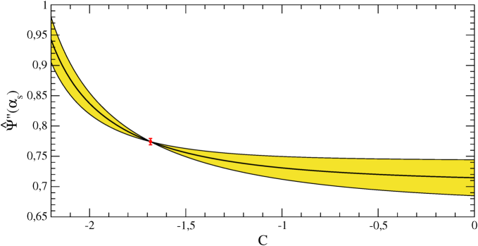
Figure 1: $\widehat{\Psi}^{{}^{\prime\prime}}(\alpha_{s})$ according to eq. (5) as a function of $C$ for $\alpha_{s}(M_{\tau})=0.316$. The yellow band corresponds to either removing or doubling the ${\cal O}(a^{4})$ correction to estimate the respective uncertainty. In the red point, where ${\cal O}(a^{4})$ vanishes, the third order is taken as the error. For further discussion, see the text.

To this end, figure 1 displays a numerical account of the behaviour of $\widehat{\Psi}^{{}^{\prime\prime}}$ as a function of the scheme parameter $C$. As we are interested in applications to hadronic $\tau$ decays in the future, for definiteness, we have chosen $\alpha_{s}(M_{\tau})=0.316$ in the ${\overline{\rm MS}}$ scheme, which corresponds to the current PDG average $\alpha_{s}(M_{Z})=0.1181$ pdg15 . The coupling $\widehat{\alpha}_{s}(Q)$ required in the prefactor has been determined by directly solving eq. (52) numerically, not via the expansion (4). In order to estimate the uncertainty in the perturbative prediction, the fourth order term is either removed or doubled. The steepest curve in figure 1 then corresponds to setting the ${\cal O}(a_{Q}^{4})$ contribution to zero and the flattest one to doubling it. The yellow band hence corresponds to the region of expected values for $\widehat{\Psi}^{{}^{\prime\prime}}$, depending on the parameter $C$.

It is observed that at $C=-1.683$ the ${\cal O}(a_{Q}^{4})$ correction vanishes. Interestingly enough, this value is surprisingly close to $C=-5/3$ in large-$\beta_{0}$, which enters the construction of the invariant coupling (39) in the ${\overline{\rm MS}}$ scheme, though, presumably, this is merely a coincidence. The red data point then indicates an estimate where the uncertainty is taken to be the size of the third-order term. At this value of $C$, the third-order correction has already turned negative and, beyond it, also the ${\cal O}(a_{Q}^{4})$ contribution changes sign. This is an indication that in the respective region of $C$ the contributions from IR and UV renormalons are more balanced. To obtain a more complete picture, also the uncertainty of $\alpha_{s}$ should be folded in. From the PDG average $\alpha_{s}(M_{Z})=0.1181(13)$ pdg15 , we deduce $\alpha_{s}(M_{\tau})=0.316(10)$. Numerically, our result at $C=-1.683$ then reads

$$\widehat{\Psi}^{{}^{\prime\prime}}(C=-1.683)\,=\,0.774\pm 0.005^{\,+\,0.058}_{\,-\,0.052}\,=\,0.774^{\,+\,0.058}_{\,-\,0.052}\,,$$ (59)

where the first error corresponds to the ${\cal O}(a_{Q}^{3})$ correction also displayed in figure 1, while the second error results from the current uncertainty in $\alpha_{s}$. The total error on the right-hand side has been obtained by adding the individual uncertainties in quadrature.

The value (59) can be compared to the result at $C=0$,

$$\widehat{\Psi}^{{}^{\prime\prime}}(C=0)\,=\,0.715\pm 0.030^{\,+\,0.040}_{\,-\,0.038}\,=\,0.715^{\,+\,0.050}_{\,-\,0.048}\,.$$ (60)

The two predictions (59) and (60) are found to be compatible and have similar uncertainties. At present, the error on $\alpha_{s}$ is dominant. While in the prediction (59), the estimated uncertainty from missing higher orders is substantially reduced, its sensitivity to $\alpha_{s}$ and its uncertainty is increased. This is due to the fact that at $C=-1.683$, symmetrising the error, one finds $\widehat{\alpha}_{s}=0.610\pm 0.045$. This increased sensitivity on $\alpha_{s}$ may also be seen as a virtue if one aims at an extraction of $\alpha_{s}$ along the lines of bj08 ; bgjmmop12 ; bgmop14 ; pr16 . In this respect, further understanding of the behaviour of the perturbative series, for example, through models for the Borel transform in the spirit of ref. bj08 , could be helpful. As a last remark it is pointed out that at the scale of $M_{\tau}$, for $C<-2$, the scheme transformation ceases to be perturbative and breaks down. Therefore, such values should be discarded for phenomenology.

We proceed with our second step of also expressing the coupling $a_{Q}$ within the curly brackets of eq. (5) in terms of $\hat{a}_{Q}$. As a matter of principle, we could introduce two different scheme constants $C_{m}$ and $C_{a}$, related to mass and coupling renormalisation, respectively, since the global prefactor originates from the quark mass, and the remaining expansion concerns the QCD coupling. To keep the discussion more transparent, however, we prefer to only use a single common constant $C=C_{m}=C_{a}$. Then the expansion in $\hat{a}_{Q}$ takes the form

$$\widehat{\Psi}^{{}^{\prime\prime}}(\widehat{\alpha}_{s}) = [\widehat{\alpha}_{s}(Q)]^{8/9}\big{\{}\,1+(5.4568+2\,C)\,\hat{a}_{Q}+(25.452+26.747\,C+4.25\,C^{2})\,\hat{a}_{Q}^{2}$$

$$+ (142.44+212.99\,C+94.483\,C^{2}+9.2083\,C^{3})\,\hat{a}_{Q}^{3}$$

$$+ (932.71+1625.0\,C+1099.8\,C^{2}+291.95\,C^{3}+20.143\,C^{4})\,\hat{a}_{Q}^{4}+\ldots\big{\}}.$$ (61)

The corresponding graphical representation of this result is displayed in figure 2. In this case, the order $\hat{a}^{4}$ correction does not vanish for any sensible value of $C$. The smallest uncertainty is assumed around $C\approx-0.9$, at which one deduces

$$\widehat{\Psi}^{{}^{\prime\prime}}(C=-0.9)\,=\,0.753\pm 0.022^{\,+\,0.050}_{\,-\,0.046}\,=\,0.753^{\,+\,0.055}_{\,-\,0.051}\,.$$ (62)

In figure 2, the first error is shown as the red data point and the second again corresponds to the uncertainty induced from the error on $\alpha_{s}$. In view of the large $\alpha_{s}$ error, the result (62) is again fully compatible with (59) and (60).

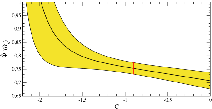
Figure 2: $\widehat{\Psi}^{{}^{\prime\prime}}(\widehat{\alpha}_{s})$ according to eq. (5) as a function of $C$ for $\alpha_{s}(M_{\tau})=0.316$. The yellow band corresponds to either removing or doubling the ${\cal O}(\hat{a}^{4})$ correction to estimate the respective uncertainty. At the red point, the uncertainty resulting from the ${\cal O}(\hat{a}^{4})$ contribution is minimal. For further discussion, see the text.

Let us now turn to the decay of the Higgs boson into quark-antiquark pairs. The corresponding decay width is given by

$$\Gamma(H\to q\bar{q})\,=\,\frac{\sqrt{2}\,G_{F}}{M_{H}}\,\mbox{\rm Im}\Psi\big{(}M_{H}^{2}+i0\big{)}\,\equiv\,\frac{N_{c}\,G_{F}M_{H}}{4\sqrt{2}\pi}\,\widehat{m}_{q}^{2}\,\widehat{R}\big{(}\alpha_{s}(M_{H})\big{)}\,,$$ (63)

which defines the function $\widehat{R}\big{(}\alpha_{s}(M_{H})\big{)}$. We proceed in analogy to the case of $\Psi^{{}^{\prime\prime}}$ by first expressing only the global prefactor in terms of the coupling $\widehat{\alpha}_{s}$, which results in

$$\widehat{R}(\alpha_{s}) = [\widehat{\alpha}_{s}(Q)]^{24/23}\big{\{}\,1+(8.0176+2\,C)\,a_{Q}+(46.732+18.557\,C+0.08333\,C^{2})\,a_{Q}^{2}$$

$$+ (142.12+117.09\,C-1.5384\,C^{2}-0.05093\,C^{3})\,a_{Q}^{3}$$

$$- (544.67-426.17\,C+22.522\,C^{2}-2.2856\,C^{3}-0.04774\,C^{4})\,a_{Q}^{4}+\ldots\big{\}}.$$ (64)

Here the number of flavours $N_{f}=5$ and $Q=M_{H}$. For $\alpha_{s}(M_{H})=0.1127$, a graphical representation of $\widehat{R}(\alpha_{s})$ as a function of $C$ is given in figure 3. Because the coupling now is much smaller than at the $\tau$ scale, the perturbative expansion converges faster, and thus the typical ${\cal O}(a^{4})$ term is substantially smaller than the order $a^{3}$ correction at $C=1.362$, where ${\cal O}(a^{4})$ vanishes. This is obvious from the large error bar of the red point. The corresponding numerical result reads

$$\widehat{R}(C=1.362)\,=\,0.1387\pm 0.0013\pm 0.0020\,=\,0.1387\pm 0.0024\,,$$ (65)

where the second error again results from the variation $\alpha_{s}(M_{H})=0.1127(12)$ which has been deduced from the PDG average. Still, even though the large ${\cal O}(a^{3})$ uncertainty has been assumed, the current error from the $\alpha_{s}$ input is even bigger.

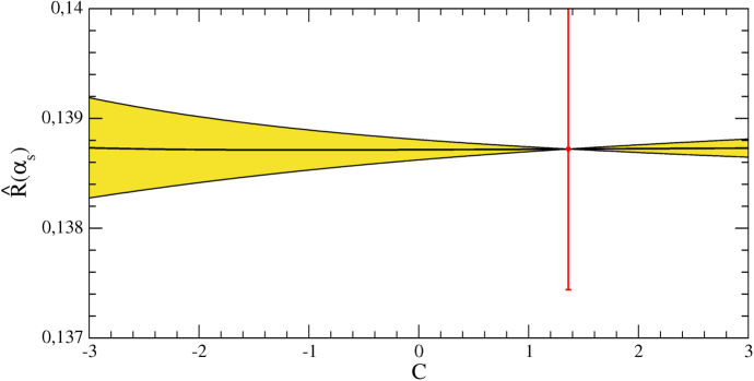
Figure 3: $\widehat{R}(\alpha_{s})$ according to eq. (5) as a function of $C$ for $\alpha_{s}(M_{H})=0.1127$. The yellow band corresponds to either removing or doubling the ${\cal O}(a^{4})$ correction to estimate the respective uncertainty. In the red point, where ${\cal O}(a^{4})$ vanishes, the third order is taken as the error. For further discussion, see the text.

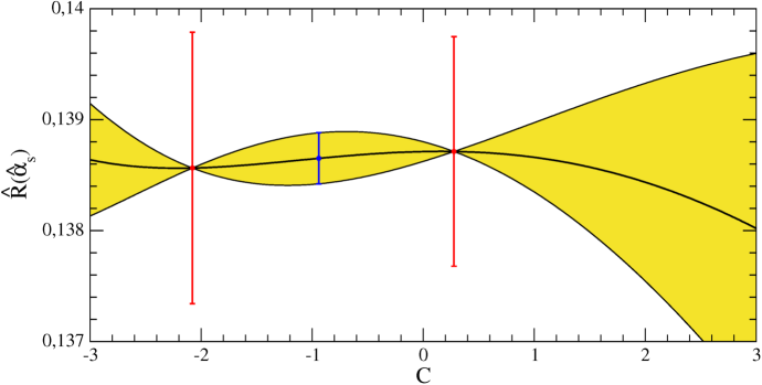
Figure 4: $\widehat{R}(\widehat{\alpha}_{s})$ according to eq. (5) as a function of $C$ for $\alpha_{s}(M_{H})=0.1127$. The yellow band corresponds to either removing or doubling the ${\cal O}(\hat{a}^{4})$ correction to estimate the respective uncertainty. In the red points, where ${\cal O}(\hat{a}^{4})$ vanishes, the third order is taken as the error. For further discussion, see the text.

Like for $\Psi^{{}^{\prime\prime}}$, also for the Higgs decay, as a second step, we express the remaining $\alpha_{s}$ series in powers of $\hat{a}$. This yields

$$\widehat{R}(\widehat{\alpha}_{s}) = [\widehat{\alpha}_{s}(Q)]^{24/23}\big{\{}\,1+(8.0176+2\,C)\,\hat{a}_{Q}+(46.732+33.924\,C+3.9167\,C^{2})\,\hat{a}_{Q}^{2}$$

$$+ (141.19+315.38\,C+103.88\,C^{2}+7.6157\,C^{3})\,\hat{a}_{Q}^{3}$$

$$- (524.03-1491.9\,C-1353.1\,C^{2}-277.97\,C^{3}-14.756\,C^{4})\,\hat{a}_{Q}^{4}+\ldots\big{\}},$$ (66)

and the corresponding behaviour as a function of $C$ is presented in figure 4. This time two values of $C$ are found, at which the ${\cal O}(\hat{a}^{4})$ correction vanishes, and they are again displayed as the red data points. In both cases, like before the corresponding uncertainty inferred from the size of the third order is much larger than a typical fourth order term. The corresponding numerical results are given by

$$\widehat{R}(C=-2.079)\,=\,0.1386\pm 0.0012\pm 0.0020\,=\,0.1386\pm 0.0023\,,$$ (67)

and

$$\widehat{R}(C=0.277)\,=\,0.1387\pm 0.0010\pm 0.0020\,=\,0.1387\pm 0.0022\,,$$ (68)

where the second error once more is due to the $\alpha_{s}$ uncertainty and the final errors result from a quadratic average. In a situation like this, in our opinion a conservative estimate of higher-order corrections can be obtained by assuming the maximal ${\cal O}(\hat{a}^{4})$ correction between those two points and taking that as the perturbative uncertainty. This approach is shown as the blue point, and the numerical value reads

$$\widehat{R}(C=-0.94)\,=\,0.1387\pm 0.0002\pm 0.0020\,=\,0.1387\pm 0.0020\,.$$ (69)

It is clear that now the higher-order uncertainty is completely negligible with respect to the present error in $\alpha_{s}$.

To summarise, rewriting the perturbative expansion in terms of the coupling $\widehat{\alpha}_{s}$ of eq. (52) introduces interesting approaches to improve the convergence of the series for the known low-order corrections, before the asymptotic behaviour sets in. We demonstrated this explicitly for the correlator $\Psi^{{}^{\prime\prime}}(s)$ at the scale $M_{\tau}$ and for the decay of the Higgs boson into quarks which is related to $\mbox{\rm Im}\Psi(s)$ at the scale $M_{H}$. In both examples, however, the parametric uncertainty induced by the error on $\alpha_{s}$ dominates. This is in part due to the recent increase in the $\alpha_{s}$ uncertainty of the PDG average pdg15 by more than a factor of two, in view of an earlier analysis of $\alpha_{s}$ determinations from lattice QCD by the FLAG collaboration flag14 . Hence, we expect our findings to increase in importance when the uncertainty on $\alpha_{s}$ again shrinks in the future. Still, in view of the potential to strengthen the sensitivity on $\alpha_{s}$, our approach could also open promising options for improved non-lattice $\alpha_{s}$ determinations.

6 Conclusions

The scalar correlation function is one of the basic QCD two-point correlators with important phenomenological applications for the decay of the Higgs boson to quark-antiquark pairs djou08 , determinations of light quark masses from QCD sum rules jop02 ; jop06 and contributions to hadronic decays of the $\tau$ lepton pp98 ; pp99 ; gjpps03 . Presently, the perturbative expansion of the scalar correlator is known up to order $\alpha_{s}^{4}$ in the strong coupling bck05 .

Three physical functions related to the scalar correlator play a role for phenomenological studies: $\mbox{\rm Im}\Psi(s)$ in Higgs decay, $\Psi^{{}^{\prime\prime}}(s)$ for quark-mass extractions and $D^{L}(s)$ in finite-energy sum rule analyses of hadronic $\tau$ decays. From the known perturbative coefficients it is observed that the renormalisation-group resummed $D^{L}(s)$ only depends on the independent coefficients $d_{n,1}$, and those corrections turn out much larger than the ones for $\Psi^{{}^{\prime\prime}}(s)$ and $\mbox{\rm Im}\Psi(s)$, for which combinations of the $d_{n,1}$ and $d_{n,k}$ with $k>1$ appear. The latter coefficients are calculable from the renormalisation group and only depend on lower-order $d_{n,1}$, $\beta$-function coefficients, and those of the mass anomalous dimension.

In order to understand this pattern of higher-order corrections better, we reviewed the results for the scalar correlator in the large-$\beta_{0}$ approximation bkm00 , and derived compact expressions for the correlators $\Psi^{{}^{\prime\prime}}(s)$ and $D^{L}(s)$ in terms of Borel transforms, which directly give access to the renormalon structure of the respective correlators. While this structure in the case of $\Psi^{{}^{\prime\prime}}(s)$ is analogous to the one of the Adler function, double and single IR renormalon poles for $u\geq 2$, with only a single pole at $u=2$, as well as double and single UV poles for $u\leq-1$, for the correlator $D^{L}(s)$ an additional single pole at $u=1$ is found. The origin of this spurious pole, which is suspected to be of UV origin, can be traced back to the divergent subtraction $\Psi(0)/s$ that is performed in the construction of $D^{L}(s)$. While the pole at $u=1$ is present in the coefficients $d_{n,1}$, for $\Psi^{{}^{\prime\prime}}(s)$ and $\mbox{\rm Im}\Psi(s)$ it is cancelled by corresponding contributions to the dependent coefficients $d_{n,k}$ with $k>1$.

Another feature of the scalar correlator that becomes apparent from the large-$\beta_{0}$ approximation is the appearance of a regular contribution that is related to the renormalisation of the global mass factor $m^{2}$. By rewriting this prefactor in terms of the renormalisation-group invariant quark mass $\widehat{m}$, one is left with the logarithmic term in eq. (3), which depends on the leading-order RG coefficients $\beta_{1}$ and $\gamma_{m}^{(1)}$, as well as the renormalisation scheme of the coupling in the prefactor. Expressing this prefactor in terms of the coupling $\widehat{\alpha}_{s}$ of eq. (39), which can be considered an invariant coupling in large-$\beta_{0}$, the regular logarithmic contribution is resummed. Improvements in the behaviour of the perturbative series were also discussed in section 3, and it was concluded that this is in part due to shifting the contribution of UV renormalon poles, in particular the lowest-lying one at $u=-1$, to lower orders. Generally, however, it has to be acknowledged that for the scalar correlator the large-$\beta_{0}$ limit does not provide a satisfactory representation of the full QCD case.

In order to mimic as much as possible the large-$\beta_{0}$ case, in section 4, we attempted to define a scheme-invariant coupling also for full QCD. Whereas it appears to be impossible to do this in a universal way, that is, independent of any observable, in eq. (52) we presented the definition of a coupling $\widehat{\alpha}_{s}$ whose running is renormalisation-group invariant in the sense that it only depends on the invariant coefficients $\beta_{1}$ and $\beta_{2}$, and is given by the simple $\beta$-function of eq. (55). The scheme dependence of $\widehat{\alpha}_{s}$ is then parametrised by a single parameter $C$ which corresponds to transformations of the QCD scale parameter $\Lambda$.

Phenomenological applications of re-expressing the perturbative series of $\Psi^{{}^{\prime\prime}}(s)$ at the $\tau$-mass scale, and $\mbox{\rm Im}\Psi(s)$ at $M_{H}$, in terms of $\widehat{\alpha}_{s}$, were investigated in section 5. To this end, we considered two cases: a first, in which only the $\alpha_{s}$-prefactor, originating from the quark mass, is rewritten in $\widehat{\alpha}_{s}$, and the remaining series is kept in the ${\overline{\rm MS}}$ scheme, and a second case, in which the whole series is expressed in terms of the coupling $\widehat{\alpha}_{s}$. Generally, it can be concluded that appropriate choices of $C$ allow for an improvement of the behaviour of the perturbative series for the first few known orders. This is, however, achieved at the expense of an increase in the value of the coupling, either only in the prefactor, or also in the remaining expansion terms, which leads to an increased sensitivity to $\alpha_{s}$ and also its uncertainty.

In an era in which just recently the error on the PDG average of the strong coupling pdg15 has increased by more than a factor of two, in view of an earlier analysis of $\alpha_{s}$ determinations from lattice QCD by the FLAG collaboration flag14 , we find that in all considered cases the uncertainty of our perturbative predictions is dominated by the error on $\alpha_{s}$. Therefore, in the investigated examples, currently, improvements in the perturbative series appear to be a secondary issue. Still, when our knowledge on the value of $\alpha_{s}$ at some point returns to a precision comparable to previous estimates, the uncertainty due to higher-order corrections becomes of a similar size, and optimising the series by appropriate scheme choices through variation of the parameters $C$ should allow for refined perturbative predictions.

On the other hand, the increased sensitivity on $\alpha_{s}$ for certain ranges of $C$ can also be taken as a virtue if one aims at determinations of $\alpha_{s}$, for example from hadronic $\tau$ decay spectra along the lines of refs. bj08 ; bgjmmop12 ; bgmop14 ; pr16 , as this could result in reduced equivalent uncertainties in the ${\overline{\rm MS}}$ coupling. A preliminary assessment of such an approach is performed in ref. bjm16 , for the perturbative expansion of the Adler function and the total $\tau$ hadronic width, before we embark on a full-fledged analysis of the decay spectra. In this respect, also analysing models for the Borel transform in the coupling $\widehat{\alpha}_{s}$, along the lines of ref. bj08 , could provide additional helpful insights.

Since a substantial part of the improvements results from rewriting global prefactors of $\alpha_{s}$, investigating other observables which include such factors and suffer from large perturbative corrections could be rather promising. These factors may either be explicitly present, like for example in gluonium correlation functions which carry a global factor $\alpha_{s}^{2}$, or may emerge from quark-mass factors, similarly to the scalar correlator, as in the case of the total semi-leptonic $B$-meson decay rate which is proportional to $m_{b}^{5}$. It is to be expected that also in these applications the perturbative expansion could be improvable by adequate scheme choices for the coupling $\widehat{\alpha}_{s}$.

Appendix A Renormalisation group functions and dependent coefficients

In our notation, the QCD $\beta$-function and mass anomalous dimension are defined as:

$$-\,\mu\,\frac{{\rm d}a}{{\rm d}\mu} \equiv \beta(a)\,=\,\beta_{1}\,a^{2}+\beta_{2}\,a^{3}+\beta_{3}\,a^{4}+\beta_{4}\,a^{5}+\ldots\,,$$ (70)

$$\vbox{\vskip 17.07164pt}-\,\frac{\mu}{m}\,\frac{{\rm d}m}{{\rm d}\mu} \equiv \gamma_{m}(a)\,=\,\gamma_{m}^{(1)}\,a+\gamma_{m}^{(2)}\,a^{2}+\gamma_{m}^{(3)}\,a^{3}+\gamma_{m}^{(4)}\,a^{4}+\ldots\,.$$ (71)

It is assumed that we work in a mass-independent renormalisation scheme and in this study throughout the modified minimal subtraction scheme ${\overline{\rm MS}}$ is used. To make the presentation self-contained, below the known coefficients of the $\beta$-function and mass anomalous dimension in the given conventions shall be provided. Numerically, for $N_{c}=3$ the first four coefficients of the $\beta$-function are given by tvz80 ; lrv97 ; cza04 ; bck16

$$\beta_{1} = \mbox{$\frac{11}{2}$}-\mbox{$\frac{1}{3}$}\,N_{f}\,,\qquad\beta_{2}\,=\,\mbox{$\frac{51}{4}$}-\mbox{$\frac{19}{12}$}\,N_{f}\,,\qquad\beta_{3}\,=\,\mbox{$\frac{2857}{64}$}-\mbox{$\frac{5033}{576}$}\,N_{f}+\mbox{$\frac{325}{1728}$}\,N_{f}^{2}\,,$$

$$\vbox{\vskip 17.07164pt}\beta_{4} = \mbox{$\frac{149753}{768}$}+\mbox{$\frac{891}{32}$}\,\zeta_{3}-\left(\mbox{$\frac{1078361}{20736}$}+\mbox{$\frac{1627}{864}$}\,\zeta_{3}\right)N_{f}+\left(\mbox{$\frac{50065}{20736}$}+\mbox{$\frac{809}{1296}$}\,\zeta_{3}\right)N_{f}^{2}+\mbox{$\frac{1093}{93312}$}\,N_{f}^{3}\,,$$

$$\vbox{\vskip 17.07164pt}\beta_{5} = \mbox{$\frac{8157455}{8192}$}+\mbox{$\frac{621885}{1024}$}\,\zeta_{3}-\mbox{$\frac{88209}{1024}$}\,\zeta_{4}-\mbox{$\frac{144045}{256}$}\,\zeta_{5}$$

$$- \left(\mbox{$\frac{336460813}{995328}$}+\mbox{$\frac{1202791}{10368}$}\,\zeta_{3}-\mbox{$\frac{33935}{3072}$}\,\zeta_{4}-\mbox{$\frac{1358995}{13824}$}\,\zeta_{5}\right)N_{f}$$

$$+ \left(\mbox{$\frac{25960913}{995328}$}+\mbox{$\frac{698531}{41472}$}\,\zeta_{3}-\mbox{$\frac{5263}{2304}$}\,\zeta_{4}-\mbox{$\frac{5965}{648}$}\,\zeta_{5}\right)N_{f}^{2}$$

$$- \left(\mbox{$\frac{630559}{2985984}$}+\mbox{$\frac{24361}{62208}$}\,\zeta_{3}-\mbox{$\frac{809}{6912}$}\,\zeta_{4}-\mbox{$\frac{115}{1152}$}\,\zeta_{5}\right)N_{f}^{3}+\left(\mbox{$\frac{1205}{1492992}$}-\mbox{$\frac{19}{5184}$}\,\zeta_{3}\right)\,N_{f}^{4}\,,$$ (72)

and the first five for $\gamma_{m}(a)$ are found to be vlr97 ; bck14

$$\gamma_{m}^{(1)} = 2\,,\qquad\gamma_{m}^{(2)}\,=\,\mbox{$\frac{101}{12}$}-\mbox{$\frac{5}{18}$}\,N_{f}\,,\qquad\gamma_{m}^{(3)}\,=\,\mbox{$\frac{1249}{32}$}-\left(\mbox{$\frac{277}{108}$}+\mbox{$\frac{5}{3}$}\,\zeta_{3}\right)N_{f}-\mbox{$\frac{35}{648}$}\,N_{f}^{2}\,,$$

$$\vbox{\vskip 17.07164pt}\gamma_{m}^{(4)} = \mbox{$\frac{4603055}{20736}$}+\mbox{$\frac{1060}{27}$}\,\zeta_{3}-\mbox{$\frac{275}{4}$}\,\zeta_{5}-\left(\mbox{$\frac{91723}{3456}$}+\mbox{$\frac{2137}{72}$}\,\zeta_{3}-\mbox{$\frac{55}{8}$}\,\zeta_{4}-\mbox{$\frac{575}{36}$}\,\zeta_{5}\right)N_{f}$$

$$+ \left(\mbox{$\frac{2621}{15552}$}+\mbox{$\frac{25}{36}$}\,\zeta_{3}-\mbox{$\frac{5}{12}$}\,\zeta_{4}\right)N_{f}^{2}-\left(\mbox{$\frac{83}{7776}$}-\mbox{$\frac{1}{54}$}\,\zeta_{3}\right)N_{f}^{3}\,.$$

$$\vbox{\vskip 17.07164pt}\gamma_{m}^{(5)} = \mbox{$\frac{99512327}{82944}$}+\mbox{$\frac{23201233}{62208}$}\,\zeta_{3}+\mbox{$\frac{3025}{16}$}\,\zeta_{3}^{2}-\mbox{$\frac{349063}{2304}$}\,\zeta_{4}-\mbox{$\frac{28969645}{15552}$}\,\zeta_{5}+\mbox{$\frac{15125}{32}$}\,\zeta_{6}+\mbox{$\frac{25795}{32}$}\,\zeta_{7}$$

$$- \left(\mbox{$\frac{150736283}{746496}$}+\mbox{$\frac{391813}{1296}$}\,\zeta_{3}+\mbox{$\frac{2365}{144}$}\,\zeta_{3}^{2}-\mbox{$\frac{1019371}{6912}$}\,\zeta_{4}-\mbox{$\frac{12469045}{31104}$}\,\zeta_{5}+\mbox{$\frac{39875}{288}$}\,\zeta_{6}+\mbox{$\frac{56875}{432}$}\,\zeta_{7}\right)N_{f}$$

$$+ \left(\mbox{$\frac{660371}{186624}$}+\mbox{$\frac{251353}{15552}$}\,\zeta_{3}+\mbox{$\frac{725}{216}$}\,\zeta_{3}^{2}-\mbox{$\frac{41575}{3456}$}\,\zeta_{4}-\mbox{$\frac{33005}{5184}$}\,\zeta_{5}+\mbox{$\frac{2875}{432}$}\,\zeta_{6}\right)N_{f}^{2}$$

$$+ \left(\mbox{$\frac{91865}{746496}$}+\mbox{$\frac{803}{2592}$}\,\zeta_{3}+\mbox{$\frac{7}{72}$}\,\zeta_{4}-\mbox{$\frac{10}{27}$}\,\zeta_{5}\right)N_{f}^{3}-\left(\mbox{$\frac{65}{31104}$}+\mbox{$\frac{5}{1944}$}\,\zeta_{3}-\mbox{$\frac{1}{216}$}\,\zeta_{4}\right)N_{f}^{4}\,.$$ (73)

The dependent perturbative coefficients $d_{n,k}$ with $k>1$ can be expressed in terms of the independent coefficients $d_{n,1}$, and coefficients of the QCD $\beta$-function and mass anomalous dimension. In particular, the coefficients $d_{n,2}$, which are required in eq. (10), take the form

$$d_{n,2}\,=\,-\,\frac{1}{2}\,\gamma_{m}^{(n)}d_{0,1}-\frac{1}{4}\sum\limits_{k=1}^{n-1}\big{(}2\gamma_{m}^{(n-k)}+k\,\beta_{n-k}\big{)}d_{k,1}\,.$$ (74)

Explicitly, at $N_{c}=3$ and up to the fourth order, they read:

$$d_{1,2} = -\,1\,,\qquad d_{2,2}\,=\,-\,\mbox{$\frac{53}{3}$}+\mbox{$\frac{11}{18}$}\,N_{f}\,,$$

$$\vbox{\vskip 17.07164pt}d_{3,2} = -\,\mbox{$\frac{49349}{144}$}+\mbox{$\frac{585}{8}$}\zeta_{3}+\left(\mbox{$\frac{11651}{432}$}-\mbox{$\frac{59}{12}$}\zeta_{3}\right)N_{f}-\left(\mbox{$\frac{275}{648}$}-\mbox{$\frac{1}{9}$}\zeta_{3}\right)N_{f}^{2}\,,$$

$$\vbox{\vskip 17.07164pt}d_{4,2} = -\,\mbox{$\frac{49573615}{6912}$}+\mbox{$\frac{535759}{192}$}\zeta_{3}-\mbox{$\frac{30115}{96}$}\zeta_{5}+\left(\mbox{$\frac{56935973}{62208}$}-\mbox{$\frac{243511}{864}$}\zeta_{3}+\mbox{$\frac{5}{6}$}\zeta_{4}+\mbox{$\frac{1115}{48}$}\zeta_{5}\right)N_{f}$$ (75)

$$-\,\left(\mbox{$\frac{6209245}{186624}$}-\mbox{$\frac{250}{27}$}\zeta_{3}+\mbox{$\frac{25}{36}$}\zeta_{5}\right)N_{f}^{2}+\left(\mbox{$\frac{985}{2916}$}-\mbox{$\frac{5}{54}$}\zeta_{3}\right)N_{f}^{3}\,.$$

Appendix B The coefficients ${\cal D}_{n}^{(1)}$ and $H_{n}^{(1)}$

Here, we provide the coefficients ${\cal D}_{n}^{(1)}$ and $H_{n}^{(1)}$, required to predict the perturbative coefficients $d_{n,1}$ in the large-$\beta_{0}$ approximation up to fifth order.

$${\cal D}_{1}^{(1)} = -\,1\,,\quad{\cal D}_{2}^{(1)}\,=\,-\,\mbox{$\frac{22}{3}$}\,,\quad{\cal D}_{3}^{(1)}\,=\,-\,\mbox{$\frac{275}{6}$}+12\,\zeta_{3}\,,\quad{\cal D}_{4}^{(1)}\,=\,-\,\mbox{$\frac{7880}{27}$}+80\,\zeta_{3}\,,$$

$$\vbox{\vskip 17.07164pt}{\cal D}_{5}^{(1)} = -\,\mbox{$\frac{324385}{162}$}+\mbox{$\frac{1000}{3}$}\,\zeta_{3}+600\,\zeta_{5}\,,\quad{\cal D}_{6}^{(1)}\,=\,-\,\mbox{$\frac{1224355}{81}$}+\mbox{$\frac{10000}{9}$}\,\zeta_{3}+6000\,\zeta_{5}\,.$$ (76)

$$H_{2}^{(1)} = \mbox{$\frac{51}{2}$}\,,\quad H_{3}^{(1)}\,=\,-\,\mbox{$\frac{585}{8}$}+18\,\zeta_{3}\,,\quad H_{4}^{(1)}\,=\,\mbox{$\frac{15511}{72}$}-54\,\zeta_{3}\,,$$

$$\vbox{\vskip 17.07164pt}H_{5}^{(1)} = -\,\mbox{$\frac{520771}{576}$}+\mbox{$\frac{585}{4}$}\,\zeta_{3}+\mbox{$\frac{27}{4}$}\,\zeta_{4}+270\,\zeta_{5}\,,$$

$$\vbox{\vskip 17.07164pt}H_{6}^{(1)} = \mbox{$\frac{19577503}{4320}$}-\mbox{$\frac{2021}{6}$}\,\zeta_{3}-\mbox{$\frac{9}{2}$}\,\zeta_{4}-\mbox{$\frac{8946}{5}$}\,\zeta_{5}\,.$$ (77)

Appendix C The subtraction constant $\Psi(0)$

In order to understand the structure of the subtraction constant $\Psi(0)$, examining the lowest perturbative order is sufficient. For definiteness, we consider the case of the current (2) that plays a role in hadronic $\tau$ decays. $\Psi(0)$ receives contributions from the normal-ordered quark condensate and a perturbative term proportional to $m^{4}$. At lowest order it reads:

$$\Psi(0) = -\,(m_{u}-m_{s})\big{[}\,\langle\Omega|\!:\!\bar{u}u\!:\!|\Omega\rangle-\langle\Omega|\!:\!\bar{s}s\!:\!|\Omega\rangle\,\big{]}$$

$$+\,4iN_{c}\,(m_{u}-m_{s})\big{[}\,m_{u}I_{m_{u}}-m_{s}I_{m_{s}}\,\big{]}\,,$$ (78)

where $I_{m}$ is the UV divergent massive scalar vacuum-bubble integral

$$I_{m}\,\equiv\,\mu^{2\varepsilon}\!\!\int\!\frac{{\rm d}^{D}\!k}{(2\pi)^{D}}\,\frac{1}{(k^{2}-m^{2}+i0)}\,=\,\frac{i}{(4\pi)^{2}}\,m^{2}\,\biggl{\{}\,\frac{1}{\hat{\varepsilon}}-\ln\frac{m^{2}}{\mu^{2}}+1+{\cal O}(\varepsilon)\,\biggr{\}}\,.$$ (79)

The explicit expression for $I_{m}$ has been provided in dimensional regularisation with $D=4-2\varepsilon$ and $1/\hat{\varepsilon}\equiv 1/\varepsilon-\gamma_{E}+\ln(4\pi)$, but the particular regularisation scheme is inessential for our argument.

Precisely the same massive scalar vacuum-bubble contribution as in the second line of eq. (C) also arises when rewriting the normal-ordered condensates in terms of non-normal-ordered minimally subtracted quark condensates sc88 ; jm93 . Therefore, $\Psi(0)$ can also be expressed as

$$\Psi(0)\,=\,-\,(m_{u}-m_{s})\big{[}\,\langle\Omega|\bar{u}u|\Omega\rangle-\langle\Omega|\bar{s}s|\Omega\rangle\,\big{]}\,,$$ (80)

which absorbs the mass logarithms in the definition of the quark condensate. Due to a Ward identity, the condensate contribution in $\Psi(0)$ does not receive higher-order corrections, and at least at next-to-leading order, it has been checked that the perturbative term matches the vacuum-bubble structure that arises when rewriting $\langle\Omega|\!:\!\bar{q}q\!:\!|\Omega\rangle$ in terms of $\langle\Omega|\bar{q}q|\Omega\rangle$ gen90 . It is expected that this behaviour, and hence also the form of eq. (80), should remain the same to all orders. As an aside, it may be remarked that for the pseudoscalar channel the combination (80) with flavour sums of quark masses as well as condensates is precisely what appears in the Gell-Mann-Oakes-Renner relation gmor68 ; mj02 .

As we have seen, the subtraction constant $\Psi(0)$ suffers from a UV divergence originating from the perturbative quark-mass correction in eq. (C). Even though this contribution can be absorbed in the definition of the quark condensate by rewriting normal-ordered in terms of non-normal-ordered condensates, because of the subtraction of $\Psi(0)/s$, the UV divergence reflects itself in the spurious renormalon at $u=1$ in the correlation function $D^{L}(Q^{2})$ of eq. (3).

References

- (1) P.A. Baikov, K.G. Chetyrkin, and J.H. Kühn, Scalar correlator at , Higgs decay into -quarks and bounds on the light quark masses, Phys. Rev. Lett. 96 (2006) 012003, [hep-ph/0511063].
- (2) K.G. Chetyrkin, Correlator of the quark scalar currents and at in pQCD, Phys. Lett. B 390 (1997) 309, [hep-ph/9608318].
- (3) S.G. Gorishnii, A.L. Kataev, S.A. Larin, and L.R. Surguladze, Corrected three loop QCD correction to the correlator of the quark scalar currents and , Mod. Phys. Lett. A 5 (1990) 2703.
- (4) A. Djouadi, The Anatomy of electro-weak symmetry breaking. I: The Higgs boson in the Standard Model, Phys. Rept. 457 (2008) 1–216, [hep-ph/0503172].
- (5) M. Jamin, J.A. Oller and A. Pich, Scalar form factor and light quark masses, Phys. Rev. D 74 (2006) 074009, [hep-ph/0605095].
- (6) M. Jamin, J.A. Oller and A. Pich, Light quark masses from scalar sum rules, Eur. Phys. J. C 24 (2002) 237, [hep-ph/0110194].
- (7) A. Pich and J. Prades, Perturbative quark mass corrections to the tau hadronic width, JHEP 9806 (1998) 013, [hep-ph/9804462].
- (8) A. Pich and J. Prades, Strange quark mass determination from Cabibbo suppressed tau decays, JHEP 9910 (1999) 004, [hep-ph/9909244].
- (9) E. Gámiz, M. Jamin, A. Pich, J. Prades, and F. Schwab, Determination of and from hadronic decays, JHEP 01 (2003) 060, [hep-ph/0212230].
- (10) D.J. Broadhurst, A.L. Kataev, and C.J. Maxwell, Renormalons and multiloop estimates in scalar correlators, Higgs decay and quark-mass sum rule, Nucl. Phys. B 592 (2001) 247, [hep-ph/0007152].
- (11) M. Beneke, Large-order perturbation theory for a physical quantity, Nucl. Phys. B 405 (1993) 424.
- (12) D.J. Broadhurst, Large- expansion of QED: Asymptotic photon propagator and contributions to the muon anomaly, for any number of loops, Z. Phys. C 58 (1993) 339.
- (13) M. Beneke and V.M. Braun, Naive non-Abelianization and resummation of fermion bubble chains, Phys. Lett. B 348 (1995) 513, [hep-ph/9411229].
- (14) M. Beneke, Renormalons, Phys. Rept. 317 (1999) 1–142, [hep-ph/9807443].
- (15) W.A. Bardeen, A.J. Buras, D.W. Duke and T. Muta, Deep inelastic scattering beyond the leading order in asymptotically free gauge theories, Phys. Rev. D 18 (1978) 3998.
- (16) M. Beneke and M. Jamin, and the hadronic width: fixed-order, contour-improved and higher-order perturbation theory, JHEP 0809 (2008) 044, [arXiv:0806.3156 [hep-ph]].
- (17) J.A. Gracey, Quark, gluon and ghost anomalous dimensions at in quantum chromodynamics, Phys. Lett. B 318 (1993) 177, [hep-th/9310063].
- (18) W. Celmaster and R.J. Gonsalves, Renormalization-prescription dependence of the QCD coupling constant, Phys. Rev. D 20 (1979) 1420.
- (19) L.S. Brown, L.G. Yaffe and C.X. Zhai, Large-order perturbation theory for the electromagnetic current current correlation function, Phys. Rev. D 46 (1992) 4712, [hep-ph/9205213].
- (20) M. Beneke, Die Struktur der Störungsreihe in hohen Ordnungen, PhD Thesis, Munich, 1993.
- (21) G. ’t Hooft, Can we make sense out of Quantum Chromodynamics?, Subnucl. Ser. 15 (1979) 943.
- (22) G. Grunberg, Renormalization group improved perturbative QCD, Phys. Lett. B 95 (1980) 70.
- (23) G. Grunberg, Renormalization scheme independent QCD and QED: The method of effective charges, Phys. Rev. D 29 (1984) 2315.
- (24) K.A. Olive et al. (Particle Data Group Collaboration), Review of Particle Physics, Chin. Phys. C 38 (2014) 090001.
- (25) D. Boito, M. Golterman, M. Jamin, A. Mahdavi, K. Maltman, J. Osborne and S. Peris, An updated determination of from decays, Phys. Rev. D 85 (2012) 093015, [arXiv:1203.3146 [hep-ph]].
- (26) D. Boito, M. Golterman, K. Maltman, J. Osborne and S. Peris, Strong coupling from the revised ALEPH data for hadronic decays, Phys. Rev. D 91 (2015) 034003, [arXiv:1410.3528 [hep-ph]].
- (27) A. Pich and A. Rodríguez-Sánchez, Determination of the QCD coupling from ALEPH decay data, [arXiv:1605.06830 [hep-ph]].
- (28) S. Aoki et al., Review of lattice results concerning low-energy particle physics, Eur. Phys. J. C 74 (2014) 2890, [arXiv:1310.8555 [hep-lat]].
- (29) D. Boito, M. Jamin and R. Miravitllas, Scheme variations of the QCD coupling and hadronic decays, Phys. Rev. Lett. 117 (2016) 152001, [arXiv:1606.06175 [hep-ph]].
- (30) O.V. Tarasov, A.A. Vladimirov, and Yu.A. Zharkov, The Gell-Mann-Low function of QCD in the three-loop approximation, Phys. Lett. B, 93 (1980) 429.
- (31) T. van Ritbergen, J.A.M. Vermaseren, and S.A. Larin, The four-loop -function in quantum chromodynamics, Phys. Lett. B, 400 (1997) 379, [hep-ph/9701390].
- (32) M. Czakon, The four-loop QCD -function and anomalous dimensions, Nucl. Phys. B, 710 (2005) 485, [hep-ph/0411261].
- (33) P.A. Baikov, K.G. Chetyrkin and J.H. Kühn, Five-loop running of the QCD coupling constant, [arXiv:1606.08659 [hep-ph]].
- (34) J.A.M. Vermaseren, and S.A. Larin, and T. van Ritbergen, The four-loop quark mass anomalous dimension and the invariant quark mass, Phys. Lett. B, 405 (1997) 327, [hep-ph/9703284].
- (35) P.A. Baikov, K.G. Chetyrkin and J.H. Kühn, Quark mass and field anomalous dimensions to , JHEP 1410 (2014) 76, [arXiv:1402.6611 [hep-ph]].
- (36) V.P. Spiridonov and K.G. Chetyrkin, Nonleading mass corrections and renormalization of the operators and , Sov. J. Nucl. Phys. 47 (1988) 522, [Yad. Fiz. 47 (1988) 818].
- (37) M. Jamin and M. Münz, Current correlators to all orders in the quark masses, Z. Phys. C 60 (1993) 569, [hep-ph/9208201].
- (38) S.C. Generalis, QCD sum rules. 1: Perturbative results for current correlators, J. Phys. G 16 (1990) 785.
- (39) M. Gell-Mann, R.J. Oakes and B. Renner, Behaviour of current divergences under SU(3)SU(3), Phys. Rev. 175 (1968) 2195.
- (40) M. Jamin, Flavour symmetry breaking of the quark condensate and chiral corrections to the Gell-Mann-Oakes-Renner relation, Phys. Lett. B 538 (2002) 71, [hep-ph/0201174].