A decoupled scheme based on the Hermite expansion
to construct lattice Boltzmann models for the compressible
Navier-Stokes equations with arbitrary specific heat ratio

Abstract

A decoupled scheme based on the Hermite expansion to construct lattice Boltzmann models for the compressible Navier-Stokes equations with arbitrary specific heat ratio is proposed. The local equilibrium distribution function including the rotational velocity of particle is decoupled into two parts, i.e. the local equilibrium distribution function of the translational velocity of particle and that of the rotational velocity of particle. From these two local equilibrium functions, two lattice Boltzmann models are derived via the Hermite expansion, namely one is in relation to the translational velocity and the other is connected with the rotational velocity. Accordingly, the distribution function is also decoupled. After this, the evolution equation is decoupled into the evolution equation of the translational velocity and that of the rotational velocity. The two evolution equations evolve separately. The lattice Boltzmann models used in the scheme proposed by this work are constructed via the Hermite expansion, so it is easy to construct new schemes of higher-order accuracy. To validate the proposed scheme, a one dimensional shock tube simulation is performed. The numerical results agree with the analytical solutions very well.

PACS numbers

47.11.-j, 47.10.-g, 47.40.-x

I Introduction

The lattice Boltzmann method(LBM) has been successfully applied to isothermal fluidsChen et al. (1992); Chen and Doolen (1998). However, when it is applied to thermal fluids, the LBM encounters some difficulties. One of them is that the specific heat ratio $\gamma$ in the macroscopic equations derived from the Bhatnager-Gross-Krook(BGK) equation via the Chapman-Enskog expansion is fixed, in other words, the specific heat ratio $\gamma$ is not realistic. Several lattice Boltzmann(LB) schemes with flexible specific heat ratio have been proposedShi et al. (2001); Kataoka and Tsutahara (2004); Watari (2007); Tsutahara et al. (2008). These LB schemes are derived in a similar way. The discrete velocities and the local equilibrium distribution function are determined by a set of constraints which makes sure the macroscopic equations match the thermohydrodynamic equations with certain accuracy. Since 2006, a new way to construct LB models has been developedPhilippi et al. (2006, 2015); Shan et al. (2006); Mattila et al. (2014); Shim (2013a, b); Ansumali et al. (2003); Chikatamarla and Karlin (2006, 2009); Yudistiawan et al. (2010). Contrary to the previous way, the new way derives the discrete velocities and the equilibrium distribution function via the Hermite quadrature and the Hermite expansion. The LB models constructed by the new way are more stable than the LB models constructed by the previous way and it is easy to construct LB models of higher order. In this work, we apply the new way to constructing LB schemes for the compressible Navier-Stokes equations with flexible specific heat ratio. The local equilibrium distribution function including the rotational velocity of particle is decoupled into two parts — one is in relation to the translational velocity and the other is connected with the rotational velocity. The distribution function is also decoupled into two parts accordingly. Two LB models are derived via the Hermite expansion. One is for the distribution function of the translational velocity and the other is for that of the rotational velocity. After this, we decouple the evolution equation into the evolution equation of the translational velocity and that of the rotational velocity. The two evolution equations evolve separately. The decoupled scheme given above is validated by a shock tube simulation. The results of simulation agree with the analytical solutions very well.

II Decoupling the local equilibrium distribution function including the rotational velocity of particle

We begin with the local equilibrium distribution function. The origin that the specific heat ratio is fixed is that gases are supposed to be monatomic, so there is only the translational free degree and the rotational free degree is limited. To describe diatomic gases or polyatomic gases, the rotational velocity of particle should be introduced. The local equilibrium distribution function including the rotational velocity of particle isWatari (2007); Xu et al. (2014)

$$f^{eq}(\bm{\xi},\eta)= \rho\frac{1}{(2\pi R_{g}T)^{\frac{D}{2}}}\frac{1}{(2n\pi R_{g}T)^{\frac{1}{2}}}$$

$$\times\exp{\Big{[}-\frac{(\bm{\xi}-\bm{u})^{2}}{2R_{g}T}-\frac{\eta^{2}}{2nR_{g}T}\Big{]}},$$ (1)

where $\rho$ is the density, $T$ is the absolute temperature, $\bm{u}$ is the macroscopic velocity, $\bm{\xi}$ is the translational velocity of particle, $\eta$ is the rotational velocity of particle, $n$ is the free degree of the rotational velocity of particle, $D$ is the dimension and $R_{g}$ is the universal gas constant.

The dimensionless local equilibrium distribution function is

$$\tilde{f}^{eq}(\tilde{\bm{\xi}},\tilde{\eta})=\frac{\tilde{\rho}}{(2\pi\tilde{\theta})^{\frac{D}{2}}}\frac{1}{(2\pi\tilde{\theta})^{\frac{1}{2}}}\exp\Big{(}-\frac{|\tilde{\bm{\xi}}-\tilde{\bm{u}}|^{2}}{2\tilde{\theta}}\Big{)}\exp\Big{(}-\frac{\tilde{\eta}^{2}}{2\tilde{\theta}}\Big{)},$$ (2)

where $\tilde{f}^{eq}\!=\!f^{eq}\theta_{0}^{N/2}(n\theta_{0})^{1/2}$, $\theta\!=\!R_{g}T$, $\tilde{\rho}\!=\!\rho/\rho_{0}$, $\tilde{\bm{\xi}}\!=\!\bm{\xi}/\sqrt{\theta_{0}}$, $\tilde{\eta}\!=\!\eta/n\sqrt{\theta_{0}}$, $\tilde{\bm{u}}\!=\!\bm{u}/\sqrt{\theta_{0}}$, $\tilde{\theta}\!=\!\tilde{T}=\theta/\theta_{0}$,and $\theta_{0}=R_{g}T_{0}$.

Omitting the tildes on $\rho$, $\bm{\xi}$, $\eta$, $\bm{u}$, $\theta(T)$, we simplify Formula (2)

$$f^{eq}(\bm{\xi},\eta)=\frac{\rho}{(2\pi\theta)^{\frac{D}{2}}}\frac{1}{(2\pi\theta)^{\frac{1}{2}}}\exp\Big{(}-\frac{|{\bm{\xi}}-\bm{u}|^{2}}{2\theta}\Big{)}\exp\Big{(}-\frac{\eta^{2}}{2\theta}\Big{)}.$$ (3)

The dimensionless local equilibrium distribution function can be decoupled into the local equilibrium distribution function of $\bm{\xi}$ and that of $\eta$

$$f^{eq}(\bm{\xi},\eta)=g^{eq}(\bm{\xi})h^{eq}(\eta),$$ (4)

where

$$g^{eq}(\bm{\xi})=\frac{\rho}{(2\pi\theta)^{\frac{D}{2}}}\exp\Big{(}-\frac{|{\bm{\xi}}-\bm{u}|^{2}}{2\theta}\Big{)},$$

$$h^{eq}(\eta)=\frac{1}{(2\pi\theta)^{\frac{1}{2}}}\exp\Big{(}-\frac{\eta^{2}}{2\theta}\Big{)}.$$

Taking the moment integrals of $f^{eq}(\bm{\xi})$, we obtain

$$\rho= \int g^{eq}(\bm{\xi})d\bm{\xi}$$ (5a)

$$\rho\bm{u}= \int g^{eq}(\bm{\xi})\bm{\xi}d\bm{\xi}$$ (5b)

$$\rho(e_{t}+\frac{1}{2}u^{2})= \int g^{eq}(\bm{\xi})\frac{1}{2}\xi^{2}d\bm{\xi}$$ (5c)

where $e_{t}=\displaystyle\frac{D}{2}T$ is the translational internal energy.

Taking the moment integrals of $f^{eq}(\eta)$, we get

$$1= \int h^{eq}(\eta)d\eta$$ (6a)

$$e_{r}= \int h^{eq}(\eta)\frac{n}{2}\eta^{2}d\eta$$ (6b)

where $e_{r}=\displaystyle\frac{n}{2}T=\displaystyle\frac{n}{D}e_{t}$ is the rotational internal energy.

Taking the moment integrals of the local equilibrium distribution function$f^{eq}(\bm{\xi},\eta)$, we obtain

$$\rho= \int\!\!\!\int f^{eq}(\bm{\xi},\eta)d\bm{\xi}d\eta$$ (7a)

$$\rho\bm{u}= \int\!\!\!\int f^{eq}(\bm{\xi},\eta)\bm{\xi}d\bm{\xi}d\eta$$ (7b)

$$\rho(E+\frac{1}{2}u^{2})= \int\!\!\!\int f^{eq}(\bm{\xi},\eta)(\frac{1}{2}\xi^{2}+\frac{n}{2}\eta^{2})d\bm{\xi}d\eta$$ (7c)

where $E=\displaystyle\frac{D+n}{2}T=\displaystyle\frac{D+n}{D}e_{t}$ is the internal energy. It is the sum of the translational energy $e_{t}$ and the rotational energy $e_{r}$.

According to the kinetic theory, we get

$$\rho= \int\!\!\!\int f(\bm{\xi},\eta)d\bm{\xi}d\eta$$ (8a)

$$\rho\bm{u}= \int\!\!\!\int f(\bm{\xi},\eta)\bm{\xi}d\bm{\xi}d\eta$$ (8b)

$$\rho(E+\frac{1}{2}u^{2})= \int\!\!\!\int f(\bm{\xi},\eta)(\frac{1}{2}\xi^{2}+\frac{n}{2}\eta^{2})d\bm{\xi}d\eta$$ (8c)

Now we assume the translational velocity of particle $\bm{\xi}$ is independent of the rotational velocity of particle, so the distribution function $f(\bm{\xi},\eta)$ can be decoupled into $g(\bm{\xi})$ and $h(\eta)$

$$f(\bm{\xi},\eta)=g(\bm{\xi})h(\eta),$$ (9)

where we define

$$f(\bm{\xi},\eta)=\rho b(\bm{\xi}, \eta)=\rho b_{1}(\bm{\xi})h(\eta),$$ (10a)

$$g(\bm{\xi})= \int f(\bm{\xi},\eta)d\eta,$$ (10b)

$$h(\eta)= \int b(\bm{\xi},\eta)d\bm{\xi}.$$ (10c)

Section(III) and Appendix will discuss the reasonableness of this assumption.

It should be noticed that $b(\bm{\xi},\eta)$ is a joint probability distribution, $b_{1}(\bm{\xi})$ and $h(\eta)$ are marginal probability distributions, $g(\bm{\xi})$ is the product of $\rho$ and a marginal probability distribution.

According to Formula(8) and (10), the moments of the distribution function $g(\bm{\xi})$ are

$$\int g(\bm{\xi})d\bm{\xi}= \int\!\!\!\int f(\bm{\xi},\eta)d\bm{\xi}d\eta=\rho,$$ (11a)

$$\int g(\bm{\xi})\bm{\xi}d\bm{\xi}= \int\!\!\!\int f(\bm{\xi},\eta)\bm{\xi}d\bm{\xi}d\eta=\rho\bm{u},$$ (11b)

$$\int g(\bm{\xi})\frac{1}{2}\xi^{2}d\bm{\xi}= \int\!\!\!\int f(\bm{\xi},\eta)\frac{1}{2}\xi^{2}d\bm{\xi}d\eta=\rho(e_{t}+\frac{1}{2}u^{2}).$$ (11c)

Similar to Formula(11), the moments of the distribution function $h(\eta)$ are

$$\int h(\eta)d\eta= \int\!\!\!\int b(\bm{\xi},\eta)d\bm{\xi}d\eta=1$$ (12a)

$$\int h(\eta)\frac{n}{2}\eta^{2}d\eta= \int\!\!\!\int b(\bm{\xi},\eta)\frac{n}{2}\eta^{2}d\bm{\xi}d\eta=e_{r}$$ (12b)

III Decoupling the evolution equation

We have decoupled the equilibrium distribution function $f^{eq}(\bm{\xi},\eta)$ and the distribution function $f(\bm{\xi},\eta)$ in Section II

$$f^{eq}(\bm{\xi},\eta)= g^{eq}(\bm{\xi})h^{eq}(\eta),$$

$$f(\bm{\xi},\eta)= g(\bm{\xi})h(\eta).$$

After decoupling $f^{eq}(\bm{\xi},\eta)$ and $f(\bm{\xi},\eta)$, we can decouple the evolution equation of $f(\bm{\xi},\eta)$. The evolution equation of $f(\bm{\xi},\eta)$ can be expressed as

$$\frac{\partial f(\bm{\xi},\eta)}{\partial t}+\bm{\xi}\cdot\nabla f(\bm{\xi},\eta)=-\frac{1}{\tau}[f(\bm{\xi},\eta)-f^{eq}(\bm{\xi},\eta)].$$ (13)

where $\tau$ is the relaxation time.

Integrating Formula(13) on $\eta$, and substituting Formula(10b) into it, we obtain the evolution equation of $g(\bm{\xi})$

$$\frac{\partial g(\bm{\xi})}{\partial t}+\bm{\xi}\cdot\nabla g(\bm{\xi})=-\frac{1}{\tau}[g(\bm{\xi})-g(\bm{\xi})^{eq}].$$ (14)

Substituting Formula(4) and Formula(9) into Formula(13), we obtain

$$\frac{\partial g(\bm{\xi})h(\eta)}{\partial t}+\bm{\xi}\cdot\nabla g(\bm{\xi})h(\eta)=-\frac{1}{\tau}[g(\bm{\xi})h(\eta)-g^{eq}(\bm{\xi})h^{eq}(\eta)].$$ (15)

Expanding Formula(15) and simplifying it, we obtain

$$h(\eta)[\frac{\partial g(\bm{\xi})}{\partial t}+ \bm{\xi}\cdot\nabla g(\bm{\xi})]+g(\bm{\xi})[\frac{\partial h(\eta)}{\partial t}+\bm{\xi}\cdot\nabla h(\eta)]$$

$$=-\frac{1}{\tau}[g(\bm{\xi})h(\eta)-g^{eq}(\bm{\xi})h^{eq}(\eta)].$$ (16)

Substituting Formula(14) into (III), integrating on $\bm{\xi}$ and simplifying it, we obtain the evolution equation of $h(\eta)$

$$\frac{\partial h(\eta)}{\partial t}+\bm{u}\cdot\nabla h(\eta)=-\frac{1}{\tau}[h(\eta)-h(\eta)^{eq}].$$ (17)

Discretizing the evolution equation of $g(\bm{\xi})$ and $h(\eta)$ in the discrete velocity space, we obtain the discrete evolution equations of $g_{i}$ and $h_{j}$

$$\frac{\partial g_{i}}{\partial t}+\bm{\xi}_{i}\cdot\nabla g_{i}=-\frac{1}{\tau}(g_{i}-g_{i}^{eq}),$$ (18a)

$$\frac{\partial h_{j}}{\partial t}+\bm{u}\cdot\nabla h_{j}=-\frac{1}{\tau}(h_{j}-h_{j}^{eq}),$$ (18b)

Where $g_{i}$ and $h_{j}$ are the discrete form of $g(\bm{\xi})$ and $h(\eta)$. Formula(18a) is the evolution equation of the discrete translational velocity $\bm{\xi}_{i}$ and formula(18b) is the evolution equation of the discrete rotational velocity $\eta_{j}$. It should be noticed Formula(18a) is independent of $\eta_{j}$ and formula(18b) is indirect connected to Formula(18a) via the macroscopic velocity $\bm{u}$.

From the two evolution equations of $g_{i}$ and $h_{j}$ i.e. Formula(18a) and (18b), the Navier-Stokes equations with flexible specific heat ratio via the Chapman-Enskog expansion can be derived,

$$\frac{\partial}{\partial t}\rho +\nabla\cdot\rho\bm{u}=0,$$ (19a)

$$\frac{\partial}{\partial t}\rho \bm{u}+\nabla\cdot(\rho\bm{u}\bm{u}+P\bm{\delta})$$

$$= \nabla\cdot\mu[(\nabla\bm{u}+\bm{u}\nabla)-\frac{2}{D+n}\nabla\cdot\bm{u}\bm{\delta}],$$ (19b)

$$\frac{\partial}{\partial t}\rho (E+\frac{1}{2}u^{2})+\nabla\cdot\rho\bm{u}(E+\frac{1}{2}u^{2}+\frac{P}{\rho})$$

$$= \nabla\cdot\mu\bm{u}(\nabla\bm{u}+\bm{u}\nabla-\frac{2}{D}\nabla\cdot\bm{u}\delta)+\nabla\cdot\kappa\nabla E$$ (19c)

where $P\!=\!\displaystyle\frac{2}{D}\rho e_{t}$ is the pressure, $\mu\!=\!\displaystyle\frac{2}{D}\rho e_{t}\tau$ is the dynamic viscosity coefficient, $\kappa\!=\!\displaystyle\frac{2(D+n+2)}{D(D+n)}\rho e_{t}\tau$ is the heat conductivity, and the specific heat ratio $\gamma$ is defined as

$$\gamma=\frac{D+n+2}{D+n}.$$ (20)

The derivation shows that it is reasonable to assume the distribution function $f(\bm{\xi},\eta)$ can be decoupled into $g(\bm{\xi})$ and $h(\eta)$.

The appendix will give the derivation in details.

IV LB models for the translational velocity and the rotational velocity

In this section, we derive LB models from $g^{eq}(\bm{\xi})$ and $h^{eq}(\eta)$ respectively via the Hermite expansion. The process of deriving LB models via the Hermite expansion has been discussed intensively by X.ShanShan et al. (2006, 2010), C.PhilippiPhilippi et al. (2006, 2015); Mattila et al. (2014) and JW.ShimShim (2013a, b). In this work, we only discuss two-dimensional fluids. The case of three dimension is similar. Employing the Hermite expansion, we construct a two-dimensional LB model of fourth-order accuracy, i.e. D2Q37, from $g^{eq}(\bm{\xi})$. The discrete particle velocities $\bm{\xi}_{i}$ and the weights $\omega_{i}$ of D2Q37 are showed in Table(1). The discrete equilibrium distribution function $g^{eq}_{i}(\bm{\xi})$ of D2Q37 is

$$g^{eq}_{i}(\bm{\xi})=\omega_{i}\rho\sum_{k=0}^{4}\frac{1}{k!}\bm{a}^{(k)}\cdot\bm{H}^{(k)},$$ (21)

where

$$\bm{a}^{(0)}\cdot\bm{H}^{(0)}= 1,$$

$$\bm{a}^{(1)}\cdot\bm{H}^{(1)}= \bm{\xi}\cdot\bm{u},$$

$$\bm{a}^{(2)}\cdot\bm{H}^{(2)}= (\bm{\xi}\cdot\bm{u})^{2}+(\theta-1)(\theta^{2}-D)-u^{2},$$

$$\bm{a}^{(3)}\cdot\bm{H}^{(3)}= (\bm{\xi}\cdot\bm{u})[(\bm{\xi}\cdot\bm{u})^{2}-3u^{2}$$

$$+3(\theta-1)(u^{2}-D-2)],$$

$$\bm{a}^{(4)}\cdot\bm{H}^{(4)}= (\bm{\xi}\cdot\bm{u})^{4}-6(\bm{\xi}\cdot\bm{u})^{2}u^{2}+3u^{4}$$

$$+6(\theta-1)[(\bm{\xi}\cdot\bm{u})^{2}(u^{2}-D-4)$$

$$+(D+2-u^{2})\xi^{2}]$$

$$+3(\theta-1)^{2}[u^{4}-2(D+2)u^{2}+D(D+2)],$$

and $D\!=\!2$.

Table 1: Discrete velocities and weights of D2Q37. Perm denotes permutation and $k$ denotes the number of discrete velocities included in each group.Scaling factor is $r=\!1.1969797752$.

$k$	$\bm{\xi}_{i}$	$\omega_{i}$
$1$	$(0,0)$	$2.03916918e\!-\!1$
$4$	$Perm(r,0)$	$1.27544846e\!-\!1$
$4$	$Perm(r,r)$	$4.37537182e\!-\!2$
$4$	$Perm(2r,0)$	$8.13659044e\!-\!3$
$4$	$Perm(2r,r)$	$9.40079914e\!-\!3$
$4$	$Perm(3r,0)$	$6.95051049e\!-\!4$
$4$	$Perm(3r,r)$	$3.04298494e\!-\!5$
$4$	$Perm(3r,3r)$	$2.81093762e\!-\!5$

It should be noticed that the LB model given above is different from the LB model given byPhilippi et al. (2006).

In a similar way, a one-dimensional LB model of fourth-order accuarcy can be derived from $h^{eq}(\eta)$. Here, we adopt the D1Q7 model proposed by JW.ShimShim (2013b).The discrete velocities $\eta_{j}$ and the weights $\omega_{j}$ are shown in Table(II).

Table 2: Discrete velocities and weights of D1Q7. $k$ denotes the number of discrete velocities included in each group. Scaling factor is $r=\!1.1969797752$.

$k$	$\eta_{j}$	$\omega_{j}$
$1$	$0$	$4.766698882e\!-\!1$
$2$	$\pm r$	$2.339147370e\!-\!1$
$2$	$\pm 2r$	$2.693818936e\!-\!2$
$2$	$\pm 3r$	$8.121295330e\!-\!4$

The discrete equilibrium distribution function is

$$h^{eq}_{j}(\eta)=\omega_{j}\sum_{j=0}^{4}\frac{1}{j!}\bm{a}^{(j)}\cdot\bm{H}^{(j)},$$ (22)

where

$$\bm{a}^{(0)}\cdot\bm{H}^{(0)}= 1,$$

$$\bm{a}^{(1)}\cdot\bm{H}^{(1)}= 0,$$

$$\bm{a}^{(2)}\cdot\bm{H}^{(2)}= (\theta-1)(\theta^{2}-D),$$

$$\bm{a}^{(3)}\cdot\bm{H}^{(3)}= 0,$$

$$\bm{a}^{(4)}\cdot\bm{H}^{(4)}= 3(\theta-1)^{2}[\eta^{4}-2(D+2)\eta^{2}+D(D+2)],$$

and $D\!=\!1$.

D2Q37 and D1Q7 are both models of fourth-order accuracy, so the scheme given above is of fourth-order accuracy. In this way, the higher-order of accuracy can be achieved easily.

We can also construct or adopt other LB models. But it should be noticed that the scaling factors $r$ of LB models derived form $g^{eq}(\bm{\xi})$ and $h^{eq}(\eta)$ should be equal or else interpolation is necessary.

V Calculation procedure

In this section, we first discretize the evolution equations of $g(\bm{\xi})$ and $h(\eta)$ in time and space, then we give the computational algorithm.

V.1 Discretized the evolution equation
in space and time

Now we discretize the discrete evolution equations of $\bm{\xi}_{i}$ and $\eta_{j}$ in time and space. The first order difference is employed for the time discretization and the convection term is performed by the third order upwind scheme. The discretized form of Formula(18a) is

$$g_{i}(\bm{x},t+\Delta t)=g_{i}(\bm{x},t)-\Delta t\bm{\xi}_{i}\cdot\nabla g_{i}-\frac{\Delta t}{\tau}[g_{i}(\bm{x},t)-g_{i}^{eq}(\bm{x},t)],$$ (23)

where $\Delta t$ is the time increment, and the convection term along the coordinate $x$ is

$$\begin{split}\xi_{ix}\frac{\partial g_{i}}{\partial x}=&\frac{1}{2}\frac{\xi_{i,x}+|\xi_{i,x}|}{6\Delta x}[g_{i}(x\!-\!2\Delta x,y)-6g_{i}(x\!-\!\Delta x,y)\\ &+3g_{i}(x,y)+2g_{i}(x\!+\!\Delta x,y)]\\ &+\frac{1}{2}\frac{\xi_{i,x}-|\xi_{i,x}|}{6\Delta x}[-g_{i}(x\!+\!2\Delta x,y)+6g_{i}(x\!+\!\Delta x,y)\\ &-3g_{i}(x,y)-2g_{i}(x\!-\!\Delta x,y)],\end{split}$$

and $\Delta x$ is the space increment. The convection term along the $y$ coordinate is similar. In a similar way, the discretized form of the discrete evolution equation of $\eta_{j}$, i.e. Formula(18b), is

$$h_{j}(\bm{x},t+\Delta t)=h_{j}(\bm{x},t)-\Delta t\bm{u}\cdot\nabla h_{j}-\frac{\Delta t}{\tau}[h_{j}(\bm{x},t)-h_{j}^{eq}(\bm{x},t)],$$ (24)

where the convection term is similar with that of Formula(18a)

$$\begin{split}u_{x}\frac{\partial h_{j}}{\partial x}=&\frac{1}{2}\frac{u_{x}+|u_{x}|}{6\Delta x}[h_{j}(x\!-\!2\Delta x,y)-6h_{j}(x\!-\!\Delta x,y)\\ &+3h_{j}(x,y)+2h_{j}(x\!+\!\Delta x,y)]\\ &+\frac{1}{2}\frac{u_{x}-|u_{x}|}{6\Delta x}[-h_{j}(x\!+\!2\Delta x,y)+6h_{j}(x\!+\!\Delta x,y)\\ &-3h_{j}(x,y)-2h_{j}(x\!-\!\Delta x,y)].\end{split}$$

The convection term along the $y$ coordinate is similar.

V.2 Computational algorithm

The computational algorithm is as fellow :

(1) Update $g_{i}$ by Formula(23);

(2) Update $h_{j}$ by Formula(24);

(3) Calculate the density $\rho$, the macroscopic velocity $\bm{u}$ and the translational internal energy $e_{t}$

$$\rho= \sum_{i}g_{i}$$ (25a)

$$\rho\bm{u}= \sum_{i}g_{i}\bm{\xi}_{i}$$ (25b)

$$\frac{1}{2}\rho u^{2}+\rho e_{t}= \sum_{i}g_{i}\frac{1}{2}\xi^{2}_{i}$$ (25c)

where the translational internal energy $e_{t}$ is

$$e_{t}=\frac{D}{2}T.$$ (26)

The pressure is defined as $P=\displaystyle\frac{2}{D}\rho e_{t}$;

(4) Calculate the rotational internal energy $e_{r}$

$$e_{r}=\sum_{j}\frac{n}{2}h_{j}\eta^{2}_{j},$$ (27)

and combine Formula(27) with(25c), then we obtain

$$\frac{1}{2}\rho u^{2}+\rho E=\sum_{i}g_{i}\frac{1}{2}\xi^{2}_{i}+\rho\sum_{j}h_{j}\frac{n}{2}\eta^{2}_{j}.$$ (28)

As defined above, the internal energy $E$ is the sum of the translational internal energy $e_{t}$ and the rotational internal energy $e_{r}$

$$E=e_{t}+e_{r}=\frac{D+n}{D}e_{t}.$$ (29)

Substituting Formula(29) into (28) we obtain the internal energy $E$

$$E=\frac{\displaystyle\sum_{i}g_{i}\frac{1}{2}\xi^{2}_{i}+\rho\sum_{j}\frac{n}{2}h_{j}\eta^{2}_{j}-\rho\frac{1}{2}u^{2}}{\rho}.$$ (30)

Substituting Formula(26) and (29) into (30) we obtain the absolute temperature $T$

$$T=\frac{2}{D+n}\frac{\displaystyle\sum_{i}g_{i}\frac{1}{2}\xi^{2}_{i}+\rho\sum_{j}\frac{n}{2}h_{j}\eta^{2}_{j}-\rho\frac{1}{2}u^{2}}{\rho}.$$ (31)

(5) Implement the boundary conditions.

VI Numerical validation

In this section, we apply the decoupled scheme given above to simulating a shock tube. The grid is $X\times Y\!=\!1000\times 16$. The initial condition of the left tube is ${\rho\!=\!4,T\!=\!1,\bm{u}\!=\!0}$ and that of the right tube is ${\rho\!=\!1,T\!=\!1,\bm{u}\!=\!0}$. The specific heat ratio is $\gamma\!=\!1.4$, the rotational free degree is $n\!=\!3$ and the relaxation time is $\tau\!=\!2/3$. All of these macroscopic variables are dimensionless. The periodic boundary condition is employed for the up and down boundaries and the open boundary condition is employed for the left and right boundaries.

Fig(1) gives the results of simulation employing the decoupled scheme given above at $step=180$, i.e. time

$$t=\displaystyle{\frac{step}{X\times r}}=\displaystyle{\frac{180}{1000\times 1.1969797752}}=0.1504.$$

The analytical solutions Sod (1978) at the same time are also given. The black lines show the simulation results and the gray lines show the analytical resolutions. It can be seen from Fig(1) that the simulation results agree with the analytical resolutions very well.

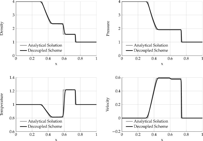
Figure 1: The black lines are the simulation results and the gray lines are the analytical resolutions .These are the results at the 180th step, i.e. the time $t\!=\!0.1504$. The specific heat ratio is $\gamma\!=\!1.4$ and the relaxation time is $\tau\!=\!2/3$. The initial condition of the left side is ${\rho\!=\!4,T\!=\!1,\bm{u}\!=\!0}$ and that of the right side is ${\rho\!=\!1,T\!=\!1,\bm{u}\!=\!0}$.

Tab(3) gives the relative error of density $\rho$, pressure $p$, absolute temperature $T$ and the velocity $u$. The relative error is defined as

$$Error=\frac{\displaystyle\sum_{i}|x_{nume,i}-x_{anal,i}|}{\displaystyle\sum_{i}|x_{anal,i}|},$$ (32)

where $x_{nume}$ is the numerical solutions, $x_{anal}$ is the analytical solutions and $i=X+1$. Tab(3) shows that the maximum of relative error is $2.42\%$. This relative error is acceptable.

Table 3: Relative error of the numerical solutions.

	$\rho$	$p$	$T$	$u_{x}$
$Error$	$0.0077$	$0.0055$	$0.0064$	$0.0242$

VII Conclusion

This work proposes a way based on the Hermite expansion to construct LB schemes for the compressible Navier-Stokes equations with arbitrary specific heat ratio. The equilibrium distribution function $f^{eq}(\bm{\xi},\eta)$, the distribution function $f(\bm{\xi},\eta)$ and the evolution function are decoupled into two parts, namely one is in relation to the translational velocity $\bm{\xi}$ and the other is connected with the rotational velocity $\eta$. The two evolution equations evolve separately. The translational velocity $\bm{\xi}$ is discretized in a two- or three- dimensional LB model and the rotational velocity $\eta$ is discretized in another one-dimensional LB model. The Hermite expansion is applied to deriving these two LB models. The correct flexible specific heat ratio is obtained and correct relation between the temperature $T$ and the internal energy $E$ is derived via the Chapman-Enskog expansion. The decoupled scheme is validated by a shock tube simulation. The simulation results agree with the analytical resolutions very well.

The LB models used in the decoupled scheme is same as the ones used in the schemes with fixed specific heat ratio. It is not necessary for the decoupled scheme to construct new LB models specially. The models with fixed specific heat ratio can applied to the decoupled scheme without any recommendation. This is different from the existing schemes which construct new models in order to adjust the specific heat ratio.

The decoupled scheme proposed by this work can make use of the models constructed via the Hermite expansion, so the process of constructing new schemes is simple and higher-order accuracy can be achieved easily. For the same reason, the decoupled scheme is more stable than the schemes constructed by the early way, which derives LB models via a try-error method.

*

Appendix A Derivation of the Navier-Stokes equations from the evolution equations of $g(\bm{\xi})$ and $h({\eta})$ via the Chapman-Enskog expansion

In this appendix, we derive the Navier-Stokes equations with flexible specific heat ratio from the evolution equations of $g(\bm{\xi})$ and $h({\eta})$ via the Chapman-Enskog expansion.

Expanding the distribution functions $g_{i}$ and $h_{j}$, the derivatives of the time $t$ and the space in terms of the Kundsen number $\epsilon$ we obtain

$$\nabla= \epsilon\nabla_{1},$$ (33a)

$$\frac{\partial}{\partial t}=\epsilon\frac{\partial}{\partial t_{1}} +\epsilon^{2}\frac{\partial}{\partial t_{2}},$$ (33b)

$$g_{i}=g_{i}^{(0)}+\epsilon g_{i}^{(1)}+\epsilon^{2}g_{i}^{(2)},$$ (33c)

$$h_{j}=h_{j}^{(0)}+\epsilon h_{j}^{(1)}+\epsilon^{2}h_{j}^{(2)}.$$ (33d)

Substituting Formula(33c) into the evolution equation of the translational velocity, i.e. Formula(18a) and comparing the order of $\epsilon$ we obtain

$$g_{i}^{(0)}=g_{i}^{(eq)},$$ (34a)

$$(\frac{\partial}{\partial t_{1}}+ \bm{\xi}_{i}\cdot\nabla_{1})g_{i}^{(0)}+\frac{1}{\tau}g_{i}^{(1)}=0,$$ (34b)

$$\frac{\partial g_{i}^{(0)}}{\partial t_{2}}+(\frac{\partial}{\partial t_{1}} +\bm{\xi}_{i}\cdot\nabla_{1})g_{i}^{(1)}+\frac{1}{\tau}g_{i}^{(2)}=0.$$ (34c)

Considering the discrete form of Formula(11) in the discrete velocity space

$$\sum_{i}g_{i}= \sum_{i}g_{i}^{eq}=\rho,$$ (35a)

$$\sum_{i}g_{i}= \sum_{i}g_{i}^{eq}=\rho\bm{u},$$ (35b)

$$\sum_{i}g_{i}\frac{1}{2}\xi_{i}^{2}= \sum_{i}g_{i}^{eq}\frac{1}{2}\xi_{i}^{2}=\rho(\frac{1}{2}u^{2}+e_{t}),$$ (35c)

we obtain

$$\sum_{i}g_{i}^{(n)}=0,\sum_{i}g_{i}^{(n)}\bm{\xi}_{i}=0,\sum_{i}g_{i}^{(n)}\frac{1}{2}\xi_{i}^{2}=0,\quad n=1,2.$$ (36)

Substituting Formula(33d) into the evolution equation of the rotational velocity,i.e.Formula(18b) and comparing the order of $\epsilon$ we obtain

$$h_{j}^{(0)}=h_{j}^{(eq)},$$ (37a)

$$(\frac{\partial}{\partial t_{1}}+ \bm{u}\cdot\nabla_{1})h_{j}^{(0)}+\frac{1}{\tau}h_{j}^{(1)}=0,$$ (37b)

$$\frac{\partial h_{j}^{(0)}}{\partial t_{2}}+(\frac{\partial}{\partial t_{1}} +\bm{u}\cdot\nabla_{1})h_{j}^{(1)}+\frac{1}{\tau}h_{j}^{(2)}=0.$$ (37c)

Considering the discrete form of Formula(12) in the discrete velocity space

$$\sum_{j}h_{j}= \sum_{j}h_{j}^{eq}=1,$$ (38a)

$$\sum_{j}h_{j}\frac{n}{2}\eta_{j}^{2}= \sum_{j}h_{j}^{eq}\frac{n}{2}\eta_{j}^{2}=e_{r},$$ (38b)

we obtain

$$\sum_{j}h_{j}^{(n)}=0,\sum_{j}h_{j}^{(n)}\frac{n}{2}\eta^{2}_{j}=0,\quad n=1,2.$$ (39)

Some velocity moments of $g_{i}$ and $h_{j}$ will be used in the derivation of the Navier-Stokes equations and we list them as fellow

$$\sum_{i}g_{i}^{eq}= \rho,$$ (40a)

$$\sum_{i}g_{i}^{eq}\bm{\xi}_{i}= \rho\bm{u},$$ (40b)

$$\sum_{i}g_{i}^{eq}\bm{\xi}_{i}\bm{\xi}_{i}= \rho\bm{u}\bm{u}+P\bm{\delta},$$ (40c)

$$\sum_{i}g_{i}^{eq}\bm{\xi}_{i}\bm{\xi}_{i}\bm{\xi}_{i}= \rho\bm{u}\bm{u}\bm{u}+P\bm{u}\bm{\delta},$$ (40d)

$$\sum_{i}g_{i}^{eq}\frac{1}{2}\xi_{i}^{2}= \rho(\frac{1}{2}u^{2}+e_{t}),$$ (40e)

$$\sum_{i}g_{i}^{eq}\frac{1}{2}\xi_{i}^{2}\bm{\xi}_{i}= \rho(\frac{1}{2}u^{2}+e_{t})\bm{u},$$ (40f)

$$\sum_{i}g_{i}^{eq}\frac{1}{2}\xi_{i}^{2}\bm{\xi}_{i}\bm{\xi}_{i}= P(\frac{2}{D}e_{t}+\frac{1}{2}u^{2}+e_{t})\bm{\delta},$$

$$+(2P+\frac{1}{2}\rho u^{2}+\rho e_{t})\bm{u}\bm{u},$$ (40g)

where $P\bm{u}\bm{\delta}=P(u_{r}\delta_{st}+u_{s}\delta_{tr}+u_{t}\delta_{rs})$. Here, the Grad notes is usedGrad (1949). Two velocity moments of $h_{j}$ will be used in the following parts

$$\sum_{j}h_{j}^{eq} =1,$$ (41a)

$$\sum_{j}h_{j}^{eq}\frac{n}{2}\eta^{2} =e_{r}.$$ (41b)

A.1 Derivation of the continuity equation

Taking the zeroth order moment of Formula(34b), we obtain

$$\sum_{i}(\frac{\partial}{\partial t_{1}}+\bm{\xi}_{i}\cdot\nabla_{1})g_{i}^{(0)}+\frac{1}{\tau}\sum_{i}g_{i}^{(1)}=0$$ (42)

Substituting Formula(36) and (40) into (42), the continuity equation of the first order is obtained

$$\frac{\partial}{\partial t_{1}}\rho+\nabla_{1}\cdot\rho\bm{u}=0.$$ (43)

Taking the zeroth order moment of Formula(34c), we obtain

$$\frac{\partial\sum_{i}g_{i}^{(0)}}{\partial t_{2}}+\sum_{i}(\frac{\partial}{\partial t_{1}}+\bm{\xi}_{i}\cdot\nabla_{1})g_{i}^{(1)}+\frac{1}{\tau}\sum_{i}g_{i}^{(2)}=0.$$ (44)

Substituting Formula(36) and (40) into (44), then summing on $i$ we obtain the continuity equation of the second order

$$\frac{\partial\rho}{\partial t_{2}}=0.$$ (45)

Making use of Formula(33b) and combining the continuity equation of the first and second order, i.e. Formula(43) and (45), the continuity equation is obtained

$$\frac{\partial}{\partial t}\rho+\nabla\cdot\rho\bm{u}=0.$$ (46)

A.2 Derivation of the momentum
conservation equation

Taking the first order moment of Formula(34b)

$$\sum_{i}(\frac{\partial}{\partial t_{1}}+\bm{\xi}_{i}\cdot\nabla_{1})g_{i}^{(0)}\bm{\xi}_{i}+\frac{1}{\tau}\sum_{i}g_{i}^{(1)}\bm{\xi}_{i}=0,\\$$ (47)

and inserting Formula(36) and (40), we get the conservation momentum equation of the first order

$$\frac{\partial}{\partial t_{1}}\rho\bm{u}+\nabla_{1}\cdot(\rho\bm{u}\bm{u}+P\bm{\delta})=0.\\$$ (48)

Taking the first order moment of Formula(34c)

$$\frac{\partial\sum_{i}g_{i}^{(0)}\bm{\xi}_{i}}{\partial t_{2}}+\sum_{i}(\frac{\partial}{\partial t_{1}}+\bm{\xi}_{i}\cdot\nabla_{1})g_{i}^{(1)}\bm{\xi}_{i}+\frac{1}{\tau}\sum_{i}g_{i}^{(2)}\bm{\xi}_{i}=0,$$ (49)

substituting Formula(34b) into (49) and simplifying, we obtain

$$\frac{\partial\sum_{i}g_{i}^{(0)}\bm{\xi}_{i}}{\partial t_{2}}-\tau\nabla_{1}\cdot (\frac{\partial}{\partial t_{1}}\sum_{i}\bm{\xi}_{i}\bm{\xi}_{i}g_{i}^{(0)}$$

$$+\nabla_{1}\cdot\sum_{i}\bm{\xi}_{i}\bm{\xi}_{i}\bm{\xi}_{i}g_{i}^{(1)})=0.$$ (50)

Inserting the moments of $g_{i}$ i.e. Formula(40), into Formula(A.2) we obtain

$$\frac{\partial\rho\bm{u}}{\partial t_{2}}-\tau\nabla_{1}\cdot[\frac{\partial}{\partial t_{1}}(\rho\bm{u}\bm{u}+P\bm{\delta})+\nabla_{1}\cdot\sum_{i}\bm{\xi}_{i}\bm{\xi}_{i}\bm{\xi}_{i}g_{i}^{(1)}]=0,$$ (51)

where $\displaystyle\frac{\partial P}{\partial t_{1}}$ is a difficult point to simplify. To simplify $\displaystyle\frac{\partial P}{\partial t_{1}}$, we should obtain the energy conservation equation of the first order firstly.

Multiplying $\displaystyle\frac{1}{2}\xi^{2}_{i}$ to Formula(34b) and summing on $i$ we obtain

$$\sum_{i}(\frac{\partial}{\partial t_{1}}+\bm{\xi}_{i}\cdot\nabla_{1})g_{i}^{(0)}\frac{1}{2}\xi^{2}_{i}+\frac{1}{\tau}\sum_{i}g_{i}^{(1)}\frac{1}{2}\xi^{2}_{i}=0.$$ (52)

Substituting the moments of $\bm{\xi}_{i}$ i.e. Formula(40), into Formula(52), we obtain the translational internal energy conversation equation of the first order

$$\frac{\partial}{\partial t_{1}}(\frac{1}{2}\rho u^{2}+\rho e_{t})+\nabla_{1}\cdot(\frac{1}{2}\rho u^{2}+\rho e_{t}+P)\bm{u}=0.$$ (53)

Multiplying $\displaystyle\frac{1}{2}\eta^{2}$ to Formula(37b), summing on $j$ and inserting the moments of $h_{j}$ ,i.e. Formula(41), we obtain the rotational internal energy conversation equation of the first order in nonconservation form

$$\frac{\partial}{\partial t_{1}}e_{r}+\bm{u}\cdot\nabla_{1}e_{r}=0.$$ (54)

Multiplying $\rho$ to Formula(54) and multiplying $e_{r}$ to Formula(43), then adding up we obtain

$$\rho(\frac{\partial}{\partial t_{1}}e_{r}+\bm{u}\cdot\nabla_{1}e_{r})+e_{r}(\frac{\partial}{\partial t_{1}}\rho+\nabla_{1}\cdot\rho\bm{u})=0.$$ (55)

Simplifying Formula(55) we obtain the rotational internal conversation energy equation of the first order in conservation form

$$\frac{\partial}{\partial t_{1}}\rho e_{r}+\nabla_{1}\cdot\rho\bm{u}e_{r}=0.$$ (56)

Combining the translational internal energy conversation equation of the first order Formula(53) and the rotational internal energy conversation equation of the first order formula(56), we obtain the energy conversation equation of the first order

$$\frac{\partial}{\partial t_{1}}(\frac{1}{2}\rho u^{2}+\rho E)+\nabla_{1}\cdot(\frac{1}{2}\rho u^{2}+\rho E+P)\bm{u}=0.$$ (57)

Substituting $P=\displaystyle\frac{2}{D+n}\rho E$ into Formula(57) we obtain

$$\frac{\partial}{\partial t_{1}}(\frac{1}{2}\rho u^{2}+\frac{D+n}{D}P)+\nabla_{1}\cdot(\frac{1}{2}\rho u^{2}+\frac{D+n+2}{D}P)\bm{u}=0.$$ (58)

Expanding Formula(58), substituting (43) and (48) into it, after some algebra, we obtain

$$\frac{\partial P}{\partial t_{1}}=-\nabla_{1}\cdot P\bm{u}-\frac{2}{D+n}P\nabla_{1}\cdot\bm{u},$$ (59)

Substituting Formula(59) into (51), after some algebra, we obtain the momentum conversation equation of the second order

$$\frac{\partial}{\partial t_{2}}\rho\bm{u}=\nabla_{1}\cdot\frac{2}{D}\rho e_{t}\tau[(\nabla_{1}\bm{u}+\bm{u}\nabla_{1})-\frac{2}{D+n}\nabla_{1}\cdot\bm{u}\bm{\delta}].$$ (60)

Combining the momentum equation of the first order and second order, we obtain the moment conversation equation

$$\frac{\partial}{\partial t}\rho\bm{u}+\nabla\cdot(\rho\bm{u}\bm{u}+P\bm{\delta})=\nabla\cdot\mu[(\nabla\bm{u}+\bm{u}\nabla)-\frac{2}{D+n}\nabla\cdot\bm{u}\bm{\delta}],\\$$ (61)

where $\mu=\displaystyle\frac{2}{D}\rho e_{t}\tau$ is the dynamic viscosity coefficient.

A.3 Derivation of the energy conversation equation

We have obtained the energy conversation equation of the first order, i.e. Formula(57),

$$\frac{\partial}{\partial t_{1}}(\frac{1}{2}\rho u^{2}+\rho E)+\nabla_{1}\cdot(\frac{1}{2}\rho u^{2}+\rho E+P)\bm{u}=0.$$

Now, we derive the energy conversation equation of the second order.

Multiplying $\displaystyle\frac{1}{2}\xi_{i}^{2}$ to Formula(34c), substituting (34b) into it, and summing on $i$, we obtain

$$\frac{\partial}{\partial t_{2}}\sum_{i}g_{i}^{(0)}\frac{1}{2}\xi_{i}^{2}=\nabla_{1}\cdot\tau(\frac{\partial}{\partial t_{1}} \sum_{i}g_{i}^{(0)}\frac{1}{2}\xi^{2}_{i}\bm{\xi}_{i}$$

$$+ \nabla_{1}\cdot g_{i}^{(0)}\bm{\xi}_{i}\bm{\xi}_{i}\frac{1}{2}\xi^{2}_{i})$$ (62)

Substituting the moments of $g_{i}$ into Formula(A.3), we obtain

$$\frac{\partial}{\partial t_{2}} (\frac{1}{2}\rho u^{2}+e_{t})=\nabla_{1}\cdot\tau[\frac{\partial}{\partial t_{1}}(\frac{1}{2}\rho u^{2}+e_{t}+P)\bm{u}$$

$$+ \nabla_{1}\cdot P(\frac{2}{D}e_{t}+\frac{1}{2}u^{2}+e_{t})\bm{\delta}+(2P+\frac{1}{2}\rho u^{2}+e_{t})\bm{u}\bm{u}]$$ (63)

Inserting Formula (43) , (48), (58) and (59) into Formula(A.3), after some algebra, we get the translational internal energy conversation equation of the second order

$$\frac{\partial}{\partial t_{2}}(\frac{1}{2}\rho u^{2}+e_{t})=\nabla_{1}\cdot\tau P\bm{u}[(\nabla_{1}\bm{u}+\bm{u}\nabla_{1})$$

$$-\frac{2}{D+n}\nabla_{1}\bm{u}\bm{\delta}]+\nabla_{1}\cdot\tau P\frac{D+2}{D}\nabla_{1}e_{t}.$$ (64)

Multiplying $\displaystyle h_{j}^{(0)}$ to Formula(34c), Multiplying $\displaystyle g_{i}^{(0)}$ to Formula(37c) and adding them up

$$\frac{\partial}{\partial t_{2}}g_{i}^{(0)}h_{j}^{(0)} +(\frac{\partial}{\partial t_{1}}+\xi\cdot\nabla_{1})g_{i}^{(1)}h_{j}^{(0)}$$

$$+(\frac{\partial}{\partial t_{1}}+ \bm{u}\cdot\nabla_{1})g_{i}^{(0)}h_{j}^{(1)}+\frac{1}{\tau}(g_{i}^{(2)}h_{j}^{(0)}+g_{i}^{(0)}h_{j}^{(2)})=0,$$ (65)

substituting Formula(34b) into (A.3), we get

$$\frac{\partial}{\partial t_{2}}g_{i}^{(0)}h_{j}^{(0)} -\nabla_{1}\cdot\tau(\frac{\partial}{\partial t_{1}}\bm{\xi}_{i}g_{i}^{(0)}h_{j}^{(0)}+\nabla_{1}\cdot\bm{\xi}_{i}\bm{\xi}_{i}g_{i}^{(0)}h_{j}^{(0)})$$

$$+(\frac{\partial}{\partial t_{1}}+ \bm{u}\cdot\nabla_{1})g_{i}^{(0)}h_{j}^{(1)}+\frac{1}{\tau}(g_{i}^{(2)}h_{j}^{(0)}+g_{i}^{(0)}h_{j}^{(2)})=0.$$ (66)

Multiplying $\displaystyle\frac{n}{2}\eta^{2}$ to Formula(A.3) and summing on $i$ and $j$ we obtain

$$\frac{\partial}{\partial t_{2}}\rho e_{r}=\nabla_{1}\cdot\tau[\frac{\partial}{\partial t_{1}}\rho\bm{u}e_{r}+\nabla_{1}\cdot(\rho\bm{u}\bm{u}+P\bm{\delta})e_{r}].$$

Inserting Formula(48) and (56) into (A.3), after some algebra, we obtain the rotational internal energy conversation equation of the second order

$$\frac{\partial}{\partial t_{2}}\rho e_{r}=\nabla_{1}\cdot\tau\rho e_{t}\frac{n}{D}\nabla_{1}e_{r}.$$ (68)

Combining the rotational internal energy conversation equation of the seconde order Formula(68) with the translational internal conversation energy of the seconde order Formula(A.3), we obtain the energy conversation equation of the second order

$$\frac{\partial}{\partial t_{2}} (\frac{1}{2}\rho u^{2}+\rho E)=\nabla_{1}\cdot\tau P\bm{u}[(\nabla_{1}\bm{u}+\bm{u}\nabla_{1})$$

$$-\frac{2}{D+n}\nabla_{1}\bm{u}\bm{\delta}]+\nabla_{1}\cdot\frac{D+n+2}{D}\tau\rho e_{t}\nabla_{1}e_{t}.$$ (69)

Combining the energy conversation equation of the second order (A.3) with the energy conversation equation of the first order Formula(57) we obtain the energy conversation equation

$$\frac{\partial}{\partial t}\rho (E+\frac{1}{2}u^{2})+\nabla\cdot\rho\bm{u}(E+\frac{1}{2}u^{2}+\frac{P}{\rho})$$

$$= \nabla\cdot\mu\bm{u}(\nabla\bm{u}+\bm{u}\nabla-\frac{2}{D}\nabla\cdot\bm{u}\delta)+\nabla\cdot\kappa\nabla E$$ (70)

where

$$P=\frac{2}{D}\rho e_{t},\mu=\frac{2}{D}\rho e_{t}\tau,\kappa=\frac{2(D+n+2)}{D(D+n)}\rho e_{t}\tau.$$ (71)

Formula(A.3) is the energy conversation equation with flexible specific heat ratio and the specific heat ratio $\gamma$ is

$$\gamma=\frac{D+n+2}{D+n}.$$

The specific heat ratio $\gamma$ can be adjusted by changing the free degree of the rotational velocity $n$.

References

• Chen et al. (1992) S. Chen, Z. Wang, X. Shan,  and G. D. Doolen, Journal of Statistical Physics 68, 379 (1992).
• Chen and Doolen (1998) S. Chen and G. D. Doolen, Annual review of fluid mechanics 30, 329 (1998).
• Shi et al. (2001) W. Shi, W. Shyy,  and R. Mei, Numerical Heat Transfer: Part B: Fundamentals 40, 1 (2001).
• Kataoka and Tsutahara (2004) T. Kataoka and M. Tsutahara, Physical review E 69, 035701 (2004).
• Watari (2007) M. Watari, Physica A: Statistical Mechanics and its Applications 382, 502 (2007).
• Tsutahara et al. (2008) M. Tsutahara, T. Kataoka, K. Shikata,  and N. Takada, Computers & Fluids 37, 79 (2008).
• Philippi et al. (2006) P. C. Philippi, L. A. Hegele Jr, L. O. Dos Santos,  and R. Surmas, Physical Review E 73, 056702 (2006).
• Philippi et al. (2015) P. Philippi, D. Siebert, L. Hegele Jr,  and K. Mattila, Journal of the Brazilian Society of Mechanical Sciences and Engineering , 1 (2015).
• Shan et al. (2006) X. Shan, X.-F. Yuan,  and H. Chen, Journal of Fluid Mechanics 550, 413 (2006).
• Mattila et al. (2014) K. K. Mattila, L. A. Hegele Júnior,  and P. C. Philippi, The Scientific World Journal 2014 (2014).
• Shim (2013a) J. W. Shim, Physical Review E 88, 053310 (2013a).
• Shim (2013b) J. W. Shim, Physical Review E 87, 013312 (2013b).
• Ansumali et al. (2003) S. Ansumali, I. V. Karlin,  and H. C. Öttinger, EPL (Europhysics Letters) 63, 798 (2003).
• Chikatamarla and Karlin (2006) S. S. Chikatamarla and I. V. Karlin, Physical review letters 97, 190601 (2006).
• Chikatamarla and Karlin (2009) S. S. Chikatamarla and I. V. Karlin, Physical Review E 79, 046701 (2009).
• Yudistiawan et al. (2010) W. P. Yudistiawan, S. K. Kwak, D. Patil,  and S. Ansumali, Physical Review E 82, 046701 (2010).
• Xu et al. (2014) A. Xu, G. Zhang, Y. Li,  and H. Li, Progress in Physics 34 (2014).
• Shan et al. (2010) X. Shan et al., Physical Review E 81, 036702 (2010).
• Sod (1978) G. A. Sod, Journal of Computational Physics 27, 1 (1978).
• Grad (1949) H. Grad, Communications on Pure and Applied Mathematics 2, 325 (1949).