Line shapes and time dynamics of the Förster resonances between two Rydberg atoms in a time-varying electric field
Abstract
The observation of the Stark-tuned Förster resonances between Rydberg atoms excited by narrowband cw laser radiation requires usage of a Stark-switching technique in order to excite the atoms first in a fixed electric field and then to induce the interactions in a varied electric field, which is scanned across the Förster resonance. In our experiments with a few cold Rb Rydberg atoms we have found that the transients at the edges of the electric pulses strongly affect the line shapes of the Förster resonances, since the population transfer at the resonances occurs on a time scale of 100 ns, which is comparable with the duration of the transients. For example, a short-term ringing at a certain frequency causes additional radio-frequency-assisted Förster resonances, while non-sharp edges lead to asymmetry. The intentional application of the radio-frequency field induces transitions between collective states, whose line shape depends on the interaction strengths and time. Spatial averaging over the atom positions in a single interaction volume yields a cusped line shape of the Förster resonance. We present a detailed experimental and theoretical analysis of the line shape and time dynamics of the Stark-tuned Förster resonances for two Rb Rydberg atoms interacting in a time-varying electric field.
pacs:
32.80.Ee, 32.70.Jz , 32.80.Rm, 34.10.+xI Introduction
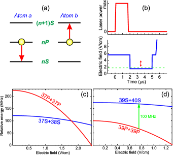
Long-range interactions between highly excited Rydberg atoms are of interest for quantum information processing with single neutral atoms [1,2]. Resonant dipole-dipole interaction between atoms in an identical nL Rydberg state can be implemented via Stark-tuned Förster resonances [3,4]. A Rydberg state should be exactly midway between two other Rydberg states of the opposite parity [Fig. 1(a)] to induce a Förster resonance. The electric field corresponding to the Förster resonance has certain values defined by the polarizabilities and energy spacing of Rydberg states in a zero field. Upon appropriate experimental conditions (highly stable and homogeneous electric field, absence of stray electric fields, weak dipole-dipole interaction), Stark-tuned Förster resonances can be as narrow as a few millivolts per centimeter [5].
In our earlier papers [6-8] we studied the line shape of the Förster resonance in cold Rb Rydberg atoms excited by a broadband pulsed laser radiation via a three-photon transition. The resonance was recorded by slowly scanning a weak electric field near the resonant value of 1.79 V/cm [Fig. 1(c)]. When the field was scanned by 0.2 V/cm, the frequency of the optical transition on the third excitation step changed by tens of megahertz due to the Stark effect. This frequency change was unimportant for broadband pulsed radiation as the radiation line width was much broader (10 GHz). However, an electric-field pulse was applied at the moment of laser excitation to pull out the cold Rb photoions formed due to photoionization by the intense pulsed laser radiation; otherwise, the Förster resonance became asymmetrical due to inhomogeneous electric fields from the photoions [8].
In our recent experiments [2,9,10] we have switched to three-photon excitation by narrowband cw lasers. This prevents the appearance of photoions, since the laser intensities used are much lower than those for pulsed excitation, and the pulling electric-field pulse is not required. However, scanning the electric field by just 50 mV/cm shifts the Rydberg level out of resonance with the laser radiation, as the cw lasers have line widths below 1 MHz [9]. In order to avoid this problem, one needs to apply a Stark-switching technique [11-14] to excite the atoms first in a fixed electric field and then to induce the interactions in a lower electric field, which is scanned across the Förster resonance [10,13], as shown in Fig. 1(b).
We have found that the transients at the edges of the controlling electric pulses strongly affect the line shapes of the Förster resonances, since the population transfer at the resonances occurs on a time scale of 100 ns, which is comparable with the duration of the transients. For example, a short-term ringing at a certain frequency causes additional radio-frequency (rf)-assisted Förster resonances, while non-sharp edges lead to asymmetry (see Fig. 3). The short-time scale of the Rydberg interactions between cold atoms was also observed in Refs. [15,16].
In this paper, we present a detailed experimental and theoretical analysis of the Förster resonance line shapes and time dynamics in a time-varying electric field used for the Stark switching. The resonance under study is the Förster resonant energy transfer due to dipole-dipole interaction of two Rb Rydberg atoms [Fig. 1(a)] in a small single laser excitation volume of a frozen Rydberg gas. The energy detuning of this resonance, , is controlled by a weak dc electric field . The energy shift of a Rydberg level with nonzero quantum defect is quadratic and is defined by its polarizability, . The detuning is then given by
| (1) |
Here, is the detuning in a zero electric field (for example, 103 MHz for n=37 and +74 MHz for n=39). The detuning can be tuned to zero for Rydberg states with , as shown in Fig. 1(c) for the state, while for states with , the dc electric field only increases , as shown in Fig. 1(d) for the state. For the latter, a Förster resonance can be obtained by adding a 100 MHz rf field that induces rf transitions between collective states and compensates for the Förster energy defect, as demonstrated in our recent paper [10].
An experimental and theoretical line-shape analysis of the Stark-tuned Förster resonances was performed in Ref. [17] for the case of potassium Rydberg atoms colliding in a thermal atomic beam. It was found that averaging over atomic velocities leads to a cusped line shape, while resonant collisions in a velocity-selected atomic beam have nearly Lorentzian line shape. This finding agrees with what we have observed in a similar experiment on resonant Rydberg collisions in a sodium thermal atomic beam [18].
It is quite surprising that cusp-shaped Förster resonances are also observed in cold Rydberg atom gases, where the atoms are nearly frozen [19,20]. Line-shape analysis was performed in several papers. In Ref. [21], it was found theoretically that the rare pair fluctuation at small spatial separation is the dominant factor contributing to the broadening of the Förster resonances. Our numerical Monte Carlo simulations using the Schrödinger’s equation [7,22] and our experimental data [7,10] have shown that spatial averaging over the random positions of Rydberg atoms interacting in a single laser excitation volume results in cusp-shaped Förster resonances as soon as the resonances saturate and the interaction time is long enough. Cusp-shaped Förster resonances were also observed recently at high Rb Rydberg atom density in Ref. [23] and an analytical model has been proposed. Another recent paper [24] reports on the broadening and overlapping of the Förster resonances in Rb Rydberg atoms at high density. Quasi-forbidden Förster resonances in Cs Rydberg atoms were observed in Ref. [25]. Finally, in Ref. [26], microwave pump-probe experiments also demonstrated cusped line shapes observed in the spectra of dipole-dipole broadened microwave transitions in Rb Rydberg atoms. The line-shape analysis of the resonant dipole-dipole interaction thus remains a hot topic in the study of cold Rydberg atom samples.
II Experimental setup
The experiments are performed with cold 85Rb atoms in a magneto-optical trap (MOT). Typically, 10 atoms are trapped in a cloud of 0.50.6 mm diameter. Our experiments feature atom-number-resolved measurement of the signals obtained from detected Rydberg atoms with a detection efficiency of 65% [7]. It is based on a selective field ionization (SFI) detector with channel electron multiplier (CEM) and post-selection technique. We can record Förster resonances for up to five of the detected Rydberg atoms and compare these with the numerical Monte Carlo simulations.
The electric field for SFI is formed by two stainless-steel plates that are 1 cm apart. These plates have holes and meshes for passing the vertical cooling laser beams and the electrons to be detected. The CEM output pulses from the nS and [nP+(n+1)S] states (the two latter states have nearly identical ionizing fields and are detected together) are detected with two independent gates and sorted according to the number N of the totally detected Rydberg atoms. The normalized N-atom signals are the fractions of atoms that have undergone a transition to the final nS state.
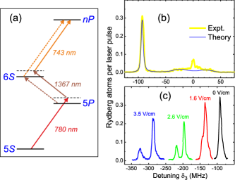
The excitation of Rb atoms to the nP3/2(|MJ|=1/2) Rydberg states is realized via three-photon transition [Fig. 2(a)] by means of three cw lasers modulated to form 2 s exciting pulses at a repetition rate of 5 kHz [9]. The first excitation step is blue detuned by =+92 MHz from the transition in 85Rb atoms. The second step is on-resonance (=0) with the transition. By scanning the frequency of the third-step laser across the transition, we observe a strong narrow peak of the coherent three-photon excitation [solid arrows in Fig. 2(a)] detuned by =92 MHz [Fig. 2(b)], while the incoherent three-step excitation [dashed arrows in Fig. 2(a)] is almost absent, as discussed in our papers [2,9]. The intermediate states and are thus almost not populated.
Small Rydberg excitation volume of 2040 m in size is formed using crossed laser-beam geometry [6]. The effective volume size can be controlled by changing the laser intensity on the second excitation step (higher intensity gives bigger volume). The intensity is measured by observing the Autler-Townes splitting of the state for the incoherent three-step excitation [small peaks at 26 MHz in Fig. 2(b)]. The small peak at =0 in Fig. 2(b) is a zero reference due to the added cooling laser radiation on the first step. The blue (thin) lines in Fig. 2(b) are theoretical calculations in a four-level model taking into account the finite laser line widths [9]. Application of a weak electric field shifts and splits the three-photon resonance, as shown in Fig. 2(c). This allows us to use the Stark-switching technique to control the interaction of Rb atoms with the laser radiations.
The laser intensities are adjusted to obtain about one Rydberg atom excited per laser pulse on average. A proper choice of the exciting laser polarization (along the dc electric field) provides excitation of only nP3/2(|MJ|=1/2) atoms from the intermediate state. In this case, a single Förster resonance is observed, which is most appropriate for experimental and theoretical analysis.
The dc electric field is calibrated with 0.2% uncertainty using the Stark spectroscopy of the microwave transition 37P3/2 37S1/2 at 80.124 GHz [6,8]. The MOT magnetic field is not switched off in order to have high repetition rate, but microwave probing on the same transition allowed us to align the excitation point to a nearly zero magnetic field [6]. The 780 nm cooling laser beams are switched off before Rydberg excitation and then switched on after the SFI detection of Rydberg atoms.
We use a Stark-switching technique [10-13] to switch the Rydberg interactions on and off, as depicted in Fig. 1(b). Laser excitation occurs during 2 s at a fixed electric field of 5.6 V/cm. Then the field decreases to a lower value near the resonant electric field (1.79 V/cm for the 37P3/2 state), which acts for 3 s or less until the field increases back to 5.6 V/cm. Then, 0.5 s later, a ramp of the strong field-ionizing electric pulse of 200 V/cm is applied. The lower electric field is slowly scanned across the Förster resonance and the SFI signals are accumulated for laser pulses. A pulse of the rf field with variable amplitude ( V/cm) and frequency ( MHz) can be admixed to the lower dc field.
III Effect of the edges of the electric-field pulse
The usage of the Stark-switching technique requires studying the effect of the finite duration of the edges and of the electric-field pulse itself on the observed line shape of the Förster resonance. As noted in Refs. [15,16], population transfer at a Förster resonance may occur rapidly, on a time scale of 100 ns. If the edges have similar duration, these can affect the line shape, which under conditions should be symmetrical and close to Lorentzian, except for the wings of the resonance [7]. At the same time, too fast switching may cause non-adiabatic transitions between Rydberg states, so the edges must not be too short (longer than 1 ns).
In our first experiments on the Stark switching of the Förster resonance , we revealed that when we tried to obtain the 10-ns edges, on the leading edge there appeared a 300 ns transient in the form of damped 20 MHz oscillations of the voltage. It resulted in the appearance of additional weaker and broader Förster resonances having a regular structure of repetitions with the frequency interval being also about 20 MHz [Fig. 3(a)]. In fact, these resonances were induced by the pulse of the radio-frequency (rf) field corresponding to the ringing.
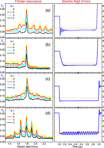
Then we suppressed the ringing and increased the leading edge duration to approximately 100 ns, while the falling edge was shorter (30 ns). The usage of such pulse with asymmetric edges has led to a noticeable asymmetry in the line shape of the Förster resonance [Fig. 3(b)]. This can be understood from the fact that in our experimental conditions, the population transfer at Förster resonance occurs mainly during the long leading edge.
After a substantial improvement of the electric circuitry, we managed to obtain an electric pulse with short edges (10 ns) and without any noticeable ringing or transients. This allowed us to record the symmetrical spectrum of the Förster resonance at Stark switching [Fig. 3(c)], which is suitable for comparison with theory.
Finally, the intentional application of a 100 mV rf-field at 15 MHz induced additional Förster resonances [Fig. 3(d)], which are rf-assisted resonances of various orders, as shown in the scheme in Fig. 6(a) for the energy levels of the initial 37P+37P and final 37S+38S collective states in dc electric field. We studied these resonances experimentally in Ref. [10].
In all cases considered above, the Förster resonance amplitudes and widths grow as the number of atoms N increases from 2 to 5, due to an increase in the total interaction energy and density of Rydberg atoms in the same laser excitation volume. The cusp-shaped Förster resonances are formed as soon as the resonances saturate and the interaction time is long enough. This observation agrees with our previous theoretical Monte Carlo simulations of the Förster resonances for Rb Rydberg atoms randomly placed in a single excitation volume [7,22].
IV Time dynamics of the Förster resonances
IV.1 Theory with density-matrix equations
The next issue to be analyzed is the dependence of the line shape and amplitude of the Förster resonance on the interaction time t which is set by the length of the controlling electric-field pulse [Fig. 3(c)]. We consider an example of the Stark-tuned Förster resonance for two Rb Rydberg atoms [see Fig. 1(a) for the energy level and transition scheme] randomly placed in a single excitation volume. The initial energy detuning in a zero electric field is 103 MHz. For the laser-excited 37P3/2(|MJ|=1/2) Rydberg atoms a single Förster resonance is observed at 1.79 V/cm, as shown in Fig. 3(c).
Our Förster resonance induces transitions between Rydberg states with . This corresponds to the z-oriented dipoles, and the operator of the dipole-dipole interaction is
| (2) |
where are the z components of the dipole-moment operators of the two interacting atoms a and b, is the z component of the vector connecting the two atoms (z axis is chosen along the dc electric field), and is the dielectric constant.
In order to calculate the time evolution of the populations in the two Rydberg atoms interacting via a Förster resonance, the simplest way is to solve the Schrödinger’s equation for two interacting atoms. For two motionless atoms, this equation is solved analytically. Then the Förster resonance line shape and time dynamics can be obtained by Monte Carlo spatial averaging of the random atom positions in the laser excitation volume, as we did in Refs. [7,22].
However, when comparing the experimental and theoretical line shapes in Ref. [7], we have found that in the experiment, we observed additional broadening of the Förster resonance, which was not described by the Schrödinger’s equation for three-level Rydberg atoms shown in Fig. 4(a). The additional broadening was due to the unresolved hyperfine structure of Rydberg states not taken into account in theory (500 kHz) and due to instability of the controlling dc electric field (5 mV/cm). Accounting for the hyperfine structure in the theory would strongly increase the number of equations for all collective states related to the Förster resonance, so that any analytical solution would be impossible, while numerical simulations would require a long time.
Therefore, the question about a simple theory correctly describing the line shapes of our Förster resonances observed for arbitrary interaction time remains open. In this paper, instead of the Schrödinger’s equation, we elaborate a more adequate density-matrix model, which takes into account the additional broadening phenomenologically. Our considerations are limited to the case of N=2 interacting Rydberg atoms, when approximate analytical solutions can be found and compared with our experimental data.
Let us denote the lower energy state 37S as state 1, the middle state 37P3/2 as state 2, and the upper state 38S as state 3, as shown in Fig. 4(a). Then, for two interacting Rydberg atoms with dipole-dipole matrix element V given by Eq. (2), is the initial collective state populated by a short laser pulse at , and and are the two equally populated final states having a small energy detuning from state [Fig. 4(b)]. We ignore the other collective Rydberg states , since they have large energy detunings from state and are not populated at Förster resonance.
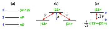
A simpler effective two-level system, shown in Fig. 4(c), with a reduced dipole-dipole matrix element can replace the three-level system of Fig. 4(b) in the theoretical calculations, because collective states and are equivalent and behave identically. We now denote state as state in the effective two-level system and the symmetric composite state + as state in Fig. 4(c). The other, antisymmetric composite state - is not considered, as it is unaffected by the operator of the dipole-dipole interaction and can be excluded from the analysis.
The most convenient form of equations for the density-matrix elements is the optical Bloch equations [27], where the complex exponents are excluded by a replacement of variables, and the detuning is present only in the expressions for the reduced coherences () and is absent in the expressions for the populations ():
| (3) |
Here, is the matrix element of the dipole-dipole interaction in circular frequency units. In Eqs. (3), we neglect the spontaneous and blackbody-radiation-induced depletion of the Rydberg states, as their effective lifetimes are tens of microseconds [28] and the related contribution to the Förster resonance width is just a few kilohertz, while in the experiments we typically observe Förster resonances of more than 1 MHz width.
In order to take into account the additional broadening phenomenologically, Eqs. (3) are modified using the method we have applied previously in Ref. [9] to account for the finite laser linewidths in a four-level theoretical model of the three-photon laser excitation of Rydberg states. In the equations for the coherences, we add the terms with /2 in order to introduce additional coherence decay. This method is called the phase-diffusion model and it describes the case where the driving radiation (or interaction) has random phase fluctuations but no amplitude fluctuations [29]. The validity of this model was grounded in Ref. [30]. Note that the noise spectrum in this model has a Lorentzian shape, which is not necessarily the case in the experiments.
The two-atom signal measured in our experiments is a fraction of Rydberg atoms in the final state 37S or a population of the final state 37S per atom, which is calculated for the interaction time t as
| (4) |
In order to find , Eqs. (3) can be solved analytically with the initial conditions . Their solution reduces to finding the roots of a cubic equation, if , , and are independent of time (see Appendix A). The resulting general analytical expressions are rather complicated, however, and in what follows we consider the analytical solutions only for some particular cases.
IV.2 Theory for the Förster resonance amplitude
The exact analytical solution of Eqs. (3) for the time evolution of the Förster resonance amplitude is given by
| (5) |
At the weak dipole-dipole interaction , Eq. (4) reduces to
| (6) |
The amplitude slowly goes to its steady-state value 1/4 as t increases. For the strong dipole-dipole interaction , the damped Rabi-like oscillations appear, while the steady-state value is also 1/4:
| (7) |
This is what can be observed with two Rydberg atoms, interacting in two spatially separated optical dipole traps, as in the experiments in Refs. [31,32]. At , the oscillations would never end, since there is no decoherence for the two motionless atoms considered here. But, in fact, cannot be zero as it is ultimately limited to a few kilohertz by the finite lifetimes of the Rydberg states [28].
In the realistic experiments, the atom positions are not fixed. The interaction term in Eqs. (6) and (7) has a fluctuating value that results in decoherence and washing out the Rabi-like oscillations in Eq.(7), even at . To calculate the resonance amplitude measured in our experiments, Eqs. (6) and (7) should be averaged over all possible spatial positions of the two interacting atoms in the excitation volume, which is formed by the two intersecting laser beams. In Ref. [22] we have shown that the averaging can be done using the nearest-neighbor probability distribution [33,34] with the average distance between nearest-neighbor atoms at volume density n0. Using this method, we find the approximate analytical solutions to the averaged amplitudes of Eqs. (6) and (7) (see Appendix B):
| (8) |
| (9) |
where
is the orientation-averaged reduced interaction matrix element at the average distance . Here, and are the dipole moments of transitions and . The fitting coefficients 0.44 and 0.55 have been found from the numerical simulations in the same way as in Ref. [22] for a cubic interaction volume (see Appendix B).
IV.3 Theory for the Förster resonance line shape
The analytical expressions for the line shape of the two-atom Förster resonances at are much more complicated than Eqs. (5)-(7). In the case when (weak interaction or short interaction time), the line shape for two frozen Rydberg atoms is approximately given by
| (10) |
Our numerical simulations have shown that this formula is quite precise (error less than 10%) for arbitrary , , , and t as far as . In fact, this is a general formula for the line shape of weak Förster resonances in two frozen Rydberg atoms. For the short interaction time , the line shape is given by just a Fourier transform of the short interaction pulse:
| (11) |
Its full width at half maximum (FWHM) in circular frequency units is . For the long interaction time , the line shape is given by a Lorentz profile with ,
| (12) |
In the opposite case of strong interaction , the line shape is approximately given by
| (13) |
This formula describes the saturation of the Förster resonance accompanied by the damped Rabi-like oscillations. As t or grow, there appears a flat-top contour with the width of the flat-top part , while the resonance wings are close to a Lorentzian. At , Eq. (13) gives independently of . This is because the steady-state solutions of Eqs. (3) are independent of if . For large , however, the time evolution is very slow, as described by the second term in Eq. (13).
If , the line shape is given by the undamped Rabi-like oscillations for arbitrary t,
| (14) |
The resonance width is either at or at .
The position-averaged line shape of the Förster resonance for two atoms in a single interaction volume can be obtained analytically only for Eqs. (13) or (14), because they correctly describe the saturation of resonances, otherwise the integral in the averaging diverges at short interaction distances. In Ref. [23], the averaging has been performed for the Lorentz pre-factor of Eq. (14) and an analytical formula has been obtained in terms of the standard sine and cosine integrals. This formula predicts a cusp-shaped Förster resonance at high Rydberg atom density, but it does not provide the time dependence of the amplitude and line shape.
In our averaging here, we use not the Lorentz pre-factor but Eq. (13) with , as discussed in Appendix C. The averaged line shape turns out to also be a cusp, which is approximately described by the following formula:
| (15) |
The fitting coefficients 0.44 and a have been obtained by comparing Eq. (15) with the numerical simulations of Eqs. (3) averaged over a cubic interaction volume for the Förster resonance Rb(37P)+Rb(37P)Rb(37S)+Rb(38S). At MHz, we have found that for MHz and ; for MHz and ; and for MHz and . In all intermediate cases, a should be varied to fit experimental or numerical data.
Equation (15) is thus a general formula that describes the cusped line shape of the Förster resonance for two Rydberg atoms randomly positioned in a single interaction volume. It is valid for a broad range of all parameters, and in addition it describes the time dynamics of the Förster resonance for the interaction times . In particular, it gives the same result as Eq. (8) for the averaged resonance amplitude, although Eq. (8) was derived for the weak dipole-dipole interaction, while Eq. (15) was derived from Eq. (13) describing the strong interaction. This can be explained by the fact that upon spatial averaging, the interactions between distant atoms are weak in most cases, as discussed in several other papers [17,21,23].
The formation of the cusp-shaped resonance upon spatial averaging can be understood from the fact that at zero detuning, the interaction is long range (resonant dipole-dipole) and it is effective even for the distant atoms, while for nonzero detuning the interaction is short range (van der Waals) and it is much weaker for the distant atoms [10]. Therefore, upon spatial averaging, the resonance wings are reduced stronger than the resonance center, and this finally results in the cusped line shape.
Equation (15) allows us also to calculate the FWHM of the cusped Förster resonance:
| (16) |
For the weak resonance , the width is . For the strong resonance the width is . We thus see that at the strong interaction, the line width depends on time and grows with t. This finding is quite unusual, because it is generally believed that at the strong interaction the line width is defined only by [17,21,23]. This is a specific feature of the spatial averaging in a disordered atom ensemble. It stems from the fact that upon spatial averaging the third term in Eq. (13) averages to nearly zero, while the second term remains significant at and fully defines the averaged line shape in Eq. (15).
The only drawback of Eq. (15) is that it is invalid for the short interaction times (), when the Fourier broadening dominates. The Fourier broadening is described by the third term in Eq. (13), which cannot be spatially averaged analytically with its time-dependent part, so numerical calculations are required. For the analytical estimates, the averaged Fourier broadening is described with a certain accuracy by Eqs. (10) or (11) if is replaced by .
We note that the above theoretical considerations are valid only for two interacting Rydberg atoms, when analytical solution of the density-matrix equation is possible. For the larger N numerical simulations should be used [22].
IV.4 Experimental Förster resonance line shapes
Figure 5 presents the line shapes of the Förster resonance Rb(37P)+Rb(37P)Rb(37S)+Rb(38S) recorded in our experiment for N=2 detected Rydberg atoms at various t . The interaction time t is set by the length of the square-shaped controlling electric-field pulse shown in Fig. 3(c).
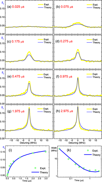
At the long interaction times (1.975 and 2.975 s), the resonance shape and width in Figs. 5(g) and 5(h) almost do not change with t . This means that the resonance takes its stationary form, and only its amplitude slowly grows with t according to Eq. (8). The resonance is cusp shaped, in agreement with Eq. (15). The observed small asymmetry in the red wing of the resonance is presumably due to some imperfection of the electric-field pulse in Fig. 3(c) because the electric field slightly varies during the pulse and its edges are not absolutely perfect.
The narrowest resonance appears at t=2.975 s. Its width in the electric-field scale is 16 mV/cm, corresponding to 1.9 MHz in the detuning scale. The detuning scale is obtained using the calculated polarizabilities of the collective Rydberg states in Fig. 1(c). Our attempts to obtain a narrower resonance by increasing t were not successful. Since the Fourier width of the interaction pulse is MHz and the estimated average interaction energy is MHz, they cannot be fully responsible for the 1.9 MHz resonance width. Therefore, there is an additional broadening MHz, apparently due to the unresolved hyperfine structure and parasitic ac electric fields. This observation agrees with what we have observed in our previous experiments [7,8].
The Fourier broadening of the resonances is demonstrated in Figs. 5(a)-5(e) at the shorter interaction times ( s). The Fourier width of the interaction pulse is significant at short t and the Förster resonance broadens according to Eq. (11), while its amplitude decreases.
In Figs. 5(a)-5(h), we also compare the experimental two-atom spectra at various t with the line shapes numerically calculated with Eqs. (3) and averaged over the random positions of two atoms in a cubic interaction volume. The fitting parameters in the theory were the volume size 262626 m3 and the additional broadening MHz. We also added a background signal that appears in the experiments due to parasitic transitions between Rydberg states induced by a 300 K blackbody radiation (BBR) [28]. These parameters allowed us to fit the time dependences of the experimental spectra, both for the amplitude [Fig. 5(i)] and width [Fig. 5(k)] of the two-atom Förster resonance. The amplitude and width are measured with respect to the BBR-induced background signal level.
The time dependence of the amplitude in Fig. 5(i) for s is also well fit by Eq. (8) at MHz and MHz. The time dependence of the width in Fig. 5(k) for s is mainly represented by the Fourier transform width . For s, the width becomes nearly constant and can be estimated with Eq. (16). For s, the width calculated with Eq. (16) is 1.46 MHz. If we add the Fourier width of 0.34, the total width of 1.8 MHz is close to the experimental width of 1.9 MHz.
One can conclude that our simple theoretical density-matrix model works well and provides correct analytical and numerical results for the time dynamics and cusped line shapes of the Förster resonances in two randomly positioned Rydberg atoms interacting in a single laser-excitation volume. Good agreement between experiment and theory confirms that any unresolved (hyperfine or Zeeman) structure or parasitic ac Stark broadening of the Förster resonances can be accounted for theoretically by a single parameter . This significantly reduces the number of equations and simplifies the calculations of the line shapes and time dynamics of the Förster resonances.
V Radio-frequency-assisted Förster resonances
As the rf-induced Förster resonances can be used to enhance the interactions between Rydberg atoms at long distances and to tune the van der Waals to resonant dipole-dipole interaction, we have performed the experiments where rf field of various frequencies and amplitudes was intentionally added. Our first experimental results were published in Ref. [10]. Here we analyze in more detail the main features of the rf-assisted Förster resonances and provide their comparison with theory.
V.1 Theory of rf-assisted Förster resonances
The physical interpretation of the rf-assisted Förster resonances was given in several papers [4,5,35,36]. A comprehensive theoretical analysis can be found in Ref. [36]. Several features should be emphasized.
First, the rf field induces single- and multi-photon transitions between collective states, as shown by the arrows in Fig. 6(a) for the ”accessible” Stark-tuned Förster resonance Rb(37P)+Rb(37P)Rb(37S)+Rb(38S) and in Fig. 6(b) for the ”inaccessible” Förster resonance Rb(39P)+Rb(39P)Rb(39S)+Rb(40S), which cannot be Stark-tuned by the dc electric field [10]. The rf photons of frequency compensate for the Förster energy defect when it has values that are multiples of , i.e., , with m being an integer. Multi-photon rf transitions can be driven if the rf field is strong enough. Similar Förster resonances between collective Rydberg states can also be induced by microwave fields [37].
Second, rf-assisted Förster resonances can also be explained in terms of the Floquet sidebands induced by a periodic perturbation of the Rydberg energy levels by the rf electric field due to the Stark effect [5,35,36]. Such sidebands were observed experimentally in the laser-excitation spectra of cold Rb Rydberg atoms and reported in our paper [10], as well as in several other experiments with Rydberg atoms in the vapor cells [38,39] and atomic beams [40,41]. Following Ref. [36], one should consider the Stark effect in a composite electric field consisting of dc and rf parts,
| (17) |
Then the time-dependent energy shift of a Rydberg level with nonzero quantum defect is
| (18) |
The term in the brackets is responsible for the ac Stark shift of the Rydberg level in the rf field [36]. The terms with and drive the transitions between collective states if .
The Floquet approach gives the eigenenergies of a Rydberg atom in a composite dc+rf field [36] as an infinite number of energy sidebands separated by [36]. For the Rydberg states experiencing quadratic Stark effect the relative amplitudes of the wave functions of the Floquet sidebands are described by the generalized Bessel functions,
| (19) |
while the wave function of the nL Rydberg state is
| (20) |
The rf-assisted Förster resonances arise for the Floquet sidebands that satisfy the resonance condition and intersect at some particular values of the dc electric field. Such resonances can also be observed when the rf-frequency is scanned and rf transitions of various orders are consequently induced [5]. At , the odd sidebands disappear according to Eq. (18) since only is nonzero, while the even sidebands are weak. Therefore, the rf-field alone hardly drives the transitions between collective states with a quadratic Stark effect, so a dc field should also be present.
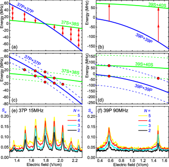
Figure 6(c) shows the energy levels of the initial 37P+37P and final 37S+38S collective states of two Rydberg atoms in electric field in the presence of the first-order Floquet sidebands at 15 MHz. Their intersections correspond to rf-assisted Förster resonances. These resonances are presented in Fig. 6(e) on the experimental record at a 200 mV rf-amplitude. This amplitude is high enough to induce the rf transitions of up to the fourth order. Multiple rf-assisted resonances are observed due to numerous intersections of the Floquet levels in Fig. 6(c). It is remarkable that the first- and second-order resonances have nearly the same amplitude as the central resonance. This indicates that the strength of the dipole-dipole interaction at the rf-assisted Förster resonances is comparable with that for ordinary Förster resonances without the rf field.
Figures 6(d) and 6(f) show the same for the Förster resonance on the 39P3/2 state at 90 MHz and 100 mV. A narrow second-order resonance at 1.49 V/cm is well seen along with a much stronger first-order resonance at 0.57 V/cm. The first-order resonance saturates and broadens with cusped line shape as N increases, while the second-order resonance is unsaturated and remains narrow for all N.
Third, the amplitudes and line shapes of the rf-assisted Förster resonances depend on many parameters (interaction energy, interaction time, orientation of dipole moments, number of atoms, dc and rf electric-field strengths) and should be calculated numerically using the density-matrix equations to compare them with experiment. In the adiabatic approximation the Förster resonance detuning in Eqs. (3) adiabatically follows the Stark shift in the oscillating composite electric field F given by Eq. (17):
| (21) |
V.2 Experimental results for rf-assisted Förster resonances
The left-hand column in Fig. 7 presents the experimental two-atom spectra of the Förster resonance in a 15 MHz rf field of various amplitudes at s. Without the rf field, a single peak at 1.79 V/cm is a ”true” Stark-tuned Förster resonance. Application of the rf field induces additional Förster resonances which are rf-assisted resonances of various orders. The frequency interval between the peaks corresponds to exactly 15 MHz, taking into account the calculated polarizabilities of these Rydberg states [10]. Increasing the amplitude of the rf field leads to the appearance of the higher-order resonances. At the maximum amplitude of 300 mV, even the fifth-order resonance can be seen.
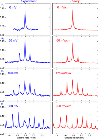
The right-hand column in Fig. 7 presents the spectra, which have been numerically calculated using Eqs. (3) and (21) and then spatially averaged. The fitting parameters in the theory were the volume size 303030 m3 and the additional broadening MHz. A BBR-induced background signal is added to the theoretical spectra. The theoretical spectra match the experimental ones very well, both in the number and amplitude of the observed sidebands and in the line shapes at various rf amplitudes.
However, in order to obtain this agreement, in the simulations we had to take the rf-field strength 17% larger than the one we measured in the experiments (the experimental rf amplitudes indicated in Fig. 7 should be divided by the 1 cm spacing between our electric-field plates). We also did not manage to calculate correctly the sideband amplitudes in Fig. 7 with Eqs. (19) and (20). This disagreement remains unclear and should be a subject of another dedicated study. One of the possible reasons can be the violation of the adiabatic approximation used in Eq. (21).
Another discrepancy in Fig. 7 is the central peak at 1.79 V/cm and 300-mV rf amplitude. While theory predicts that it should be narrow and small, in the experiment it appears rather broad. The reason is that in the experiment, this peak is formed due to two processes. As can be seen from the electric pulse shape in Fig. 3(d), the rf pulse is applied with 100 ns delay with respect to the leading edge of the electric pulse. During that delay, there is no rf field, so a normal Fourier-broadened Förster resonance similar to that in Fig. 5(b) should appear. Then the rf pulse is on and this resonance is formed in the rf field. At the large amplitude of 300 mV, this field causes the ac Stark shift of the Rydberg level in the rf field, as noted below Eq. (18). As a result, the central peak is formed by a broadened Förster resonance in a short dc field pulse and by a narrower shifted resonance in the rf field.
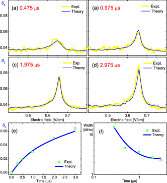
Now we will turn to the ”inaccessible” Förster resonance which cannot be tuned by the dc electric field. Its collective energy levels in the dc electric field are shown in Fig. 6(b). The dc field alone increases the energy detuning and makes the interaction between Rb(39P) atoms less efficient. However, as we have shown in Ref. [10], the rf field can induce transitions between collective states, so the population transfer at the Förster resonance occurs for the Floquet sidebands irrespective of the possibility to tune it by the dc field. In the present experiment, we applied rf field with 95 MHz frequency and 100 mV amplitude, which created the Floquet sidebands as in Fig. 6(d).
In Figs. 8(a)-8(d), we compare the experimental first-order rf-induced Förster resonances recorded for two atoms at various t to the theoretical line shapes numerically calculated with Eqs. (3) and (21) and averaged over random positions of two atoms in a cubic interaction volume. A BBR-induced background signal is added to the theoretical spectra. The fitting parameters in the theory were the volume size 161616 m3, the additional broadening MHz, and the rf-field strength 150 mV/cm (the latter is 50% larger than the experimentally measured one; this discrepancy remains unclear). These allowed us to fit the time dependences of the experimental spectra both for the amplitude [Fig. 8(e)] and width [Fig. 8(f)] of the two-atom Förster resonance. The amplitude and width are measured with respect to the BBR-induced background-signal level.
The narrowest resonance appears at t=2.975 s. It has a cusped shape, in agreement with Eq. (15), and its width in the electric-field scale is 18 mV/cm, corresponding to 1.1 MHz in the detuning scale, so this resonance is nearly two times narrower than that for the state. The detuning scale is obtained using the calculated polarizabilities of the collective Rydberg states in Fig. 1(d). The main contribution to thus comes from the parasitic ac electric fields. That is why in the theory we have to take MHz (i.e., two times larger than that for the state), and a smaller interaction volume to fit the amplitude of the two-atom resonances in Fig. 8.
RF-assisted inaccessible Förster resonances provide a way to tune the van der Waals to resonant dipole-dipole interactions and increase the interaction strength at long distances. This can be particularly useful for enhancing the dipole blockade effect [42,43] in mesoscopic Rydberg ensembles and for improving the fidelity of two-qubit quantum gates based on temporary Rydberg excitations [1,2] or of single-photon transistors based on the Förster resonances in Rydberg atoms [44]. For Rb nP3/2 states with n=40-100, the required rf-frequencies lie in the 100325 MHz range, and for nS states with n=70120, they are in the 140700 MHz range. These are reasonably low rf-frequencies, which can also be found in other alkali-metal atoms [45].
VI Conclusions
In this paper, we have performed a detailed experimental and theoretical analysis of the line shape and time dynamics of the Stark-tuned Förster resonances for two Rb Rydberg atoms interacting in a time-varying electric field.
In the theoretical analysis, we used an effective two-level density-matrix model that allowed us to account for the additional broadenings of the Förster resonances due to the unresolved hyperfine structure and parasitic ac electric fields. The analytical formulas have been obtained for the amplitude and line shape of the Förster resonances that correctly describe the time dynamics and dephasing of the Rabi-like population oscillations. Averaging over the random spatial positions of two Rydberg atoms in the interaction volume leads to the formation of a cusped line shape if the interaction time exceeds 1 s and the dipole-dipole interaction is strong enough to broaden the resonance. For the strong resonance, the line shape and width are shown to depend on the interaction time. At short interaction time, the resonance width is limited by the Fourier transform of the interaction pulse.
These theoretical considerations agree well with our experimental results for two Rb Rydberg atoms interacting in a single small laser-excitation volume. We have observed both the cusp-shaped Förster resonances at the long interaction time and Fourier broadened resonances at the short interaction time. The time dependences of their amplitude and width are well reproduced by the numerical simulations.
Good agreement between experiment and theory confirms that any unresolved (hyperfine or Zeeman) structure or parasitic ac Stark broadening of the Förster resonances can be accounted for theoretically by a single parameter . This significantly reduces the number of equations and simplifies the calculations of the line shapes and time dynamics of the Förster resonances. The time dynamics itself is represented either by the smooth exponential saturation in disordered atom ensembles, as observed in our present experiment, or by the damped Rabi-like oscillations for two frozen Rydberg atoms, as in Refs. [31,32].
In our experiments, we have also found that the transients at the edges of the controlling electric pulses strongly affect the line shapes of the Förster resonances, since the population transfer at the resonances occurs on a time scale of 100 ns, which is comparable with the duration of the transients. A short-term ringing at certain frequency causes additional radio-frequency-assisted Förster resonances, while non-sharp edges lead to an asymmetry.
An intentional application of the radio-frequency field induces transitions between collective states of two Rydberg atoms whose line shape depends on the interaction strengths and time. These resonances are the rf transitions between collective Floquet Rydberg states formed by the rf field due to the Stark effect. In the presence of the dc electric field, they can be induced both for Förster resonances which can be tuned by the dc field alone and for those which cannot be tuned. The van der Waals interaction of arbitrary Rydberg states can thus be efficiently tuned to resonant dipole-dipole interaction using the rf field.
Acknowledgements.
This work was supported by the RFBR Grants No. 14-02-00680 and No. 16-02-00383, the Russian Science Foundation Grant No. 16-12-00028 (for laser excitation of Rydberg states), the Siberian Branch of the Russian Academy of Sciences, the EU FP7-PEOPLE-2009-IRSES Project COLIMA, and the Novosibirsk State University.APPENDIX A. Analytical solution to the density-matrix equations
The density-matrix equations (3) can be solved analytically for arbitrary , , and , if these are independent of time. In order to do that, we first make the replacements
Then we substitute these into Eqs. (3) and obtain
After several substitutions we come to a single differential equation
Then we seek the solution as and obtain the cubic equation,
This equation has three roots, which are found analytically with the following sequence of equations taken from the mathematical handbooks:
Finally, the three roots are
Then we seek N in the form
with the initial conditions . These conditions give us the final exact analytical solution for the coefficients,
These formulas allow us to find N analytically and thus provide the exact analytical solution to Eqs. (3) for arbitrary , , , and t. The two-atom signal is then calculated as
The exact formulas are rather complex and cannot be presented in a clearly understandable way. Therefore, in Secs. IV B and IV C we consider the analytical solutions only for some particular cases where the formulas are reduced to short expressions.
APPENDIX B. Spatial averaging of the Förster resonance amplitude
For two interacting Rydberg atoms randomly positioned in a single laser-excitation volume, the spatial averaging of the Förster resonance amplitude given by Eqs. (6) or (7) can be performed analytically in the same way as in Ref. [22]. The averaging is done using the nearest-neighbor probability distribution [33,34] with the average distance between nearest-neighbor atoms at volume density n0,
The amplitude is averaged as
This integral is finite because Eqs. (6) and (7) are finite even at when . Its approximate analytical solution can be found if we use a conventional removal of the orientation-dependent part in Eq. (2); that is, we consider a ”scalar” dipole-dipole interaction. We remove the term in Eq. (2), so the interaction strength is now given by or . Its validity for disordered atom ensembles is grounded by the fact that mutual atom orientations are effectively averaged in such ensembles. Then we introduce
as the orientation-averaged reduced interaction matrix element at the average distance . Here, and are the dipole moments of transitions and . We also define a dimensionless integration variable .
At the weak dipole-dipole interaction, the integral to be found for the averaged amplitude of the Förster resonance is
The integrand in this expression is zero at and at , but it has a maximum at . This maximum is , while the width of the integrand in the x scale is of the order of 1. We therefore assumed that with a certain accuracy, the integral can be estimated as . Here are the fitting parameters, which can be found by numerical simulations. In fact, we should take to make the amplitude zero at t=0. Then our numerical simulation for a cubic interaction volume gave us , so the average amplitude for the weak interaction is approximately
At the strong dipole-dipole interaction, the integral to be found for the averaged amplitude of the Förster resonance is
In this case, we first do a trigonometric substitution and obtain a modified formula
An approximate analytical solution may be found as in Ref. [22] if we note that the main contribution to the integral comes from the very short distances, where the rapidly oscillating squared sine function can be replaced with its average value 1/2. Then the integration should start at and stop at some point , where , because the integrand exponentially drops at . Again, is a fitting parameter, which can be found by numerical simulations. Our simulations for a cubic interaction volume gave us , so the average amplitude for the strong interaction is approximately
APPENDIX C. Spatial averaging of the Förster resonance resonance line shape
The Förster resonance line shape can be averaged analytically in the same way as the amplitude. The main requirement is that the integral over R must not diverge at when . Therefore, the averaging can be done with Eqs. (13) or (14) that correctly describe the saturation of Förster resonances. But, in fact, Eq. (14) cannot be averaged analytically at due to its complicated dependence on R. Only its Lorentz pre-factor can be averaged as in Ref. [23], but it does not provide the dependence on the interaction time.
Therefore, in our averaging, we use Eq. (13) with . It is distinguished by the fact that upon spatial averaging, the third term in Eq. (13) averages to nearly zero at and , while the second term remains significant at and fully defines the averaged line shape. The averaged line shape to be found is
At large we can neglect in the denominators, and the integral reduces to
The integrand in this expression is zero at and at , but it has a maximum at . This maximum is , and the width of the integrand in the x scale is of the order of 1. We therefore suggested that, to some precision, the integral can be estimated as , with being the fitting parameters, which can be found by numerical simulations. In fact, we should take to make the amplitude zero at t=0. Then the average line shape for the weak interaction is approximately
Our numerical simulations have shown that this formula works well at large , but it does not work correctly near . We assumed that it can work better if we modify it phenomenologically as follows:
The fitting coefficients 0.44 and a have been obtained by comparing Eq. (15) to the numerical simulations of Eqs. (3) averaged over a cubic interaction volume for the Förster resonance Rb(37P)+Rb(37P)Rb(37S)+Rb(38S). Depending on , , and t, the values of a vary in the range from 2 to 4, as discussed in Sec. IV C.
References
- (1) M. Saffman, T. G. Walker, and K. Mlmer, Rev. Mod. Phys. 82, 2313 (2010).
- (2) I. I. Ryabtsev, I. I. Beterov, D. B. Tretyakov, V. M. Entin, and E. A. Yakshina, Physics Uspekhi 59, 196 (2016).
- (3) K. A. Safinya, J. F. Delpech, F. Gounand, W. Sandner, and T. F. Gallagher, Phys. Rev. Lett. 47, 405 (1981).
- (4) P. Pillet, D. Comparat, M. Muldrich, T. Vogt, N. Zahzam, V. M. Akulin, T. F. Gallagher, W. Li, P. Tanner, M. W. Noel, and I. Mourachko, in Decoherence, Entanglement and Information Protection in Complex Quantum Systems, edited by V. M. Akulin et al. (Springer, New York, 2005), p.411.
- (5) A. Tauschinsky, C. S. E. van Ditzhuijzen, L. D. Noordam, and H. B. van Linden van den Heuvell, Phys. Rev. A 78, 063409 (2008).
- (6) D. B. Tretyakov, I. I. Beterov, V. M. Entin, I. I. Ryabtsev, and P. L. Chapovsky, J. Exper. Theor. Phys. 108, 374 (2009).
- (7) I. I. Ryabtsev, D. B. Tretyakov, I. I. Beterov, and V. M. Entin, Phys. Rev. Lett. 104, 073003 (2010).
- (8) D. B. Tretyakov, I. I. Beterov, V. M. Entin, I. I. Ryabtsev, N. N. Bezuglov, and E. Arimondo, J. Exper. Theor. Phys. 114, 14 (2012).
- (9) V. M. Entin, E. A. Yakshina, D. B. Tretyakov, I. I. Beterov, and I. I. Ryabtsev, J. Exper. Theor. Phys. 116, 721 (2013).
- (10) D.B.Tretyakov, V.M.Entin, E.A.Yakshina, I.I.Beterov, C.Andreeva, and I.I.Ryabtsev, Phys. Rev. A 90, 041403(R) (2014).
- (11) I. I. Ryabtsev and I. M. Beterov, Phys. Rev. A 61, 063414 (2000).
- (12) I. I. Ryabtsev, D. B. Tretyakov, and I. I. Beterov, J. Phys. B 36, 297 (2003).
- (13) S. Westermann, T. Amthor, A. L. de Oliveira, J. Deiglmayr, M. Reetz-Lamour, and M. Weidemüller, Eur. Phys. J. D 40, 37 (2006).
- (14) J. Nipper, J. B. Balewski, A. T. Krupp, B. Butscher, R. Löw, and T. Pfau, Phys. Rev. Lett. 108, 113001 (2012).
- (15) P. J. Tanner, J. Han, E. S. Shuman, and T. F. Gallagher, Phys. Rev. Lett. 100, 043002 (2008).
- (16) K. C. Younge, A. Reinhard, T. Pohl, P. R. Berman, and G. Raithel, Phys. Rev. A 79, 043420 (2009).
- (17) J. R. Veale, W. Anderson, M. Gatzke, M. Renn, and T. F. Gallagher, Phys. Rev. A 54, 1430 (1996).
- (18) I. I. Ryabtsev, D. B. Tretyakov, I. I. Beterov, and V. M. Entin, Phys. Rev. A 76, 012722 (2007); Erratum: Phys. Rev. A 76, 049902(E) (2007).
- (19) W. R. Anderson, J. R. Veale, and T. F. Gallagher, Phys. Rev. Lett. 80, 249 (1998).
- (20) I. Mourachko, D. Comparat, F. de Tomasi, A. Fioretti, P. Nosbaum, V. M. Akulin, and P. Pillet, Phys. Rev. Lett. 80, 253 (1998).
- (21) B. Sun and F. Robicheaux, Phys. Rev. A 78, 040701(R) (2008).
- (22) I. I. Ryabtsev, D. B. Tretyakov, I. I. Beterov, V. M. Entin, and E. A. Yakshina, Phys. Rev. A 82, 053409 (2010).
- (23) B. G. Richards and R. R. Jones, Phys. Rev. A 93, 042505 (2016).
- (24) J. M. Kondo, D. Booth, L. F. Goncalves, J. P. Shaffer, and L. G. Marcassa, Phys. Rev. A 93, 012703 (2016).
- (25) B. Pelle, R. Faoro, J. Billy, E. Arimondo, P. Pillet, and P. Cheinet, Phys. Rev. A 93, 023417 (2016).
- (26) H. Park, T. F. Gallagher, and P. Pillet, Phys. Rev. A 93, 052501 (2016).
- (27) S. Stenholm, Foundations of Laser Spectroscopy (Dover, Mineoloa, NY, 2005).
- (28) I. I. Beterov, I. I. Ryabtsev, D. B. Tretyakov, and V. M. Entin, Phys. Rev. A 79, 052504 (2009).
- (29) G. S. Agarwal, Phys. Rev. Lett. 37, 1383 (1976).
- (30) K. Wodkiewicz, Phys. Rev. A 19, 1686 (1979).
- (31) S. Ravets, H. Labuhn, D. Barredo, L. Beguin, T. Lahaye, and A. Browaeys, Nature Physics 10, 914 (2014).
- (32) S. Ravets, H. Labuhn, D. Barredo, T. Lahaye, and A. Browaeys, Phys. Rev. A 92, 020701(R) (2015).
- (33) P. Hertz, Math. Ann. 67, 387 (1909).
- (34) S. Chandrasekhar, Rev. Mod. Phys. 15, 1 (1943).
- (35) P. Pillet, R. Kachru, N. H. Tran, W. W. Smith, and T. F. Gallagher, Phys. Rev. A 36, 1132 (1987).
- (36) C. S. E. van Ditzhuijzen, A. Tauschinsky, and H. B. van Linden van den Heuvell, Phys. Rev. A 80, 063407 (2009).
- (37) Y. Yu, H. Park, and T. F. Gallagher, Phys. Rev. Lett. 111, 173001 (2013).
- (38) M. G. Bason, M. Tanasittikosol, A. Sargsyan, A. K. Mohapatra, D. Sarkisyan, R. M. Potvliege, and C. S. Adams, New J. Phys. 12, 065015 (2010).
- (39) S. A. Miller, D. A. Anderson, and G. Raithel, New J. Phys. 18, 053017 (2016).
- (40) S. Yoshida, C. O. Reinhold, J. Burgdorfer, S. Ye, and F. B. Dunning, Phys. Rev. A 86, 043415 (2012).
- (41) V. Zhelyazkova and S. D. Hogan, Phys. Rev. A 92, 011402(R) (2015).
- (42) M. D. Lukin, M. Fleischhauer, R. Cote, L. M. Duan, D. Jaksch, J. I. Cirac, and P. Zoller, Phys. Rev. Lett. 87, 037901 (2001).
- (43) D. Comparat and P. Pillet, J. Opt. Soc. Am. B 27, A208 (2010).
- (44) D. Tiarks, S. Baur, K. Schneider, S. Dürr, and G. Rempe, Phys. Rev. Lett. 113, 053602 (2014).
- (45) J. H. Gurian, P. Cheinet, P. Huillery, A. Fioretti, J. Zhao, P. L. Gould, D. Comparat, and P. Pillet, Phys. Rev. Lett. 108, 023005 (2012).