The Moments of Lévy’s area using a sticky shuffle Hopf algebra

Abstract

Lévy’s stochastic area for planar Brownian motion is the difference of two iterated integrals of second rank against its component one-dimensional Brownian motions. Such iterated integrals can be multiplied using the sticky shuffle product determined by the underlying Itô algebra of stochastic differentials. We use combinatorial enumerations that arise from the distributive law in the corresponding Hopf algebra structure to evaluate the moments of Lévy’s area. These Lévy moments are well known to be given essentially by the Euler numbers. This has recently been confirmed in a novel combinatorial approach by Levin and Wildon. Our combinatorial calculations considerably simplify their approach.

Keywords: Lévy area; sticky shuffle algebras; Euler numbers.

MSC classifications: 60J65; 05A15.

1 Introduction

Lévy’s stochastic area is the signed area enclosed by the planar Brownian path and its chord. It was originally defined rigorously by Lévy [12] and now is intensively applied in several areas of modern mathematics, such as rough path analysis.

Let $B=\left(X,Y\right)$ be a planar Brownian motion in terms of components $X$ and $Y$ which are independent one-dimensional Brownian motions.

Definition 1

The Lévy area of $B$ over the time interval $[a,b)$ is the stochastic integral

$$\mathcal{A}_{[a,b)}=\dfrac{1}{2}\int_{a}^{b}\Bigl{(}\left(X-X(a)\right)dY-\left(Y-Y(a)\right)dX\Bigr{)}.$$

In this definition the integral takes the same value whether it is regarded as of Itô or Stratonovich type, but in the remainder of this paper all stochastic integrals will be of Itô type, in contrast to [11] where the Stratonovich integral is used.

Lévy studied the characteristic function in [12], [13], [14], [15] and [16]. He derived the following formula:

Theorem 2

(Lévy [12])

$$\mathbb{E}\!\left[\exp\left(iz\mathcal{A}_{[a,b)}\right)\right]\,=\,\operatorname{sech}\!\left(\tfrac{1}{2}\left(b-a\right)z\right).$$

We can expand the right-hand side of the formula in Theorem 2 using the Taylor series

$$\operatorname{sech}(z)\,=\,\sum_{m=0}^{\infty}\left(-1\right)^{m}\frac{A_{2m}}{\left(2m\right)!}z^{2m}\ ,$$ (1)

where the even Euler zigzag numbers $A_{2m}$ are related to the Riemann zeta function $\zeta$ by

$$\zeta\left(2m\right)\,=\,\frac{\pi^{2m}}{\left(2m\right)!}A_{2m}\,.$$ (2)

This expansion shows that the nonvanishing moments of the Lévy area $\mathcal{A}_{[a,b)}$ are given by

$$\mathbb{E}\!\left[\mathcal{A}_{[a,b)}\right]^{2m}\,=\,\,\left(\frac{b-a}{2}\right)^{\!2m}\!A_{2m}\,.$$ (3)

In [16], Lévy first showed Theorem 2 by using dyadic approximation. His second proof is based on the skew product representation of planar Brownian motion and depends on earlier work by Kac, Siegert, Cameron and Martin (see [16]). In 1980, Yor [20] simplified Lévy’s proof by employing a result on Bessel processes and an elementary result used by D.Williams. Shortly afterwards, Helmes and Schwane [5] revisited the problem by extending the $2$-dimensional set-up considered by Lévy to $d\geq 2$ dimensions. They considered the joint characteristic function of the stochastic process paired by the $d$-dimensional Brownian motion $W$ and a certain generalized Lévy area $\mathcal{A}_{[0,t]}^{J,x}$ given by

$$\mathcal{A}_{[0,t]}^{J,x}:=\int_{0}^{t}[W(s)+x(s)]J(s)dW(s).$$ (4)

Here, $[W(s)+x(s)]$ is viewed as a row-vector, a $1\times d$ matrix. For $d=2$, $x=0$ and $J=\bigl{[}\begin{smallmatrix}0&1\\ \!\!-1&0\end{smallmatrix}\bigr{]}$ the process $\mathcal{A}_{[0,t]}^{J,x}/2$ coincides with Lévy stochastic area $\mathcal{A}_{[0,t]}$ in Definition 1. Recently Levin and Wildon in [11] used iterated integrals and combinatorial arguments involving the shuffle product (see [6]) to prove Theorem 2. Our method starts from the same iterated integrals. Hence, we use that the integral in Definition 1 can be written as

$$\mathcal{A}_{[a,b)} = \dfrac{1}{2}\int_{a\,<x<\,y<\,b}\Bigl{(}dX(x)dY(y)-dY(x)dX(y)\Bigr{)}.$$ (5)

We may thus evaluate the moments as expectations of powers, using the so-called sticky shuffle [7] Hopf algebra. The multiplication in this algebra can be used to express the product of two iterated Itô stochastic integrals as a linear combination of such iterated integrals. Since the expectation of an iterated integral vanishes unless each of the individual integrators is time, the recovery formula [7, 1] involving higher order Hopf algebra coproducts reduces the evaluation of the moments to a combinatorial counting problem. Similar ideas were already used in [10] to calculate the moments in non-Fock quantum analogs of Lévy’s area.

The sticky shuffle Hopf algebra is reviewed in Section 2 and its use for reducing the evaluation of moments to a counting problem is described in Section 3. In Section 4, we apply combinatorial tools to show the main result. Finally, in the appendix, we provide a simple lemmas about Euler numbers needed in our calculations.

2 The sticky shuffle product Hopf algebra

Let there be given an associative algebra $\mathcal{L}$ over $\mathbb{C}$. The corresponding vector space $\mathcal{T}(\mathcal{L})$ of tensors of all ranks over $\mathcal{L}$ is defined as

$$\mathcal{T}(\mathcal{L})\,=\,\bigoplus\limits_{n=0}^{\infty}\bigotimes\limits_{j=1}^{n}\mathcal{L}\,.$$ (6)

We denote by $\left(\alpha_{0},\alpha_{1},\alpha_{2},...\right)$ the general element $\alpha=\alpha_{0}\oplus\alpha_{1}\oplus\alpha_{2}\oplus\cdots$ of $\mathcal{T}(\mathcal{L})$, where only finitely many of the $\alpha_{m}$ are nonzero. For each $\alpha_{m}\in$ $\bigotimes_{j=1}^{m}\mathcal{L}$ the corresponding embedded element $\left(0,0,...,\alpha_{m},0,...\right)$ of $\mathcal{T}(\mathcal{L})$ is denoted by $\left\{\alpha_{m}\right\}.$ In the following, we use the notational convention that, for arbitrary elements $\alpha$ of $\mathcal{T}(\mathcal{L})$ and $L$ of $\mathcal{L,}$ $\alpha\otimes L$ is the element of $\mathcal{T}(\mathcal{L})$ for which $\left(\alpha\otimes L\right)_{0}=0$ and $\left(\alpha\otimes L\right)_{n}=\alpha_{n-1}\otimes L$ for $n\geq 1.$

The so-called sticky shuffle product Hopf algebra over $\mathcal{L}$ is formed by equipping $\mathcal{T}(\mathcal{L})$ with the operations of product, unit, coproduct and counit defined as follows.

• The sticky shuffle product of arbitrary elements of $\mathcal{T}(\mathcal{L})$ is defined inductively by bilinear extension of the rules

  $$\{1_{\mathbb{C}}\}\left\{L_{1}\otimes L_{2}\otimes\cdots\otimes L_{m}\right\} = \left\{L_{1}\otimes L_{2}\otimes\cdots\otimes L_{m}\right\}\{1_{\mathbb{C}}\}$$ (7)

  $$= \left\{L_{1}\otimes L_{2}\otimes\cdots\otimes L_{m}\right\},$$

  $$\!\!\!\!\!\!\!\!\!\!\!\!\!\left\{L_{1}\otimes L_{2}\otimes\cdots\otimes L_{m}\right\}\left\{L_{m+1}\otimes L_{m+2}\otimes\cdots\otimes L_{m+n}\right\}$$

  $$= \left(\left\{L_{1}\otimes\cdots\otimes L_{m-1}\right\}\left\{L_{m+1}\otimes\cdots\otimes L_{m+n}\right\}\right)\otimes L_{m}$$

  $$+\left(\left\{L_{1}\otimes\cdots\otimes L_{m}\right\}\left\{L_{m+1}\otimes\cdots\otimes L_{m+n-1}\right\}\right)\otimes L_{m+n}$$

  $$+\left(\left\{L_{1}\otimes\cdots\otimes L_{m-1}\right\}\left\{L_{m+1}\otimes\cdots\otimes L_{m+n-1}\right\}\right)\otimes L_{m}L_{m+n}.$$

• The unit element for this product is $1_{\mathcal{T}(\mathcal{L})}=\left(1_{\mathbb{C}},0,0,...\right)$.

• The coproduct $\Delta$ is the map from $\mathcal{T}(\mathcal{L})$ to $\mathcal{T}(\mathcal{L})\otimes\mathcal{T}(\mathcal{L})$ defined by linear extension of the rules that $\Delta\left(1_{\mathcal{T}(\mathcal{L})}\right)=1_{\mathcal{T}(\mathcal{L})}\otimes 1_{\mathcal{T}(\mathcal{L})}=1_{\mathcal{T}(\mathcal{L})\otimes\mathcal{T}(\mathcal{L})}$ and

  $$\!\!\!\!\!\!\!\!\!\!\!\!\!\Delta\left\{L_{1}\otimes L_{2}\otimes\cdots\otimes L_{m}\right\}$$

  $$= 1_{\mathcal{T}(\mathcal{L})}\otimes\left\{L_{1}\otimes L_{2}\otimes\cdots\otimes L_{m}\right\}$$

  $$+\sum\limits_{j=2}^{m}\left\{L_{1}\otimes L_{2}\otimes\cdots\otimes L_{j-1}\right\}\otimes\left\{L_{j}\otimes L_{j+1}\otimes\cdots\otimes L_{m}\right\}$$

  $$+\left\{L_{1}\otimes L_{2}\otimes\cdots\otimes L_{m}\right\}\otimes 1_{\mathcal{T}(\mathcal{L})}.$$

• The counit $\varepsilon$ is the map from $\mathcal{T}(\mathcal{L})$ to $\mathbb{C}$ defined by linear extension of

  $$\varepsilon\left(1_{\mathcal{T}(\mathcal{L})}\right)=1_{\mathbb{C}}\ \text{ and }\ \varepsilon\left\{L_{1}\otimes L_{2}\otimes\cdots\otimes L_{m}\right\}=0\ \text{ for }\ m>0.$$ (10)

Remark 3

There is a useful alternative equivalent definition of the sticky shuffle product. We can define the product $\gamma=\alpha\beta$ by

$$\gamma_{N}\,=\sum_{A\cup B=\{1,2,...,N\}}\alpha_{\left|A\right|}^{A}\beta_{\left|B\right|}^{B}.$$ (11)

Here the sum is now over the $3^{N}$ not necessarily disjoint ordered pairs $(A,B)$ whose union is $\{1,2,...,N\}$, and the notation is as follows; $\left|A\right|$ denotes the number of elements in the set $A$ so that $\alpha_{\left|A\right|}$ denotes the homogeneous component of rank $\left|A\right|$ of the tensor $\alpha=\left(\alpha_{0},\alpha_{1},\alpha_{2},...\right),$ and $\alpha_{\left|A\right|}^{A}$ indicates that this component is to be regarded as occupying only those $\left|A\right|$ copies of $\mathcal{L}$ within $\bigotimes_{j=1}^{N}\mathcal{L}$ labelled by elements of the subset $A$ of $\{1,2,...,N\}.$ Thus with $\beta_{\left|B\right|}^{B}$ defined analogously the combination $\alpha_{\left|A\right|}^{A}\beta_{\left|B\right|}^{B}$ is a well-defined element of $\bigotimes_{j=1}^{N}\mathcal{L}$. Here, if $A\cap B\neq\emptyset$, double occupancy of a copy of $\mathcal{L}$ within $\bigotimes_{j=1}^{n}\mathcal{L}$ is reduced to single occupancy by using the multiplication in the algebra $\mathcal{L}$ as a map from $\mathcal{L\times L}$ to $\mathcal{L.}$ That (11) is equivalent to (• ‣ 2) is seen by noting that the three terms on the right-hand side of (• ‣ 2) correspond to the three mutually exclusive and exhaustive possibilities that $N\in A\cap B^{c},$ $N\in A^{c}\cap B$ and $N\in A\cap B$ in (11).

The recovery formula [1] expresses the homogeneous components of an element $\alpha$ of $\mathcal{T}(\mathcal{L})$ in terms of the iterated coproduct $\Delta^{(N)}\alpha$ by

$$\alpha_{N}=\left(\Delta^{(N)}\alpha\right)_{(1,1,...,\overset{(N)}{1})}.$$ (12)

Here, $\Delta^{(N)}$ is defined recursively by

$$\Delta^{(2)}=\Delta\quad\text{and}\quad\Delta^{(N)}=\left(\Delta\otimes\mbox{Id}_{\otimes^{(N-2)}\left(\mathcal{T}\left(\mathcal{L}\right)\right)}\right)\circ\Delta^{(N-1)}\quad\text{for}\quad N>2\,.$$ (13)

Hence, it is a map from $\mathcal{T}(\mathcal{L})$ to the $N$th tensor power

$$\bigotimes\!^{(N)}\mathcal{T}(\mathcal{L})\,=\,\bigotimes\!^{(N)}\bigoplus\limits_{n=0}^{\infty}\ \bigotimes\limits_{j=1}^{n}\mathcal{L}\,=\bigoplus\limits_{n_{1},n_{2},...,n_{N}=0}^{\infty}\ \bigotimes_{r=1}^{N}\ \bigotimes\limits_{j_{r}=1}^{n_{r}}\mathcal{L}$$ (14)

so that $\Delta^{(N)}\alpha$ has multirank components $\alpha_{\left(n_{1},n_{2},...,n_{N}\right)}$ of all orders. The recovery formula (12) also holds when $N=0$ and $N=1$ if we define $\Delta^{(0)}$ and $\Delta^{(1)}$ to be the counit $\varepsilon$ and the identity map $1_{\mathcal{T}(\mathcal{L})}$ respectively.

Note that $\Delta$ is multiplicative, $\Delta\left(\alpha\beta\right)=\Delta\left(\alpha\right)\Delta\left(\beta\right)$, where the product on the tensor square $\mathcal{T}(\mathcal{L})\otimes\mathcal{T}(\mathcal{L})$ is defined by linear extension of the rule

$$(a\otimes a^{\prime})(b\otimes b^{\prime})\,=\,ab\otimes a^{\prime}b^{\prime}\,.$$ (15)

3 Moments and sticky shuffles

We now describe the connection between sticky shuffle products and iterated stochastic integrals. We begin with the well-known fact that, for the one-dimensional Brownian motion $X$ and for $a\leq b,$

$$\left(X(b)-X(a\right))^{2}\,=\,2\!\int_{a\leq x<b}\!\!\!\!\!\!\!\!\left(X(x)-X(a)\right)dX(x)\ +\,\int_{a\leq x<b}\!\!\!\!\!\!\!\!dT(x),$$ (16)

where $T(x)=x$ is time. We introduce the Itô algebra $\mathcal{L=}\mathbb{C}\left\langle dX,dT\right\rangle$ of complex linear combinations of the basic differentials $dX$ and $dT,$ which are multiplied according to the table

$$\begin{tabular}[]{c|c}&$\begin{array}[]{cc}dX&dT\end{array}$\\ \hline\cr$\begin{array}[]{c}dX\\ dT\end{array}$&$\begin{array}[]{cc}dT&0\\ 0&0\end{array}$\end{tabular},$$ (17)

together with the corresponding sticky shuffle Hopf algebra $\mathcal{T}(\mathcal{L}).$ For each pair of real numbers $a<b,$ we introduce a map $J_{a}^{b}$ from $\mathcal{T}(\mathcal{L})$ to complex-valued random variables on the probability space of the Brownian motion $X$ by linear extension of the rule that, for arbitrary $dL_{1},dL_{2},\cdots dL_{m}\in\left\{dX,dT\right\}$

$$\!\!\!\!\!\!\!\!\!\!\!\!\!\!J_{a}^{b}\left\{dL_{1}\otimes dL_{2}\otimes\dotsm\otimes dL_{m}\right\}$$

$$= \!\!\!\!\int_{a\leq x_{1}<x_{2}<\dotsb<x_{m}<b}dL_{1}(x_{1})\,dL_{2}(x_{2})\,dL_{3}(x_{3})\dotsm\,dL_{m}(x_{m})$$

$$= \!\!\!\!\int_{a}^{b}\!\!\dotsm\int_{a}^{x_{4}}\!\!\int_{a}^{x_{3}}\!\!\int_{a}^{x_{2}}\!\!dL_{1}(x_{1})\,dL_{2}(x_{2})\,dL_{3}(x_{3})\dotsm\,dL_{m}(x_{m}).$$

By convention $J_{a}^{b}$ maps the unit element of the algebra $\mathcal{T}(\mathcal{L})$ to the unit random variable identically equal to 1.

Then (16) can be restated as follows,

$$J_{a}^{b}\left(\left\{dX\right\}\right)J_{a}^{b}\left(\left\{dX\right\}\right)=J_{a}^{b}\left(\left\{dX\right\}\left\{dX\right\}\right),$$ (19)

using the fact that $\left\{dX\right\}^{2}=2\left\{dX\otimes dX\right\}+\left\{dT\right\}.$

The following more general Theorem is probably known to many probabilists.

Theorem 4

For arbitrary $\alpha$ and $\beta$ in $\mathcal{T}(\mathcal{L})$,

$$J_{a}^{b}(\alpha)J_{a}^{b}(\beta)=J_{a}^{b}(\alpha\beta)\,.$$

Proof. By bilinearity it is sufficient to consider the case when

$$\alpha=\left\{dL_{1}\otimes dL_{2}\otimes\cdots\otimes dL_{m}\right\},\ \beta=\left\{dL_{m+1}\otimes dL_{m+2}\otimes\cdots\otimes dL_{m+n}\right\}$$ (20)

for $dL_{1},dL_{2},\cdots,dL_{m+n}\in\left\{dX,dT\right\}.$ In this case Theorem 4 follows, using the inductive definition (• ‣ 2) for the sticky shuffle product, from the product form of Itô’s formula,

$$d\left(\xi\eta\right)=\left(d\xi\right)\eta+\xi d\eta+\left(d\xi\right)d\eta$$ (21)

where stochastic differentials of the form $d\xi=FdX+GdT,$ with stochastically integrable processes $F$ and $G$, are multiplied using the table (17).

 

For planar Brownian motion $B=\left(X,Y\right)$ the Ito table (17) becomes

$$\begin{tabular}[]{c|c}&$\begin{array}[]{cc}\begin{array}[]{cc}dX&dY\end{array}&dT\end{array}$\\ \hline\cr$\begin{array}[]{c}\begin{array}[]{c}dX\\ dY\end{array}\\ dT\end{array}$&$\begin{array}[]{cc}\begin{array}[]{cc}dT&0\\ 0&dT\end{array}&\begin{array}[]{c}0\\ 0\end{array}\\ \begin{array}[]{cc}0&0\end{array}&0\end{array}$\end{tabular}.$$ (22)

Corollary 5

Theorem 4 holds when $\mathcal{L}$ is the algebra defined by the multiplication table (22).

Basic for our calculations is the next theorem. It follows from the fact that expectations of stochastic integrals against either $dX$ or $dY$ as integrators are zero.

Theorem 6

For arbitrary $n\in\mathbb{N,}$ $a<b\in\mathbb{R}$ and basis elements $dL_{1}$, $dL_{2}$, …, $dL_{n}\in\{dX,dY,dT\}$,

$$\mathbb{E}\!\left[J_{a}^{b}\left\{dL_{1}\otimes dL_{2}\otimes...\otimes dL_{n}\right\}\right]\,=\,0$$

unless

$$dL_{1}=dL_{2}=\cdots=dL_{n}=dT.$$

In view of (5)

$$\mathcal{A}_{[a,b)}\,=\,\dfrac{1}{2}J_{a}^{b}(dX\otimes dY-dY\otimes dX)\,.$$ (23)

Now consider the moments sequence of classical Lévy area in terms of the basis $\left(dX,dY,dT\right)$, i.e., Eqn. (23). In view of Theorem 4

$$\left[\mathcal{A}_{[a,b)}\right]^{n} = {\dfrac{1}{2^{n}}}\left(J_{a}^{b}(dX\otimes dY-dY\otimes dX)\right)^{n}$$ (24)

$$= {\dfrac{1}{2^{n}}}J_{a}^{b}\left(\{dX\otimes dY-dY\otimes dX\}^{n}\right)$$

The $n$th sticky shuffle power $\left\{dX\otimes dY-dY\otimes dX\right\}^{n}$ will consist of non-sticky shuffle products of rank $2n$ together with terms of lower ranks $n,n+1,...,2n-1$, all of which except the rank $n$ term will contain one or more copies of $dX$ and $dY$, and will thus not contribute to the expectation in view of Theorem 6. The term of rank $n$ will be a multiple of $dT\otimes dT\cdots\otimes\overset{(n)}{dT}.$ Thus we can write

$$\left\{dX\otimes dY-dY\otimes dX\right\}^{n}\,=\,w_{n}\bigl{\{}dT\otimes dT\cdots\otimes\overset{(n)}{dT}\bigr{\}}+\,\text{terms of rank}>n.$$ (25)

for some coefficient $w_{n}$. The corresponding moment is given by

$$\mathbb{E}\!\left[\mathcal{A}_{[a,b)}\right]^{n} = \dfrac{w_{n}}{2^{n}}\,\mathbb{E}\!\left[J_{a}^{b}\bigl{(}\{dT\otimes dT\cdots\otimes\overset{(n)}{dT}\}\bigr{)}\right]$$ (26)

$$= \dfrac{w_{n}}{2^{n}}\int_{a\leq x_{1}<x_{2}<\cdots<x_{n}<b}dx_{1}\,dx_{2}\dotsm\,dx_{n}$$

$$= \dfrac{w_{n}\left(b-a\right)^{n}}{2^{n}n!}.$$

By the recovery formula (12) and the multiplicativity of the $n$th order coproduct $\Delta^{\left(n\right)},$

$$\!\!\!\!\!\!\!\!\!\!\!\!w_{n}dT\otimes dT\cdots\otimes\overset{(n)}{dT}$$ (27)

$$= \left\{\left\{dX\otimes dY-dY\otimes dX\right\}^{n}\right\}_{n}$$

$$= \left(\Delta^{(n)}\bigl{(}\left\{dX\otimes dY-dY\otimes dX\right\}^{n}\bigr{)}\right)_{\!\!(1,1,...,\overset{\left(n\right)}{1})}$$

$$= \left(\Bigl{(}\Delta^{(n)}\bigl{(}\left\{dX\otimes dY-dY\otimes dX\right\}\bigr{)}\Bigr{)}^{n}\right)_{\!\!(1,1,...,\overset{\left(n\right)}{1})}.$$

Now

$$\!\!\!\!\!\!\!\!\!\!\!\!\Delta^{(n)}\bigl{(}\left\{dX\otimes dY-dY\otimes dX\right\}\bigr{)}$$ (28)

$$= \sum_{1\leq j\leq n}1_{\mathcal{T}(\mathcal{L})}\otimes\cdots\otimes\overset{(j)}{\left\{dX\otimes dY-dY\otimes dX\right\}}\otimes\cdots\otimes 1_{\mathcal{T}(\mathcal{L})}$$

$$+\sum_{1\leq j\,<k\leq n}\biggl{(}1_{\mathcal{T}(\mathcal{L})}\otimes\cdots\otimes\overset{\left(j\right)}{\left\{dX\right\}}\otimes\cdots\otimes\overset{\left(k\right)}{\left\{dY\right\}}\otimes\cdots\otimes\overset{\left(n\right)}{1_{\mathcal{T}(\mathcal{L})}}$$

$$-\ 1_{\mathcal{T}(\mathcal{L})}\otimes\cdots\otimes\overset{\left(j\right)}{\left\{dY\right\}}\otimes\cdots\otimes\overset{\left(k\right)}{\left\{d{X}\right\}}\otimes\cdots\otimes\overset{\left(n\right)}{1_{\mathcal{T}(\mathcal{L})}}\biggr{)}$$

The first term of this sum, being of rank $2,$ cannot contribute to the component of joint rank $(1,1,...,\overset{\left(n\right)}{1})$ of the $n$th power of $\Delta^{(n)}\left(\left\{dX\otimes dY-dY\otimes dX\right\}\right)$, where product in the nth tensor power $\bigotimes\!^{(N)}\mathcal{T}(\mathcal{L})$ is defined exactly as in the case $n=2$ in (15). Thus

$$\!\!\!\!\!\!\!\!\!\!\!\!w_{n}dT\otimes dT\cdots\otimes\overset{(n)}{dT}$$

$$= \left(\left(\Delta^{(n)}\bigl{(}\left\{dX\otimes dY-dY\otimes dX\right\}\bigr{)}\right)^{\!n\,}\right)_{\!\!(1,1,...,\overset{\left(n\right)}{1})}$$

$$= \left(\left(\sum_{1\leq j\,<k\leq n}\biggl{(}1_{\mathcal{T}(\mathcal{L})}\otimes\cdots\otimes\overset{(j)}{\left\{dX\right\}}\otimes\cdots\otimes\overset{(k)}{\left\{dY\right\}}\otimes\cdots\otimes\overset{(n)}{1_{\mathcal{T}(\mathcal{L})}}\biggr{.}\right.\right.$$

$$\left.\left.\biggl{.}-\ 1_{\mathcal{T}(\mathcal{L})}\otimes\cdots\otimes\overset{(j)}{\left\{dY\right\}}\otimes\cdots\otimes\overset{(k)}{\left\{dX\right\}}\otimes\cdots\otimes\overset{(n)}{1_{\mathcal{T}(\mathcal{L})}}\biggr{)}\right)^{\!\!\!n\,}\right)_{\!\!\!(1,1,...,\overset{\left(n\right)}{1})}$$

This calculation of $w_{n}$ can be finished using some combinatorics. We do that in the following section.

4 The moments of Lévy’s area

To evaluate the moments $\mathbb{E}\!\left[\mathcal{A}_{[a,b)}\right]^{n}$​, we need to calculate the number $w_{n}$, as explained in (26). By (3), we have

$$w_{n}\,dT\otimes dT\cdots\otimes\overset{(n)}{dT}\,\,=\,\left(\left(\sum_{h\neq k}\operatorname{sn}(h,k)R_{h,k}\right)^{\!\!\!n\,}\right)_{\!\!\!(1,1,...,\overset{\left(n\right)}{1})}$$ (30)

with

$$R_{h,k}\,:=\,1\otimes\dots\otimes 1\otimes\overset{(h)}{\{dX\}}\otimes 1\otimes\dots\otimes 1\otimes\overset{(k)}{\{dY\}}\otimes 1\otimes\dots\otimes 1$$ (31)

and

$$\operatorname{sn}(h,k)\,:=\,\begin{cases}+1&\text{if $h<k$},\\ -1&\text{if $h>k$}.\end{cases}$$ (32)

The $n$th power in (30) is based on the sticky shuffle product in $\mathcal{T}(\mathcal{L})$ and its extension to the nth tensor power $\bigotimes\!^{(n)}\mathcal{T}(\mathcal{L})$, as described in (15) for $n=2$.

If we set $e:=(h,k)$, then we may also write $R_{e}$ for $R_{h,k}$ and $\operatorname{sn}(e)$ for $\operatorname{sn}(h,k)$. Using distributivity, this yields

$$w_{n}\,dT\otimes dT\cdots\otimes\overset{(n)}{dT}\,=\,\sum\ \left(\prod_{\ell=1}^{n}\operatorname{sn}(e_{\ell})\right)\!\!\left(\prod_{\ell=1}^{n}R_{e_{\ell}}\right)_{\!\!\!(1,1,...,\overset{\left(n\right)}{1})}\,,$$ (33)

where the sum runs over all $n$-tuples $(e_{1},e_{2},\dotsc,e_{n})$ of pairs $(h,k)$ with $h\neq k$. We may imagine each pair $e_{\ell}=(h_{\ell},k_{\ell})$ as a directed edge, an arc, from $h_{\ell}$ to $k_{\ell}$. Each $n$-tuples $(e_{1},e_{2},\dotsc,e_{n})$ is then a directed labeled multigraph, we say a digraph, on the vertex set $V:=\{1,2,\dotsc,n\}$. We have to see what the individual arcs $e_{\ell}$ of a digraph $(e_{1},e_{2},\dotsc,e_{n})$ contribute to its corresponding summand $\pm\prod_{\ell=1}^{n}R_{e_{\ell}}$ inside the sum (33). For example, in the case $n=4$, the two arcs $e_{1}=(1,2)$ and $e_{2}=(3,2)$ contribute

$$\begin{split}\operatorname{sn}(e_{1})&\operatorname{sn}(e_{2})\bigl{(}R_{e_{1}}R_{e_{2}}\bigr{)}_{\!(1,1,1,1)}\\ &\,=\,-\bigl{(}(\{dX\}\otimes\{dY\}\otimes 1\otimes 1)(1\otimes\{dY\}\otimes\{dX\}\otimes 1)\bigr{)}_{\!(1,1,1,1)}\\ &\,=\,-\bigl{(}\{dX\}1\bigr{)}_{\!(1)}\otimes\bigl{(}\{dY\}\{dY\}\bigr{)}_{\!(1)}\otimes\bigl{(}1\{dX\}\bigr{)}_{\!(1)}\otimes\bigl{(}1\cdot 1\bigr{)}_{\!(1)}\\ &\,=\,-\,dX\otimes dT\otimes dX\otimes 1\,,\end{split}$$ (34)

where we basically ignored $e_{3}$ and $e_{4}$ (and the corresponding $R_{e_{3}}$, $R_{e_{4}}$, $\operatorname{sn}(e_{3})$ and $\operatorname{sn}(e_{4})$) to illustrate how the product operates.

In order to calculate the coefficient $w_{n}$ of $dT\otimes dT\otimes\dotsm\otimes dT$ in (33), we need to retain only those summands $\pm\prod_{\ell=1}^{n}R_{e_{\ell}}$ that contribute a scalar multiple of $dT\otimes dT\otimes\dotsm\otimes dT$. We may discard other summands. Hence, we do not have to sum over all digraphs $(e_{1},e_{2},\dotsc,e_{n})$. To see which ones we have to retain, let us assume that $(e_{1},e_{2},\dotsc,e_{n})$ yields a multiple of $dT\otimes dT\otimes\dotsm\otimes dT$ in (33). Since the $n$ copies of $dX$ and $n$ copies of $dY$ in the unexpanded product $\prod_{\ell=1}^{n}R_{e_{\ell}}$ must yield $n$ copies of $dT$​, one in each possible position, each vertex of the digraph $(e_{1},e_{2},\dotsc,e_{n})$ must have either exactly two incoming and no outgoing arcs (corresponding to a $(dY)^{2}$ ) or exactly two outgoing and no incoming arcs (corresponding to a $(dX)^{2}$ ). This shows that, inevitable, $(e_{1},e_{2},\dotsc,e_{n})$ must consist of disjoint alternatingly oriented cycles that cover $V$​, cycles whose arcs go “forward - backward - forward - backward - …”. Every such digraph $(e_{1},e_{2},\dotsc,e_{n})$ has necessarily an even number of vertices, $n=2m$, and contributes either $+1$ or $-1$ to $w_{2m}$. In particular, this means that for odd $n$ we do not obtain any term $dT\otimes dT\otimes\dotsm\otimes dT$ in (33), i.e. $w_{n}=0$ for odd $n$.

Before we do the counting in the case $n=2m$, we transform the alternatingly oriented labeled digraphs $(e_{1},e_{2},\dotsc,e_{2m})$ into cyclically oriented digraphs $D$, and, eventually, into permutations of a certain kind. Turning around each second arc in each cycle, we get cyclicly oriented cycles (like cyclic one way roads). These disjoint cycles still cover $V$ and have even length, as they arose from alternatingly oriented cycles. Conversely, we can always go back to alternatingly oriented cycles by flipping each second arc. To be precise, each (labeled) even cycle has two alternating orientations but also two cyclic orientations. Hence, there are several ways to match our labeled alternatingly oriented digraphs $(e_{1},e_{2},\dotsc,e_{2m})$ and the new cyclically oriented digraphs. However, they are all valid. We only need to know that there exist a bijection, a bijection under which every image differs from its pre-image $(e_{1},e_{2},\dotsc,e_{2m})$ in exactly $m$ edges. This will then result in an additional factor of $(-1)^{m}$ in our calculations. Moreover, at this point, our cyclically oriented digraphs do not contain multiple arcs, so that we may forget the labels $1,2,\dotsc,2m$ of the arcs $e_{1},e_{2},\dotsc,e_{2m}$. If a digraph $D$ with $2m$ many unlabeled arcs has no multiple (no indistinguishable) arcs, then it corresponds to exactly $(2m)!$ many labeled digraphs, yielding a factor of $(2m)!$ in our sum. Very careful readers might be astonished that we could not drop the edge labels earlier in this way. We invite them to investigate the case $m=1$ to see why.

Eventually, we can now turn towards permutations in the symmetric group $\mathcal{S}_{2m}$ as representatives for the diagraphs $D$ and the corresponding summands $\pm\prod_{\ell=1}^{n}R_{e_{\ell}}$ inside the sum of (33). We may view each arc $(h,k)$ in any cyclically oriented unlabeled digraph $D$ as the assignment of a function value, $h\mapsto k=:\operatorname{\mathfrak{s}}(h)$, and obtain a permutation $\operatorname{\mathfrak{s}}=\operatorname{\mathfrak{s}}_{D}$ on $V=\{1,2,\dotsc,2m\}$. In our case, the cycles of $\operatorname{\mathfrak{s}}$ have even length. We denote with $\mathcal{D}_{2m}\subseteq\mathcal{S}_{2m}$ the set of all permutations of this kind. Putting all this together, and keeping track of the signs, we see that

$$w_{2m}\,=\,(-1)^{m}(2m)!\sum_{\operatorname{\mathfrak{s}}\in\mathcal{D}_{2m}}\operatorname{sn}(\operatorname{\mathfrak{s}})\,,$$ (35)

where

$$\operatorname{sn}(\operatorname{\mathfrak{s}})\,:=\,\prod_{j=1}^{2m}\operatorname{sn}(j,\operatorname{\mathfrak{s}}(j))\,.$$ (36)

To determine this sum, we cancel off some summands $\operatorname{\mathfrak{s}}$ with opposite signs $\operatorname{sn}(\operatorname{\mathfrak{s}})$. We call a point $h\in V$ a transit of $\operatorname{\mathfrak{s}}$ if

$$\text{either}\quad\operatorname{\mathfrak{s}}^{-1}(h)<h<\operatorname{\mathfrak{s}}(h)\quad\text{or}\quad\operatorname{\mathfrak{s}}^{-1}(h)>h>\operatorname{\mathfrak{s}}(h)\ .$$ (37)

Let $\mathcal{D}_{2m}^{\prime}$ bet the set of all $\operatorname{\mathfrak{s}}\in\mathcal{D}_{2m}$ which have at least one transit. We show that the elements of $\mathcal{D}_{2m}^{\prime}$ cancel out completely and can be ignored in our sum. Obviously, every $\operatorname{\mathfrak{s}}\in\mathcal{D}_{2m}^{\prime}$ contains a unique smallest transit $h$, and we obtain a permutation $\operatorname{\mathfrak{s}}^{\prime}$ of $V\!\setminus\!\{h\}$ by replacing the chain of assignments $\operatorname{\mathfrak{s}}^{-1}(h)\mapsto h\mapsto\operatorname{\mathfrak{s}}(h)$ with the shorter chain $\operatorname{\mathfrak{s}}^{-1}(h)\longmapsto\operatorname{\mathfrak{s}}(h)$. The new permutation $\operatorname{\mathfrak{s}}^{\prime}$ has a unique odd cycle

$$j_{1}\mapsto j_{2}\mapsto\dotsb\mapsto\operatorname{\mathfrak{s}}^{-1}(h)\longmapsto\operatorname{\mathfrak{s}}(h)\mapsto\dotsm\mapsto j_{2k-1}\mapsto j_{1}.$$ (38)

If we walk once around this cycle and observe the indices $j_{1},j_{2},j_{3},\dotsc$ as a kind of altitude, then we will cross the altitude $h$ as many times upwards, from below $h$ to above $h$, as downwards, from above $h$ to below $h$. Hence, there is an even number of ways to reinsert $h$ as transit into that odd cycle, see Fig. 1.

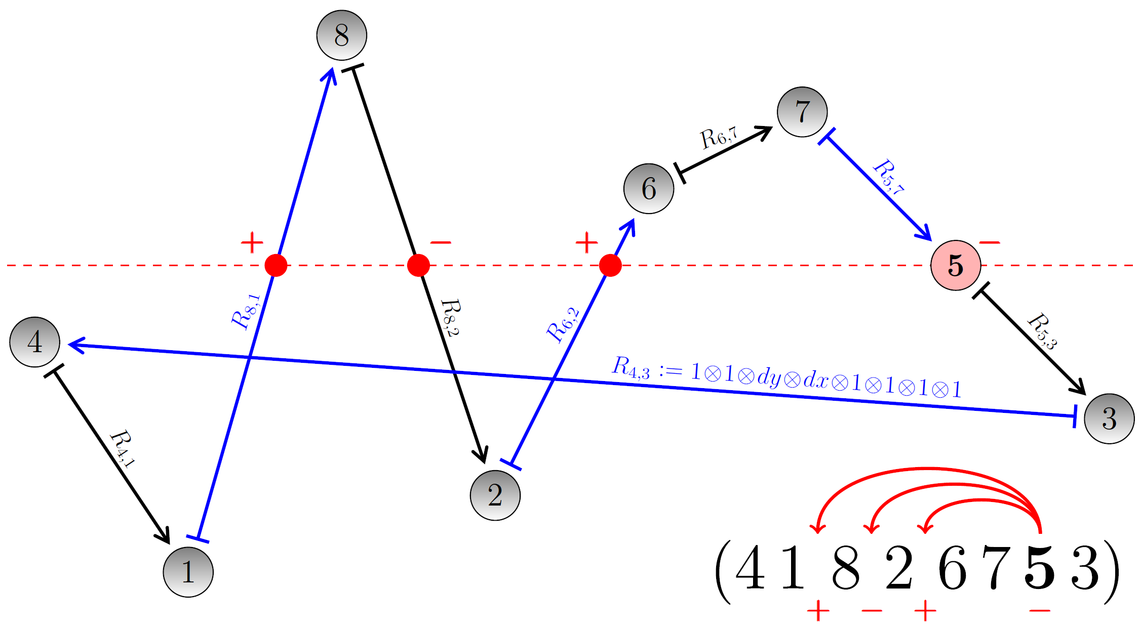
Figure 1: The cyclic permutation $\operatorname{\mathfrak{s}}=(4,1,8,2,6,7,5,3)$ with smallest transit $h=5$.

One half of the permutations that we obtain will have positive sign, one half negative sign. Removal and reinsertion of a smallest transit yields an equivalence relation $\sim$ on $\mathcal{D}_{2m}^{\prime}$, $\operatorname{\mathfrak{s}}\sim\operatorname{\mathfrak{r}}$ if and only if $\operatorname{\mathfrak{s}}^{\prime}=\operatorname{\mathfrak{r}}^{\prime}$. The corresponding equivalence classes form a partition of $\mathcal{D}_{2m}^{\prime}$, and each of them cancels off nicely. So, we only have to sum over $\mathcal{D}_{2m}\!\setminus\!\mathcal{D}_{2m}^{\prime}$, that is, over all permutations $\operatorname{\mathfrak{s}}\in\mathcal{S}_{2m}$ with

$$\text{either}\quad\operatorname{\mathfrak{s}}^{-1}(j)<j>\operatorname{\mathfrak{s}}(j)\quad\text{or}\quad\operatorname{\mathfrak{s}}^{-1}(j)>j<\operatorname{\mathfrak{s}}(j)$$ (39)

for all $j\in V:=\{1,2,\dotsc,2m\}$. We call this kind of permutations forth-back permutations. Their number is the so-called Euler zigzag number $A_{2m}$, i.e. $|\mathcal{D}_{2m}\!\setminus\!\mathcal{D}_{2m}^{\prime}|=A_{2m}$, as shown in Lemma 8 in the appendix. Since all forth-back permutations have sign $(-1)^{m}$, we get

$$w_{2m}\,=\,(2m)!\,A_{2m}.$$ (40)

From this and Equation (26) we finally arrive at Lévy’s classical result (3):

Theorem 7

The nonzero moments of the Lévy area $\mathcal{A}_{[a,b)}$ are

$$\mathbb{E}\!\left[\mathcal{A}_{[a,b)}\right]^{2m}\,=\,\,\left(\frac{b-a}{2}\right)^{\!2m}\!A_{2m}\,.$$

5 Appendix about Euler Numbers

In this section, we present a simple lemmas about Euler numbers. It is of sufficient general nature to be of potential interest elsewhere. Many similar results and basics can be found in [18] and [19].

A permutation $\mathfrak{s}$ in the symmetric group $\mathcal{S}_{n}$ is a zigzag permutation (misleadingly also called alternating permutation) if $\mathfrak{s}(1)>\mathfrak{s}(2)<\mathfrak{s}(3)>\mathfrak{s}(4)<\dotsb$. In other words, $\mathfrak{s}$ is zigzag if $\mathfrak{s}(1)>\mathfrak{s}(2)$ and

$$\text{either}\quad\mathfrak{s}(j-1)<\mathfrak{s}(j)>\mathfrak{s}(j+1)\quad\text{or}\quad\mathfrak{s}(j-1)>\mathfrak{s}(j)<\mathfrak{s}(j+1)$$ (41)

for all $j\in\{2,3\dotsc,n-1\}$. If we have the initial condition $\mathfrak{s}(1)<\mathfrak{s}(2)$, instead of $\mathfrak{s}(1)>\mathfrak{s}(2)$, we may call $\mathfrak{s}$ zagzig. The number of all zigzag permutations in $\mathcal{S}_{n}$ is called the Euler zigzag number $A_{n}$. These numbers occur in many places, for example, as the coefficients of $\frac{z^{2n}}{(2n)!}$ in the Maclaurin series of $\sec(z)+\tan(z)$. In this paper, we met them as the number of forth-back permutations, as we called them. These are the permutations $\mathfrak{s}\in\mathcal{S}_{n}$ with

$$\text{either}\quad\mathfrak{s}^{-1}(j)<j>\mathfrak{s}(j)\quad\text{or}\quad\mathfrak{s}^{-1}(j)>j<\mathfrak{s}(j)$$ (42)

for all $j\in\{1,2,\dotsc,n\}$. Since no forth-back permutation can contain a cycle of odd length, $n$ must be even for there to exist forth-back permutations, say $n=2m>0$. In that case, we actually have the following lemma:

Lemma 8

The number of forth-back permutations in $\mathcal{S}_{2m}$ is the Euler zigzag number $A_{2m}$.

Proof. A bijection between the forth-back permutations $\mathfrak{s}$ and the zigzag permutations in $\mathcal{S}_{2m}$ is obtained by applying the so-called transformation fundamentale [4]. To perform this transformation, we write $\mathfrak{s}$ in cycle notation

$$\mathfrak{s} = (\mathfrak{s}_{1},\mathfrak{s}_{2},\dotsc,\mathfrak{s}_{\ell_{2}-1})(\mathfrak{s}_{\ell_{2}},\mathfrak{s}_{\ell_{2}+1},\dotsc,\mathfrak{s}_{\ell_{3}-1})(\mathfrak{s}_{\ell_{3}},\mathfrak{s}_{\ell_{3}+1},\dotsc,\mathfrak{s}_{\ell_{4}-1})\dotsm$$ (43)

$$(\mathfrak{s}_{\ell_{m}},\mathfrak{s}_{\ell_{m}+1},\dotsc,\mathfrak{s}_{2m})\,.$$

This representation and the numbers  $\mathfrak{s}_{j}$ are uniquely determined if we require that the first entry of every cycle is bigger than all other entries in that cycle, and also that $\mathfrak{s}_{1}<\mathfrak{s}_{\ell_{2}}<\mathfrak{s}_{\ell_{3}}<\dotsb<\mathfrak{s}_{\ell_{m}}$. The new permutation $\mathfrak{\bar{s}}$ is then obtained by forgetting brackets and setting $\mathfrak{\bar{s}}(j):=\mathfrak{s}_{j}$. We just have to see that this actually yields a bijection $\mathfrak{s}\mapsto\mathfrak{\bar{s}}$ between forth-back and zigzag permutations. To do this we procede as follows.

Assume first that $\mathfrak{s}$ is forth-back. Then all cycles necessarily have even length and the permutation $\mathfrak{\bar{s}}$ is obviously zigzag, $\mathfrak{s}_{1}>\mathfrak{s}_{2}<\mathfrak{s}_{3}>\mathfrak{s}_{4}<\dotsb>\mathfrak{s}_{2m}$. Conversely, let us show that every zigzag permutation $\bar{\mathfrak{s}}$ has a unique pre-image $\mathfrak{s}$, and that that pre-image is forth-back. To construct a pre-image $\mathfrak{s}$ of $\bar{\mathfrak{s}}$, we only need to find suitable numbers $\ell_{j}$, which indicate where we have to insert brackets into the sequence $(\mathfrak{s}_{1},\mathfrak{s}_{2},\dotsc,\mathfrak{s}_{2m}):=(\mathfrak{s}(1),\mathfrak{s}(2),\dotsc,\mathfrak{s}(2m))$ to actually get a pre-image. However, if we have already found $\ell_{2},\ell_{3},\dotsc,\ell_{j}$, then $\ell_{j+1}$ is necessarily the first index $x$ with $\mathfrak{s}_{x}>\mathfrak{s}_{\ell_{j}}$. Using this, we can construct a pre-image $\mathfrak{s}$ of $\bar{\mathfrak{s}}$ in $\mathcal{S}_{2m}$, and it is uniquely determined. Moreover, if $\bar{\mathfrak{s}}$ is zigzag then this construction ensures that $\mathfrak{s}_{1}$ and the $\mathfrak{s}_{\ell_{j}}$ are peaks and their neighbors and $\mathfrak{s}_{2m}$ are valleys. Since also $\mathfrak{s}_{1}>\mathfrak{s}_{\ell_{2}-1}$, $\mathfrak{s}_{\ell_{2}}>\mathfrak{s}_{\ell_{3}-1}$, …, $\mathfrak{s}_{\ell_{m}}>\mathfrak{s}_{2m}$, insertion of brackets before the peaks $\ell_{j}$ yields forth-back cycles in $\mathfrak{s}$.

With the bijection established, it is now clear that there are as many forth-back permutations as there are zigzag permutations in $\mathcal{S}_{2m}$. This number is the Euler zigzag number $A_{2m}$.   

The number of forth-back permutations with just one cycle is given by the following lemma, which we present here as we think that it can be helpful in future research. If $\mathcal{C}_{n}$ denotes the subset of cyclic permutations in $\mathcal{S}_{n}$, we have the following:

Lemma 9

The number of forth-back permutations in $\mathcal{C}_{2m}$ is $A_{2m-1}$.

Proof. The cycle notation $\mathfrak{s}=(\mathfrak{s}_{1},\mathfrak{s}_{2},\dotsc,\mathfrak{s}_{2m})$ of cyclic permutations $\mathfrak{s}\in\mathcal{S}_{2m}$ is not uniquely determined, as one may rotate the entries cyclically. It becomes uniquely determined if we require that $\mathfrak{s}_{2m}=2m$. In this case, removal of the last entry yields a sequence $(\mathfrak{s}_{1},\mathfrak{s}_{2},\dotsc,\mathfrak{s}_{2m-1})$ that is zagzig (with $\mathfrak{s}_{1}<\mathfrak{s}_{2}$ as $\mathfrak{s}_{2m}$ was the biggest entry of $\mathfrak{s}$). If we define $\bar{\mathfrak{s}}\in\mathcal{S}_{2m-1}$ by setting $\bar{\mathfrak{s}}(j):=\mathfrak{s}_{j}$, for $j=1,2,\dotsc,2m-1$, we obtain a bijection $\mathfrak{s}\mapsto\bar{\mathfrak{s}}$ from the cyclic forth-back permutations in $\mathcal{S}_{2m}$ to the zagzig permutations in $\mathcal{S}_{2m-1}$. Indeed, every zagzig permutation $\bar{\mathfrak{s}}$ in $\mathcal{S}_{2m-1}$ has the cycle $\mathfrak{s}:=(\bar{\mathfrak{s}}(1),\bar{\mathfrak{s}}(2),\dotsc,\bar{\mathfrak{s}}(2m-1),2m)$ as unique pre-image. The existence of this bijection shows that the number of cyclic forth-back permutations in $\mathcal{S}_{2m}$ is equal to the number of zagzig permutations in $\mathcal{S}_{2m-1}$, which is $A_{2m-1}$, as for zigzag permutations.

References

[1] N. Bourbaki, Algebra I, Addison-Wesley, Reading MA (1974)
[2] Higher order Itô product formula and generators of
evolutions and flows, International Journal of Theoretical Physics 34, 1-6 (1995).
[3] S. Chen and R. L. Hudson, Some properties of quantum Lévy area
in Fock and non-Fock quantum stochastic calculus, Probability and Mathematical
Statistics 33, 425-434 (2013).
[4] D. Foata and M. Schützenberger, Théorie géométrique des polynómes eulériens, Springer Lecture Notes in Mathematics,
138 (1970).
[5] K. Helmes and A. Schwane, Lévy’s stochastic area formula in
higher
dimensions. Journal of functional analysis, 54.2, 177-192 (1983).
[6] M. Hoffman, The algebra of multiple harmonic series, Journal of Algebra
194, 477-495 (1997).
[7] R. L. Hudson, Sticky shuffle Hopf algebras and their stochastic
representations, pp165-181. in New trends in stochastic analysis and related
topics, A volume in honour of K D Elworthy, Ed H Zhao and A Truman, World
Scientific (2012).
[8] R. L. Hudson, Quantum Lévy area as a quantum martingale limit, pp
169-188, in Quantum probability and Related Topics XXIX, eds L Accardi and
F Fagnola, World Scientific (2013) .
[9] R. L. Hudson and J. M. Lindsay, A non-commutative martingale
representation theorem for non-Fock quantum Brownian motion, Journal of
Functional Analysis 61, 202–221 (1985).
[10] R. L. Hudson, U. Schauz and Y. Wu, Moments of quantum Lévy
areas using sticky shuffle Hopf algebras, ArXiv 1605.00730.
[11] D. Levin and M. Wildon, A combinatorial method of calculating the
moments of Lévy area, Trans. Amer. Math. Soc. 360, 6695-6709 (2008).
[12] P. Lévy, Le mouvement Brownien plan, Amer. Jour. Math. 62,
487-550 (1940).
[13] P. Lévy, Processus stochastiques et mouvement Brownien,
Gauthier-Villars, Paris (1948).
[14] P. Lévy, Calcul des probabilités-fonctions aléatoires
Laplaciennes, C. R. Acad. Sci. Paris Ser. A-B 229, 1057-1058 (1949).
[15] P. Lévy, Calcul des probabilités-sur l’aire comprise entre un arc
de la courbe du mouvement Brownien plan et sa corde, C. R. Acad. Sci. Paris Ser.
A-B 230, 432-434 (1950).
[16] P. Lévy, Wiener’s random function and other Laplacian functions, pp
171-187, in Proc. 2nd Berkeley Symposium Math Statistics and Probability 1950,
University of California Press (1951).
[17] K. R. Parthasarathy, An introduction to quantum stochastic
calculus, Birkhäuser (1992).
[18] T. K. Petersen, Eulerian Numbers, Birkhäuser (2015).
[19] R. P. Stanley, A survey of alternating permutations, Contemporary
Mathematics 531, 165-196 (2010).
[20] M. Yor, Remarques sur une formule de Paul Lévy,
Séminaire de Probabilités XIV, Lect. Notes in Maths. 784,
Springer-Verlag, Berlin (1980).