Efficient Timestamps for Capturing Causality

June 17, 2016

Abstract

Consider an asynchronous system consisting of processes that communicate via message-passing. The processes communicate over a potentially incomplete communication network consisting of reliable bidirectional communication channels. Thus, not every pair of processes is necessarily able to communicate with each other directly.

The goal of the algorithms discussed in this paper is to assign timestamps to the events at all the processes such that (a) distinct events are assigned distinct timestamps, and (b) the happened-before relationship between the events can be inferred from the timestamps. We consider three types of algorithms for assigning timestamps to events: (i) Online algorithms that must (greedily) assign a timestamp to each event when the event occurs. (ii) Offline algorithms that assign timestamps to event after a finite execution is complete. (iii) Inline algorithms that assign a timestamp to each event when it occurs, but may modify some elements of a timestamp again at a later time.

For specific classes of graphs, particularly star graphs and graphs with connectivity $\geq 1$, the paper presents bounds on the length of vector timestamps assigned by an online algorithm. The paper then presents an inline algorithm, which typically assigns substantially smaller timestamps than the optimal-length online vector timestamps. In particular, the inline algorithm assigns timestamp in the form of a tuple containing $2c+2$ integer elements, where $c$ is the size of the vertex cover for the underlying communication graph.

1 Introduction

Consider an asynchronous system consisting of $n$ processes that communicate via message-passing. The processes communicate over a potentially incomplete network of reliable bidirectional communication channels. The goal of the algorithms discussed in this paper is to assign timestamps to the events at all the processes such that (a) distinct events are assigned distinct timestamps, and (b) the happened-before [9] relationship between the events can be inferred from the timestamps.

We will consider three types of algorithms for assigning timestamps to events. To allow us to compare their behavior, let us introduce a query abstraction for timestamps. For event $e$, we use $e_{r}$ to denote the abstract real time (which is not available to the processes themselves) when event $e$ occurred. The timestamp of event $e$ may be queried at any real time $t$, $t\geq e_{r}$. Depending on the timestamp algorithm in use, the query may or may not return immediately. Denote by $Q^{t}(e)$ the timestamp that would be returned if a query were to be issued at real time $t$ for the timestamp of event $e$. Note that $Q^{t}(e)$ is defined even if no query is actually issued at time $t$. Also note that $Q^{t}(e)$ is only defined if $t\geq e_{r}$. The delay in computing $Q^{t}(e)$ depends on the algorithm for assigning timestamps, as seen below. Now let us introduce three types of timestamp algorithms:

• Online algorithms: An online algorithm must (greedily) assign a distinct timestamp to each event when the event occurs. Suppose that $\tau(e)$ is the timestamp assigned to event $e$ by an online algorithm. The assigned timestamps must be such that, for any two events $e$ and $f$, $e\rightarrow f$ iff $\tau(e)<\tau(f)$, where $<$ is a suitably defined partial order on the timestamps, and $\rightarrow$ is the happened-before relation [9]. The vector timestamp algorithm [4, 10] is an example of an online algorithm. For an online algorithm, for any event $e$, $Q^{t}(e)=\tau(e)$ for $t\geq e_{r}$; thus, a query issued at time $t\geq e_{r}$ can immediately return $Q^{t}(e)$.

• Offline algorithms: An offline algorithm takes an entire (finite) execution as its input, and assigns a distinct timestamp to each event in the execution. Similar to online algorithms, the timestamps $\tau(.)$ must be such that, for any two events $e$ and $f$, $e\rightarrow f$ iff $\tau(e)<\tau(f)$, where $<$ is a suitably defined partial order on the timestamps. There is significant past work on such offline computation of timestamps [1]. For an offline algorithm, query for the timestamp of any event will not return until the entire (finite) execution is complete, and the offline algorithm has subsequently computed the timestamps for the events.

• Inline algorithms: Timestamp assigned to an event by an inline algorithm may change as the execution proceeds. Thus, for an event $e$ it is possible that $Q^{t1}(e)\neq Q^{t2}(e)$ for $t2>t1\geq e_{r}$. However, timestamps for distinct events must be always distinct. That is, for distinct events $e$ and $f$, $Q^{t}(e)\neq Q^{v}(f)$ for any $t\geq max(e_{r},f_{r})$ We refer to timestamps assigned by inline algorithms as inline timestamps. A suitable partial order $<$ is defined on the inline timestamps. The inline timestamps must satisfy the following property for any two events $e$ and $f$ and for any $t\geq max(e_{r},f_{r})$,

  $Q^{t}(e)<Q^{t}(f)$ if and only if $e\rightarrow f$.

  Thus, the timestamps returned to queries at time $t$ must capture happened-before relation between events that have occurred by that time; however, $Q^{t}(e)$ may not suffice to infer happened-before relation with some other event $g$ where $g_{r}>t$. As an example, suppose that $e\rightarrow g$. Then, it is possible that $Q^{e_{r}}(e)\not<Q^{g_{r}}(g)$; however, as noted above, it must be true that $Q^{g_{r}}(e)<Q^{g_{r}}(g)$.

The inline algorithm presented in Section 4 has close similarities to mechanisms introduced previously for shared memory [8, 17] and message-passing [6, 7]. We will elaborate on the similarities (and differences) later in Section 5. Despite the past work, it appears that the ideas presented here have some novelty, as elaborated in Section 5.

2 System Model and Notation

We consider an asynchronous system. The $n$ processes in the system are named $p_{i}$, $0\leq i<n$. Processes communicate via reliable bidirectional message-passing channels. The communication graph for the system includes only undirected edges, and is denoted by $\mathcal{G}(\mathcal{P},\mathcal{E})$. $\mathcal{P}=\{p_{0},p_{1},\cdots,p_{n-1}\}$ denotes the set of vertices, where vertex $p_{i}$ represents process $p_{i}$. $\mathcal{E}$ is the set of undirected edges, where the undirected edge between $p_{i}$ and $p_{j}$, $p_{i}\neq p_{j}$, represents a bidirectional link.

The events are of three types: send events, receive events, and computation events. We consider only unicasts, thus, each send event results in a message sent to exactly one process. However, the proposed algorithm can be easily adapted when multiple messages may be sent at a single send event.

For an event $e$, proc(e) denotes the process at which event $e$ takes place. $\rightarrow$ denotes the happened-before relation between events [9]. For events $e$ and $f$, when $e\rightarrow f$, we say that “$f$ happened-after $e$”. If $e$ is a send event, then $recv(e)$ is the receive event at the recipient process for the message sent at event $e$. Recall that for event $e$, $e_{r}$ denotes the real time at which $e$ occurs. Different events at the same process occur at different real times. That is, if $e\neq f$ and $proc(e)=proc(f)$, then $e_{r}\neq f_{r}$.

For an event $e$, index(e) denotes the index of event $e$ at process proc(e). For convenience, define $index(\perp)=\infty$. In Figure 2(a), for event $g$, proc(g) = $p_{3}$ and index(g) = 2, because $g$ is the second event at $p_{3}$. For an event $e$ at a process $p_{i}$, and a process $p_{j}\neq p_{i}$, we define events $\mbox{\em outbound}(p_{j},e)$ and $\mbox{\em inbound}(p_{j},e)$ as follows:

• $\mbox{\em outbound}(p_{j},e)$ at time $t\geq e_{r}$ denotes the event at $p_{i}$ where $p_{i}$ sends the first message to $p_{j}$ at or after event $e$. If $p_{i}$ has not sent such a message by time $t$, then $\mbox{\em outbound}(p_{j},e)=\perp$ at time $t$. In particular, if $p_{i}$ sends a message to $p_{j}$ at event $e$, then $\mbox{\em outbound}(p_{j},e)=e$; otherwise, after event $e$, if process $p_{i}$ sends the first message to $p_{j}$ at some event $f$ such that $f_{r}\leq t$, then $\mbox{\em outbound}(p_{j},e)=f$ at time $t$.

• $\mbox{\em inbound}(p_{j},e)$ at any time $t\geq e_{r}$ is defined as follows: (i) If $\mbox{\em outbound}(p_{j},e)=\perp$ at time $t$, then $\mbox{\em inbound}(p_{j},e)=\perp$. (ii) Else $\mbox{\em inbound}(p_{j},e)=recv(\mbox{\em outbound}(p_{j},e))$. It is possible that, even when $\mbox{\em outbound}(p_{j},e)\neq\perp$ at time $t$, the receive event $recv(\mbox{\em outbound}(p_{j},e))$ may not yet be known – thus, although $\mbox{\em inbound}(p_{j},e)$ may be well-defined at time $t$, its value (i.e., $recv(\mbox{\em outbound}(p_{j},e))$) may not be known until later. As we will see later, this affects the design of the inline algorithm in Section 4.

Let ${\bf 0}$ denote a vector with all elements being 0; size of the vector is determined by the context. Similarly, let $\bm{\infty}$ denote a vector with all elements being $\infty$. $V[j]$ denotes element of vector $V$ at index $j$. Unless stated otherwise, for a vector of length $m$, we index its elements as 0 through $m-1$. For vectors $U$ and $V$ of equal size, $\max(U,V)$ is a vector obtained by taking their element-wise maximum. That is, the $j$-th element of vector $\max(U,V)$ equals $\max(U[j],V[j])$.

3 Vector Timestamps with Online Algorithms

The proposed inline algorithm in Section 4 assigns timestamps whose size depends on the vertex cover for the communication graph. A vertex cover of $\mathcal{G}(\mathcal{P},\mathcal{E})$ is a subset $\mathcal{C}$ of $\mathcal{P}$ such that each edge in $\mathcal{E}$ is incident on at least one vertex in $\mathcal{C}$. In particular, consider a star graph in which each process $p_{i}$, $i\neq 0$, has a link only with process $p_{0}$; there are no other links in a star graph. $p_{0}$ is the central process of the star graph, other processes being radial processes. The star graph has a vertex cover $\{p_{0}\}$ of size 1, and thus, the proposed inline algorithm assigns the smallest timestamps for star graphs. For comparison, we now present some bounds on timestamps assigned by online algorithms for some special classes of graphs, including star graphs. Let us define vector timestamps formally [1].

Vector timestamps:

Suppose that a given online algorithm assigns to each event $e$ a timestamp $\tau(e)$ consisting of a vector of a certain fixed size. These timestamps are said to be vector timestamps provided that $\tau(e)<\tau(f)$ iff and only if $e\rightarrow f$, where the partial order $<$ on timestamp vectors (such as $\tau(e)$ and $\tau(f)$) is defined as follows: For vectors $U$ and $V$, $U<V$ iff (a) $\forall j$ $U[j]\leq V[j]$, and (b) $\exists i$ such that $U[i]<V[i]$.

Vector timestamps are well-studied, and it has been shown that, in general, the vector length must be at least $n$ in the worst case even if the timestamps are assigned by an offline algorithm [1].

For online algorithms, and special classes of graphs, we show the following bounds on the length of the vector timestamps necessary to capture causality (i.e., $\tau(e)<\tau(f)$ iff $e\rightarrow f$). It appears that these bounds have not been obtained previously.

• Star graphs:

  • Real-valued vector elements: For $n\geq 3$, when the vector elements may take any finite real-value, $n-1$ is the tight bound for vector timestamp length for the star communication graph when using an online algorithm. Lemma 1 presented at the end of this section proves the lower bound of $n-1$, and Appendix B.2 presents an online algorithm, which constructively proves that $n-1$ is also an upper bound for $n\geq 3$.

    For $n=2$, vector length of 2 can be shown to be necessary and sufficient.

  • Integer-valued vector elements: When the vector elements are constrained to take integer values, $n$ is the tight bound for vector timestamp length for the star communication graph when using an online algorithm. Lemma 2 in Appendix B.1 proves the lower bound of $n$. Upper bound of $n$ is achieved by the standard vector clock algorithm [4, 10].

• Graphs with vertex connectivity = $\kappa$:

  • Vertex connectivity $\kappa\geq 2$: For any communication graph with vector connectivity $\kappa\geq 2$, Lemma 3 in Appendix B.3 proves that an online algorithm must use a vector timestamp of length $n$ in the worst case. Upper bound of $n$ is achieved by the standard vector clock algorithm [4, 10].

  • Vertex connectivity $\kappa=1$: For any given communication graph with vertex connectivity of $\kappa=1$, define $X$ to be the set of processes such that no process in set $X$ by itself forms a vertex cut of size 1. Then, as shown in Lemma 4 in Appendix B.3, $|X|$ is a lower bound on the vector size used by an online algorithm. Note that for the star graph, $|X|=n-1$.

While the above results for star graph show that it is not possible to assign small timestamps using online algorithm, we presently do not know if a similar claim is true for offline algorithms in star graphs. Appendix C presents a preliminary result for $n=4$ that suggests that further investigation is necessary to resolve the question.

Lemma 1

Suppose that an online algorithm for the star graph assigns distinct real-valued vector timestamps to distinct events such that, for any two events $e$ and $f$, $e\rightarrow f$ if and only if $\tau(e)<\tau(f)$. Then the vector length must be at least $n-1$.

Proof:

The proof is trivial for $n\leq 2$. Now assume that $n\geq 3$. The proof is by contradiction. Suppose that a give online algorithm assigns vector timestamps of length $s\leq n-2$.

Let $e_{q}^{j}$ denote the $q$-th event at process $p_{j}$. Consider an execution that includes a send event $e_{1}^{i}$ at radial process $p_{i}$, $1\leq i\leq n-1$, where the radial process $p_{i}$ sends a message to the central process $p_{0}$. These $n-1$ send events are concurrent with each other. At process $p_{0}$, there are $n-1$ receive events corresponding to the above send events at the other processes. The execution contains no other events.

$\tau(e_{q}^{j})$ denotes the vector timestamp of length $s$ assigned to event $e_{q}^{j}$ by the online algorithm. Create a set $S$ of processes as follows: for each $l$, $0\leq l<s$, add to $S$ any one radial process $p_{j}$ such that $\tau(e_{1}^{j})[l]=\max_{1\leq i<n}\,\tau(e_{1}^{i})[l]$. Note that $\tau(e_{1}^{i})[l]$ is the $l$-th element of vector $\tau(e_{1}^{i})$. Clearly, $|S|\leq s\leq n-2$. Consider a radial process $p_{k}\not\in S$ (note that $p_{k}\neq p_{0}$). Such a process $p_{k}$ must exist since $|S|\leq n-2$, and there are $n-1$ radial processes.

Suppose that the message sent by process $p_{k}$ at event $e_{1}^{k}$ reaches process $p_{0}$ after all the other messages, including messages from all the processes in $S$, reach process $p_{0}$. That is, $e_{n-1}^{0}$ is the receive event for the message sent by process $p_{k}$. By the time event $e_{n-1}^{0}$ occurs, (online) timestamps must have been assigned to all the other events in this execution. This scenario is possible because the message delays can be arbitrary, and an online algorithm assigns timestamps to the events when they occur.

Now consider event $e_{n-2}^{0}$. By event $e_{n-2}^{i}$, except for the message sent by process $p_{k}$, all the other messages, including messages sent by all the processes in $S$, are received by process $p_{0}$.

Define vector $E$ such that $E[l]=\max_{1\leq i<n}\,\tau(e_{1}^{i})[l]$, $0\leq l<s$. By definition of $S$, we also have that $E[l]=\max_{p_{i}\in S}\,\tau(e_{1}^{i})[l]$, $0\leq l<s$. The above assumption about the order of message delivery implies that $E\leq\tau(e_{n-2}^{0}).$ Also, since $p_{k}\not\in S$, we have that $\tau(e_{1}^{k})\leq E.$ The above two inequalities together imply that $\tau(e_{1}^{k})\leq\tau(e_{n-2}^{0})$.

Since $e_{1}^{k}\neq e_{n-2}^{0}$, their timestamps must be distinct too. Therefore, $\tau(e_{1}^{k})<\tau(e_{n-2}^{0})$, which, in turn, implies that $e_{1}^{k}\rightarrow e_{n-2}^{0}$. However, $e_{1}^{k}$ and $e_{n-2}^{0}$ are concurrent, leading to a contradiction. $\Box$

4 Inline Algorithm

The structure of the inline timestamps presented here has close similarities to comparable objects introduced in past work, in the context of message-passing [6, 7] and causal memory systems [8, 17]. We discuss the related work in Section 5, and also describe the extra flexibility offered by our approach.

The proposed inline algorithm makes use of a vertex cover for the given communication graph. Let $\mathcal{C}$ be the chosen vertex cover. It is assumed that each process knows the cover set $\mathcal{C}$. Define $c=|\mathcal{C}|$. Without loss of generality, suppose that the processes are named such that $\mathcal{C}=\{p_{0},p_{1},\cdots,p_{c-1}\}$.

The algorithm assigns a timestamp $\tau(e)$ to each event $e$. The timestamp for an event at each process $\mathcal{C}$ consists of just a vector of size $c$. On the other hand, the timestamp for an event at a process outside $\mathcal{C}$ includes other components as well. We refer to the vector component in a timestamp $\tau(e)$ as $\tau(e).vect$. The other components of the timestamp assigned to an event outside $\mathcal{C}$ are $id$, $index$ and $next$ (elaborated below).

The algorithm assigns an initial timestamp to each event $e$ when the event occurs. The vect field of a timestamp is not changed subsequently. Similarly, the index field, present only in timestamps of events outside $\mathcal{C}$, is also not changed subsequently. The $next$ field of the timestamp, assigned only to an event outside $\mathcal{C}$, however, may be updated as the execution progresses beyond the event (as elaborated below). Since the timestamps for events in $\mathcal{C}$ only include the $vect$ field, it follows that the once a timestamp is assigned to an event in $\mathcal{C}$, it is never modified.

Intuition behind inline timestamps:

The inline algorithm exploits the fact that at least one endpoint of each communication channel must be at a process in $\mathcal{C}$. In particular, for an event $e$ that occurs at a process outside $\mathcal{C}$, the algorithm identifies the most recent event in $\mathcal{C}$, say $f$, such that $f\rightarrow e$. Similarly, for an event $e$ that occurs outside $\mathcal{C}$, the algorithm identifies the earliest event at each $p_{j}\in\mathcal{C}$, say event $f_{j}$, that happened-after $e$ and is influenced directly by the process where $e$ occurs. Here “influence directly” means that the process $proc(e)$ sends a message to $p_{j}$. Indices of these events are used to form the inline timestamp of event $e$. Since $proc(e)$ may “directly influence” different processes at different times, the corresponding components of the timestamp are updated accordingly when necessary.

For events at processes in $\mathcal{C}$, the inline algorithm uses the standard vector clock algorithm [4, 10], with the vector elements restricted to processes in $\mathcal{C}$. In particular, for an event $e$ at $p_{i}\in\mathcal{C}$, $\tau(e).vect$ is a vector of length $c$, and with the following properties:

• If $e$ is the $k$-th event at $p_{i}$, then $\tau(e).vect[i]=k$.

• For $p_{j}\in\mathcal{C}$ where $p_{j}\neq p_{i}$, $\tau(e).vect[j]$ is the number of events at $p_{j}$ that happened-before $e$.

4.1 Inline Algorithm Pseudo-Code

Each process $p_{i}$ maintains a local vector clock $clock_{i}$ of size $c$. Initially, $clock_{i}:={\bf 0}$. Consider a new event $e$ at process $p_{i}$. We now describe how the various fields of the timestamp are computed:

• If $p_{i}\not\in\mathcal{C}$ then $\tau(e).id:=p_{i}$ and $\tau(e).index:=index(e)$.

• $vect$ field:

  • If $p_{i}\in\mathcal{C}$, then $clock_{i}[i]:=clock_{i}[i]+1$.

  • If $e$ is a send event, then piggyback the following on the message sent at event $e$: (i) vector $clock_{i}$, and (ii) if $p_{i}\not\in\mathcal{C}$ then $\tau(e).index$.

  • If $e$ is a receive event, then let $v$ be the vector piggybacked with the received message, and update $clock_{i}:=\max(clock_{i},v).$

  • $\tau(e).vect:=clock_{i}$.

• $next$ field: If $p_{i}\in\mathcal{C}$, computation of $next$ is not performed.

  The steps performed when $p_{i}\not\in\mathcal{C}$ depend on the type of the event, as follows:

  1. $\tau(e).next:=\bm{\infty}$.

  2. If $e$ is a send event for message memor $m$ destined for some process $p_{j}\neq p_{i}$ then define an event set $N_{e}$ as follows:

     $$N_{e}~{}=~{}\{e\}\cup\{f~{}|~{}\mbox{$proc(f)=p_{i}$ and $f\rightarrow e$ and~{}}\tau(f).next[j]=\infty\}$$

  3. When $index(\mbox{\em inbound}(p_{j},e))$ becomes known to $p_{i}$, for each $g\in N_{e}$,

     $$\tau(g).next[j]:=index(\mbox{\em inbound}(p_{j},e))$$

     The discussion of how $p_{i}$ learns $index(\mbox{\em inbound}(p_{j},e))$ is included with the discussion of the query procedure in Section 4.2.

Observe that the algorithm essentially assigns vector timestamps to events in $\mathcal{C}$, with vector elements restricted to the processes in $\mathcal{C}$. The $next$ field for events outside $\mathcal{C}$ may change over time, as per steps 2 and 3 above.

4.2 Response to a Query for Timestamps

Consider any event $e$ that occurs at time $e_{r}$ at some process $p_{i}$. If by some time $v\geq e_{r}$, the event $\mbox{\em outbound}(p_{j},e)$ has occurred already, but $\tau(e).next[j]=\infty$, then the $next[j]$ field of timestamp $Q^{v}(e)$ of $e$ cannot yet be determined (refer to Step 3 of the algorithm above). Hence, the query for $Q^{v}(e)$ is delayed until this information becomes available to $p_{i}$. To allow $p_{i}$ to learn the index of the receive event for the message it sent to $p_{j}$ at event $\mbox{\em outbound}(p_{j},e)$, process $p_{j}$ can send a control message to $p_{i}$ carrying the index of its receive event, as well as the index of the corresponding send event at $p_{i}$ (the index of the send event is piggybacked on the application message, as specified in the pseudo-code above). Dashed arrows in Figure 2 illustrate such control messages. In particular, the last control message in Figure 2(b) carries index 5 of the receive event at $p_{1}$ and index 4 of the corresponding send event at $p_{3}$. Section 4.3 elaborates on the example in Figure 2

The overhead of the above control messages can potentially be mitigated by judiciously piggybacking control information on application messages. Alternatively, the control information can be “pulled” only when needed. In particular, when a query for timestamp of some event $e$ is performed at $p_{i}$ at time $v$, $p_{i}$ can send a control message to the processes in $\mathcal{C}$ to learn any event index information that may be necessary to return $Q^{v}(e)$.

To summarize, the response to a query for timestamps of event $e$ at process $p_{i}\not\in\mathcal{C}$ at time $v\geq e_{r}$ is handled as follows:

• While ($\exists p_{j}\in\mathcal{C}$ such that $\mbox{\em outbound}(p_{j},e)\neq\perp$, and $\tau(e).next[j]=\infty$) wait.

• Return $\tau(e)$ as $Q^{v}(e)$.

4.3 Example of Inline Timestamps and Query Procedure

Figure 1: An example communication graph

Consider the communication network in Figure 1. For this network, let us choose $\mathcal{C}=\{p_{0},p_{1}\}$. Thus, the timestamps for events at processes in $\mathcal{C}$ (i.e., $p_{0}$ and $p_{1}$) consist of a vector of length 2. Figure 2(a) shows all the events that have taken place in a certain execution by time $t$. In this execution, the initial timestamp $Q^{e_{r}}(e)$ for event $e$ at $p_{0}$ is (3,1) because it is the third event at process $p_{0}$, and only one event at $p_{1}$ happened-before event $e$ (this dependence arises due to messages exchanged by $p_{0}$ and $p_{1}$ with process $p_{3}\not\in\mathcal{C}$). The timestamp for an event in $\mathcal{C}$ does not change after the initial assignment. Thus, $Q^{e_{r}}(e)=Q^{t}(e)$ for any $t>e_{r}$. The solid arrows in the figure depict application messages, whereas the dashed arrow depicts a control message, to be explained later.

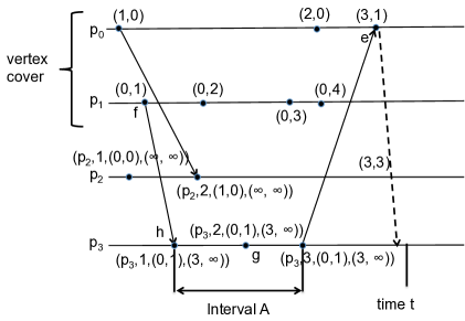
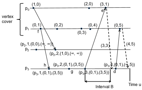
(a)                                                              (b)

Figure 2: (a) An execution showing all the events that have taken place by time $t$. For each event $x$ in the figure, timestamp $Q^{t}(x)$ returned for a query issued at $t$ is also shown. A solid arrow depicts an application messages, whereas dashed arrow depicts a control message. (b) Extended execution showing events that have taken place by time $u$, and timestamp $Q^{u}(x)$ for each event $x$.

In Figure 2(a), the timestamp $Q^{h_{r}}(h)$ of event $h$ when it occurs at $p_{3}$ at time $h_{r}$ is $(p_{3},1,(0,1),(\infty,\infty))$ – this timestamp is not depicted in the figure. However, at time $t$, as depicted in Figure 2(a), $Q^{t}(h)=(p_{3},1,(0,1),(3,\infty))$. The $index$ in the timestamp is 1 because $h$ is the first event at $p_{3}$. $vect=(0,1)$ in the timestamp because no event at $p_{0}$ and 1 event at $p_{1}$ happened-before event $h$. Observe that $vect$ field of $Q^{h_{r}}(h)$ and $Q^{t}(h)$ is identical. In fact, except the $next$ field, the other fields of the timestamps do not change after their initial assignment. Both the elements of $next$ in $Q^{h_{r}}(h)=(p_{3},1,(0,1),(\infty,\infty))$ are $\infty$, because $h$ is not a send event. Subsequently, if and when $p_{3}$ sends messages to processes in $\mathcal{C}$, corresponding elements of $next$ are updated. For instance, the $next[0]$ element of $Q^{t}(h)$ is $3$ because 3 is the index of the event $e$ at $p_{0}$ at which $p_{0}$ receives a message from $p_{3}$ that was sent at time $\geq h_{r}$ and $\leq t$. $next[1]$ in timestamp $Q^{t}(h)$ is $\infty$ because process $p_{3}$ does not send a message to process $p_{1}$ at any time between $h_{r}$ and $t$. Observe that the timestamp $Q^{t}(g)$ for event $g$ at $p_{3}$ differs from $Q^{t}(h)$ only in its $index$: the $vect$ and $next$ are identical for events $h$ and $g$. The dashed arrow in Figure 2(a) depicts a control message that allows process $p_{3}$ to learn the index of the event at $p_{0}$ where $p_{0}$ received a message from $p_{3}$. Process $p_{3}$ can determine, on receipt of the control message in Figure 2(a), that $Q^{t}(h).next[0]=3$.

For any $j$, once $next[j]$ is assigned a finite value, the field $next[j]$ is not modified again. For instance, in the above example, because $Q^{t}(h).next[0]=3$, it follows that $Q^{u}(h).next[0]=3$ for any $u>t$ as well. However, since $Q^{t}(h).next[1]$ is $\infty$, if at a later time, process $p_{3}$ were to send a message to $p_{1}$, $next[1]$ is updated appropriately. For instance, Figure 2(b) shows an extended version of the execution in Figure 2(a) that shows all the events that occur by some time $u>t$. Also, Figure 2(b) shows the timestamp $Q^{u}(x)$ corresponding to query at time $u$ for each event $x$ shown in the figure. Now observe that $next[1]$ for event $h$ and $g$ are both changed to 5, because the message sent by process $p_{3}$ to $p_{1}$ is received at the $5^{th}$ event at $p_{1}$. For event $d$ at $p_{3}$, while $next[1]$ equals 5 (similar to $next[1]$ for event $g$), $next[0]$ for event $d$ is presently $\infty$, since process $p_{3}$ is yet to send a message to $p_{0}$ (i.e., at or after event $d$).

Delay in responding to some queries:

In Figure 2(a), at any time $v$ during interval A, $Q^{v}(h)$ will be returned as $(p_{3},1,(0,1)(\infty,\infty))$ because process $p_{3}$ is yet to send any message after event $h$. In Figure 2(a), the dotted arrow is a control message that carries the index of event $e$ – on receipt of this message, $p_{3}$ learns $\mbox{\em inbound}(p_{0},h)$. In Figure 2(b), query issued anytime during interval B will have to wait until $p_{3}$ learns $\mbox{\em inbound}(p_{0},h)$. On the other hand, query at time $u$ in Figure 2(b) will return $Q^{u}(h)=(p_{3},1,(0,1),(3,5))$.

4.4 Inferring Happened-Before ($\rightarrow$) from the Inline Timestamps

Recall that timestamps for events at processes in $\mathcal{C}$ do not include an $id$ field, whereas timestamps for events at processes in $\mathcal{C}$ do include an $id$ field. In the following, we use the convention that, if $\tau_{1}$ is the timestamp for an event at a process in $\mathcal{C}$, then $\tau_{1}.id=\perp$. On the other hand, for timestamps of events at processes outside $\mathcal{C}$, $id\neq\perp$.

For the inline timestamps defined above, we define the $<$ relation as follows. Consider two inline timestamps $\tau_{1}$ and $\tau_{2}$. $\tau_{1}<\tau_{2}$ if and only if one of the following is true:

• (i)  $\tau_{1}.id=\tau_{2}.id\neq\perp$ and $\tau_{1}.index<\tau_{2}.index$, or

  (ii) $\tau_{1}.id=\tau_{2}.id=\perp$ and $\tau_{1}.vect<\tau_{2}.vect$, or

  (iii) $\tau_{1}.id=\perp$, $\tau_{2}.id\neq\perp$, and $\tau_{1}.vect\leq\tau_{2}.vect$, or

  (iv) $\tau_{1}.id\neq\perp$, $\tau_{1}.id\neq\tau_{2}.id$, and $\exists i,~{}0\leq i<c$, such that $(\tau_{1}.next[i]\leq\tau_{2}.vect[i])$.

The four cases above cover all possibilities. In particular, in case (i), the two events are at the same process outside $\mathcal{C}$. In case (ii), the two event are at processes (not necessarily identical) in $\mathcal{C}$. In case (iii), $\tau_{1}$ is timestamp of an event at a process in $\mathcal{C}$, whereas $\tau_{2}$ corresponds to an event outside $\mathcal{C}$. Finally, in case (iv), timestamp $\tau_{1}$ corresponds to an event at a process outside $\mathcal{C}$, whereas the event corresponding to $\tau_{2}$ may be at any other process (in or outside $\mathcal{C}$).

With the above definition $<$, the theorem below states that the inline algorithm satisfies the requirement that the timestamps be useful in inferring causality.

Theorem 1

For any two events $e$ and $f$, and for $t\geq max(e_{r},f_{r})$, $Q^{t}(e)$ and $Q^{t}(f)$ are the timestamps returned by the query procedure when using the proposed inline algorithm. The following condition holds:
                      $e\rightarrow f$   if and only if    $Q^{t}(e)<Q^{t}(f)$,
where partial order $<$ for inline timestamps is as defined above.

Appendix A presents the proof of this theorem. Appendix E discusses some implementation issues related to the inline algorithm.

5 Related Work

The concept of vector clock or vector timestamp was introduced by Mattern [10] and Fidge [4]. Charron-Bost [1] showed that there exist communication patterns that require vector timestamp length equal to the number of processes. Schwarz and Mattern [12] provided a relationship between the size of the vector timestamps and the dimension of the partial order specified by happened-before. Garg et al. [5] also demonstrated analogous bounds on the size of vector timestamps using the notion of event chains. Singhal and Kshemkalyani [14] proposed a strategy for reducing the communication overhead of maintaining vector timestamps. Shen et al. [13] encode of a vector clock of length $n$ using a single integer that has powers of $n$ distinct prime numbers as factors. Torres-Rojas and Ahmad propose constant size logical clocks that trade-off clock size with the accuracy with which happened-before relation is captured [15]. Meldal et al. [11] propose a scheme that helps determine causality between two messages sent to the same process. They observe that, because their timestamps do not need to capture the happened-before relation between all events, their timestamps can be smaller. Some of the algorithms presented by Meldal et al. [11] exploit information about the communication graph, particularly information about the paths over which messages may be propagated.

Closely related work:

Closest to our work is a timestamp algorithm for synchronous messages by Garg et al. [6, 7], timestamps used in causal memory implementations, particularly, Lazy Replication [8] and SwiftCloud [17], and a hierarchical cluster timestamping scheme [16]. We will discuss these prior schemes next.

Synchronous messages:

For synchronous messages, the sender process, after sending a message, must wait until it receives an acknowledgement from the receiver process. This constraint is exploited in [6, 7] to design small timestamps. In particular, if the communication network formed by the processes is decomposed into, say, $d$ components that are either triangles or stars, then the timestamps contain $d+4$ integer elements. Although our timestamps have similarities to the structure used in [6, 7], our algorithm does not constrain the messages to be synchronous. As a trade-off, our timestamps are somewhat larger than [6, 7]. In [6, 7], a sender process cannot take any additional steps until it receives an acknowledgement for a sent message. We do not impose this constraint. In particular, the delay in receiving the control messages in our case only delays response to timestamp queries, but not necessarily the computation at the processes.

Causal memory [8, 17]:

While there are close similarities between our work and timestamps maintained by causal memory schemes [8, 17], one critical difference is that our work focuses message passing whereas [8, 17] focuses on shared memory.

In Lazy Replication [8], each client sends its updates and queries to one of the servers. A server that receives an update from one of the clients then propagates the update to the other servers. Each server maintains a vector clock, similar to the timestamps at processes in our cover $\mathcal{C}$: the $i$-th entry of the vector at the $j$-server essentially counts the number of updates propagated to the $j$-th server by the $i$-th server. In essence, the servers are fully connected, whereas our cover $\mathcal{C}$ need not be. Each client also maintains a vector similar to $vect$ in timestamps for processes $\not\in\mathcal{C}$ in our case. Additionally, when a client sends its update to the $j$-th server, the $j$-th element of the client’s vector is updated to the index of the client’s update at the $j$-th server. The client may potentially send the same update to multiple servers, say, $j$-th and $k$-th servers; in this case, the $j$-th and $k$-th elements of the client’s vector will be updated to the indices of the client’s updates at the respective servers. The way the timestamps are compared in Lazy Replication differs slightly from the partial order defined on inline timestamps, because our goal is to capture causality exactly, whereas in Lazy Replication an approximation suffices – this is elaborated in Appendix D.

The mechanism used in SwiftCloud [17] is motivated by Lazy Replication [8], and has close similarities to the vectors in [8]. In SwiftCloud, if a client sends its update to multiple servers, then the indices returned by the servers are merged into the dependency vector maintained by the client (optionally, some of the returned indices may not be merged). Importantly, a server can only respond to future requests from the client provided that the server’s vector covers the client’s dependency vector. This has similarities to the manner in which we compare inline timestamps.

The size of the timestamps in above causal memory schemes is a function of the number of servers (that are completely connected to each other). On the other hand, we allow arbitrary communication networks, with the size of the timestamps depending on vertex cover size for the communication network. This enable alternative implementations.

For instance, consider a client-server architecture, wherein a large number of clients may interact with a large number of servers. Due to the dense communication (or interconnection) pattern in this case, the cover size will be large, resulting in large timestamps. An alternative is illustrated in Figure 3, where the solid edges represent an abstract communication network. A client or a server may communicate with multiple sequencers. By design, the sequencers form a cover of this network. When the number of servers is much larger than the number of sequencers, this approach can result in a much smaller vertex cover. In Figure 3, all communication must go through the sequencers, and the inline timestamp size is proportional to number of sequencers. However, routing all server communication via sequencers can be expensive, since the sequencers will have to handle a large volume of data. A simple optimization can mitigate this shortcoming. For example, as shown by a dashed arrow in Figure 3, server $R_{1}$ may send message contents (data) directly to server $R_{2}$, but server $R_{2}$ will need to wait to receive metadata, in the form of timestamp information, via sequencer $S_{1}$ (as shown by a dotted arrow in the figure). Thus, while the sequencers must still handle small messages to help determine inline timestamps, bulk of the traffic can still travel between the servers directly (or similarly between servers and clients). A similar optimization was suggested previously for totally-ordered multicast using a sequencer [2]. This optimization, in conjunction with our scheme, provides a trade-off between timestamp size and the delay incurred in routing metadata through sequencers.

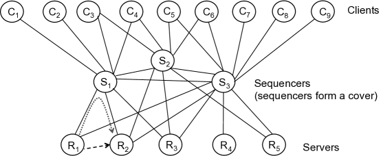
Figure 3: Alternate architecture suitable for inline timestamping

Cluster timestamps:

Ward and Taylor [16] describe an improvement over the strategy previously proposed by Summers, which divides the processes into clusters. They maintain short timestamps (proportional to cluster size) for events that occur inside the cluster, and longer timestamps (vectors with length equal to total number of processes) for “cluster-receive” events. In [16], the ”cluster-receive” events are assigned long timestamps; such long timestamps are not generally necessary in our case.

5.1 Causal Memory Systems with Smaller Timestamps

As discussed previously, causal memory systems use timestamp vectors analogous to the inline timestamps discussed in this paper. The causal memory systems maintain multiple replicas of the shared data, and require vectors whose size is equal to the number of replicas [17, 8]. When the number of replicas is large, the vector size becomes large. To mitigate this shortcoming, we can envision a modified architecture for causal memory, based on the idea illustrated in Figure 3 for a generic client-server systems. Each server can be viewed as a replica of the shared data. A suitable number of sequencers can be introduced to limit the size of the timestamps. Performance may be improved by using the optimization described above. The prior causal memory algorithms (such as [17]) can be easily adapted for the architecture in Figure 3, while incorporating timestamp objects based on inline timestamps (with size dependent on vertex cover size, instead of the total number of servers).

6 Summary

We exploit the knowledge of the communication graph to reduce timestamp size, while correctly capturing the happened-before relation. We present an algorithm for assigning inline timestamps, and show that the timestamps are often much smaller than vector timestamps assigned by online algorithms. Bounds on length of vector timestamps used by online algorithms are also presented.

Acknowledgements

The authors thank Vijay Garg, Ajay Kshemkalyani and Jennifer Welch for their feedback. We thank Marek Zawirski for answering questions about SwiftCloud [17].

Appendix

Appendix A Proof of Theorem 1: Correctness of Inline Algorithm

In this section, we prove Theorem 1, which claims that the timestamps provided by our inline algorithm can be used to capture causality. Recall that partial order on inline timestamps is defined in Section 4. For ease of reference, we define the partial order here again.

Consider two inline timestamps $\tau_{1}$ and $\tau_{2}$. $\tau_{1}<\tau_{2}$ if and only if one of the following is true:

• (i)  $\tau_{1}.id=\tau_{2}.id\neq\perp$ and $\tau_{1}.index<\tau_{2}.index$, or

  (ii) $\tau_{1}.id=\tau_{2}.id=\perp$ and $\tau_{1}.vect<\tau_{2}.vect$, or

  (iii) $\tau_{1}.id=\perp$, $\tau_{2}.id\neq\perp$, and $\tau_{1}.vect\leq\tau_{2}.vect$, or

  (iv) $\tau_{1}.id\neq\perp$, $\tau_{1}.id\neq\tau_{2}.id$, and $\exists i,~{}0\leq i<c$, such that $(\tau_{1}.next[i]\leq\tau_{2}.vect[i])$.

Proof of Theorem 1:

Proof:

Consider events $e$ and $f$. Let $t\geq\max(e_{r},f_{r})$. Let $\tau_{1}=Q^{t}(e)$ and $\tau_{2}=Q^{t}(f)$.

We consider four possibilities that take into account whether $e$ and $f$ occurred at processes in $\mathcal{C}$ or outside $\mathcal{C}$.

Case 1: Both $e$ and $f$ occur at processes in $\mathcal{C}$:  In this case, $\tau_{1}.id=\tau_{2}.id=\bot$. Hence, condition (ii) above applies. Since the processes in $\mathcal{C}$ implement the standard vector clock protocol, $e\rightarrow f$ if and only if $\tau_{1}.vect<\tau_{2}.vect$

Case 2: $e$ occurs at a process in $\mathcal{C}$ and $f$ occurs at a process outside $\mathcal{C}$:  In this case, condition (iii) applies. Also, $\tau_{1}.vect[i]$ (respectively, $\tau_{2}.vect[i]$) denotes the number of events on $p_{i}\in\mathcal{C}$ that happened-before $e$ (respectively, $f$). Thus, $e\rightarrow f$ if and only if $f$ is aware of all events that $e$ is aware of. Note that if $e$ happened before $f$ then $f$ is aware of at least one extra event than $e$. However, this extra event may not be on a process in $\mathcal{C}$. Thus, we have $e\rightarrow f$ iff $\tau_{1}.vect\leq\tau_{2}.vect$.

Case 3: $e$ occurs at a process outside $\mathcal{C}$ and $f$ occurs at a process in $\mathcal{C}$:  In this case, $\tau_{1}.next[i]$ denotes the earliest time (if it exists) such that there exists an event $g_{i}$ on process $p_{i}\in\mathcal{C}$ such that $g_{i}$ was created due to a message sent by the process where $e$ occurred and received by $p_{i}$. Since $e$ and $f$ are on different processes, $e\rightarrow f$ iff there exists $g_{i}$ on $p_{i}\in\mathcal{C}$ such that $f=g_{i}$ or $g_{i}\rightarrow f$. In the former case, by construction $\tau_{1}.next[i]=\tau_{2}.vect[i]$. In the latter case, $f$ is aware of at least one extra event on $\mathcal{C}$ that $g_{i}$ was aware of. Hence, if $e\rightarrow f$ then $\tau_{1}.next[i]\leq\tau_{2}.vect[i]$.

Also, if $\tau_{1}.next[i]\leq\tau_{2}.vect[i]$ then consider the event $g_{i}$ that is responsible for assignment of $\tau_{1}.next[i]$. Using the same argument above, $g_{i}=f$ or $g_{i}\rightarrow f$. Thus, if $\tau_{1}.next[i]\leq\tau_{2}.vect[i]$ then $e\rightarrow f$.

Case 4: Both $e$ and $f$ occur at processes outside $\mathcal{C}$:  Here, we consider two cases: If $e$ and $f$ are on the same process then condition (i) applies, and, $e$ happened before $f$ iff $e$ occurred (by real time) before $f$. In other words, $e\rightarrow f$ iff $\tau_{1}.index<\tau_{2}.index$. The second subcase where $e$ and $f$ occur at different processes outside $\mathcal{C}$ is similar to Case 3 except that $f$ and $g_{i}$ cannot be identical in Case 4.

$\Box$

Appendix B Bounds for Vector Timestamp Length with Online Algorithms

This appendix presents several bounds for the length of vector timestamps assigned by online algorithms. Recall that, for vector timestamps, the $<$ partial order is defined in Section 3.

In the discussion below, let $e_{q}^{i}$ denote the $q$-th event at process $p_{i}$.

B.1 Lower Bound for the Star Graph

Real-Valued Vector Timestamps:

Lemma 1 in Section 3 shows that $n-1$ is a lower bound on the vector timestamp length in star graphs when the elements of the vector may be real-valued. The lemma below derives a lower bound when the vector elements must be integer-valued.

Now we consider the case when the vector elements are constrained to be integer-valued.

Integer-Valued Vector Timestamps:

Lemma 2

Suppose that an online algorithm for the star graph assigns vector timestamps with integer-valued vector elements, such that, for any two events $e,f$, $e\rightarrow f$ iff $\tau(e)<\tau(f)$. Then the vector length must be at least $n$.

Proof:

Without loss of generality, let us assume that all vector elements of a vector timestamp must be non-negative integers. The proof of the lower bound is trivial for $n=1$. Now assume that $n\geq 2$. The proof is by contradiction. Suppose that the vector length is $s\leq n-1$.

Consider an execution that includes a send event $e_{1}^{i}$ at process $p_{i}$, $1\leq i\leq n-1$, where the radial process $p_{i}$ sends a message to the central process $p_{0}$. Let $M$ be the largest value of any of the $s$ elements of the timestamps of any of these $n-1$ send events. Suppose that process $p_{0}$ initially performs $P$ computation events. Assume that there are no other events; thus, process $p_{0}$ does not send any messages. Thus, the timestamps of the send events at the radial processes cannot depend on $P$, the number of computation events at $p_{0}$. Thus, we can assume that $P=(M+2)n$. Since these $(M+2)n$ computation events occur at $p_{0}$ before it receives any messages, the timestamps for these events are computed before $p_{0}$ learns timestamps of any send events at the other processes. Since the timestamp elements are constrained to be non-negative integers, one of the elements of the timestamp of the last of these computation events at $p_{0}$, namely $e_{Pn}^{0}$ must be $>M$. Recall that $P=(M+2)n$.

Consider set $W$ that contains event $e_{Pn}^{0}$ and $e_{1}^{i},~{}0<i<n$. Thus, $W$ contains $n$ events, with one event at each of the $n$ processes. Create a set $S$ of processes as follows: for each $l$, $0\leq l<s$, add to $S$ any one process $p_{j}$ such that the $l$-th element of the timestamp of its event in $W$ is the largest among the $l$-th elements of the timestamps of all the events in $W$. Clearly, $p_{0}\in S$ and $|S|\leq s\leq n-1$. Consider a radial process $p_{k}\not\in S$ (note that $p_{k}\neq p_{0}$). Such a process $p_{k}$ must exist since $|S|\leq n-1$, $p_{0}\in S$, and there are $n-1$ radial processes.

Suppose that the message sent by process $p_{k}$ at event $e_{1}^{k}$ reaches process $p_{0}$ after all the other messages, including messages from the radial processes in $S$, reach process $p_{0}$. Let $e=e_{Pn+n-2}^{0}$. By event $e$ at $p_{0}$, except for the message sent by process $p_{k}$, all the other messages, including messages sent by all the radial processes in $S$, are received by process $p_{0}$.

Rest of the proof of this lemma is similar to the proof of Lemma 1. In particular, define vector $E$ such that $E[l]=\max_{1\leq i<n}\,\tau(e_{1}^{i})[l]$, $0\leq l<s$. By definition of $W$, we also have that $E[l]=\max_{p_{i}\in W}\,\tau(e_{1}^{i})[l]$, $0\leq l<s$. The above assumption about the order of message delivery implies that

$$E\leq\tau(e_{Pn+n-2}^{0}).$$

Also, since $p_{k}\not\in W$, we have that $\tau(e_{1}^{k})\leq E$. This implies that $\tau(e_{1}^{k})\leq\tau(e_{Pn+n-2}^{0})$.

Since $e_{1}^{k}\neq e_{Pn+n-2}^{0}$, their timestamps must be distinct too. This implies that $\tau(e_{1}^{k})<\tau(e_{Pn+n-2}^{0})$, which, in turn, implies that $e_{1}^{k}\rightarrow e_{Pn+n-2}^{0}$. However, $e_{1}^{k}$ and $e_{Pn+n-2}^{0}$ are concurrent events, leading to a contradiction. $\Box$

B.2 Upper Bound for the Star Graph: Real-Valued Elements

For a star graph with $n=1,2$, it is easy to show that the vector length must be at least $n$, and also that vector length $n$ suffices using the standard vector clock algorithm. Thus, the bound of Lemma 1 is not tight for $n=1,2$.

In the rest of this section, we focus on $n\geq 3$.

Lemma 1 shows that $n-1$ is a lower bound on the vector length used by an online algorithm for star graphs. Now we constructively show that this bound is tight for $n\geq 3$ by presenting an online algorithm for computing vector timestamps of length $n-1$. The vector elements of timestamps assigned by the algorithm below are real-valued. (If the elements are constrained to be integers, then, as shown in Lemma 2, vector length of $n$ will be required.)

We first define a function $update$ that takes process identifier $p_{i}$ and a vector $w$ of length $n-1$ as its arguments, and returns an updated vector. The $n-1$ elements of the vector timestamps have indices 1 through $n-1$. Update performed by the central process $p_{0}$ is different than the update performed by the radial processes.

Function $update(p_{k},w)$

{

if ($p_{k}\neq p_{0}$)

$w[k]:=\lfloor w[k]+1\rfloor$     // smallest integer larger than the original value of $w[k]$

else

for $1\leq j\leq n-1,~{}~{}w[j]:=\mbox{any value in the open interval}~{}(w[j],\lfloor w[j]+1\rfloor)$

return ($w$)

}

Online algorithm for process $p_{i}$, $0\leq i<n$:

Process $p_{i}$ maintains a vector $v^{i}$ of length $n-1$. Initially, $v^{i}:={\bf 0}$. For each event $e$ at $p_{i}$, perform the following steps:

1. If $e$ is a receive event:

   $u$ := vector timestamp piggybacked on message received at event $e$

   $v^{i}:=\max(u,v^{i})$

2. $v^{i}:=update(p_{i},v^{i})$

3. $\tau(e)$ := $v^{i}$

4. If $e$ is a send event, then piggyback $v^{i}$ on the message sent at event $e$.

Note that steps 2 and 3 above are performed for all events. Steps 1 and 4 above are performed only for receive and send events, respectively.

Correctness of the Online Algorithm:

For any two events $e$ and $f$, the algorithm assigns timestamps $\tau(e)$ and $\tau(f)$, respectively, such that $e\rightarrow f$ if and only if $\tau(e)<\tau(f)$. The proof is straightforward and omitted here.

B.3 Bounds for Communication Graphs with Connectivity $\kappa$

B.3.1 Communication graphs with vertex connectivity $\geq 2$

Lemma 3

Suppose that the communication graph has vertex connectivity $\geq 2$. For this graph, an online algorithm assigns distinct vector timestamps to distinct events such that, for any two events $e$ and $f$, $e\rightarrow f$ if and only if $\tau(e)<\tau(f)$. Then the vector length must be at least $n$.

Proof:

Recall that $\mathcal{G}$ is the communication graph formed by the $n$ processes.

This proof is analogous to the proof of Lemma 1. The proof is trivial for $n\leq 2$.

Now assume that $n\geq 3$. The proof is by contradiction. Suppose that the vector length is $s\leq n-1$.

Consider an execution in which, initially, each process $p_{i}$, $0\leq i<n$, sends a message to each of its neighbors in the communication graph. Subsequently, whenever a message is received from any neighbor, a process forwards the message to all its other neighbors. Thus, essentially, the messages are being flooded throughout the network (the execution is infinite, although we will only focus on a finite subset of the events).

Create a set $S$ of processes as follows: for each $l$, $0\leq l<s$, add to $S$ any one process $p_{j}$ such that $\tau(e_{1}^{j})[l]=\max_{0\leq i<n}\,\tau(e_{1}^{i})[l]$. Clearly, $|S|\leq s\leq n-1$. Consider a process $p_{k}\not\in S$. Such a process $p_{k}$ must exist since $|S|\leq n-1$.

Suppose that all the communication channels between $p_{k}$ and its neighbors are very slow, but each of the remaining communication channels has a delay upper bounded by some constant $\delta>0$. For convenience of discussion, let us ignore local computation delay between the receipt of a message at a process and its forwarding to the neighbors. Let $D$ be defined as the maximum over the diameters of all the subgraphs of $\mathcal{G}$ containing $n-1$ vertices. Let the delay on all communication channels of $p_{k}$ be $>2\delta D$. Because the network’s vertex connectivity is $\geq 2$, within duration $\delta D$, $n-1$ processes, except $p_{k}$, will have received messages initiated by those $n-1$ processes (i.e., all messages except the message initiated by $p_{k}$).

Define vector $E$ such that $E[l]=\max_{0\leq i<n}\,\tau(e_{1}^{i})[l]$, $0\leq l<s$. By definition of $S$, we also have that $E[l]=\max_{p_{i}\in S}\,\tau(e_{1}^{i})[l]$, $0\leq l<s$.

Consider any process $p_{i}\neq p_{k}$. Let $e$ be the earliest receive event at $p_{i}$ such that by event $e$ (i.e., including event $e$), $p_{i}$ has received the messages initiated by all processes except $p_{k}$. Due to the definition of $D$ and $\delta$, event $e$ occurs at $p_{i}$ by time $\delta D$. Since by event $e$, $p_{i}$ has received the messages initiated by all other processes except $p_{k}$, and $p_{k}\not\in S$, we have

$$E\leq\tau(e).$$

Also, since $p_{k}\not\in S$, we have

$$\tau(e_{1}^{k})\leq E.$$

The above two inequalities together imply that $\tau(e_{1}^{k})\leq\tau(e)$.

Since $e_{1}^{k}$ and $e$ occur on different processes, $e_{1}^{k}\neq e$, and their timestamps must be distinct too. Therefore, $\tau(e_{1}^{k})<\tau(e)$, which, in turn, implies that $e_{1}^{k}\rightarrow e$. However, $e_{1}^{k}$ and $e$ are concurrent events, because $e_{1}^{k}$ is the first event at $p_{k}$, there are no messages received by $p_{k}$ before $2\delta D$, and similarly, no process receives messages from $p_{k}$ during $2\delta D$. This results in a contradiction. $\Box$

For any graph, upper bound of $n$ is obtained by using the standard vector clock algorithm for $n$ processes [10, 4]. Thus, the bound $n$ is tight for communication graphs with vertex connectivity $\geq 2$.

B.3.2 Communication graphs with vertex connectivity 1

Lemma 4

Suppose that the communication graph has vertex connectivity $=1$. Define $X$ to be the set of processes such that no process in set $X$ by itself forms a vertex cut of size 1. For this graph, an online algorithm assigns distinct vector timestamps to distinct events such that, for any two events $e$ and $f$, $e\rightarrow f$ if and only if $\tau(e)<\tau(f)$. Then the vector length must be at least $|X|$.

Proof:

Recall that $\mathcal{G}$ is the communication graph formed by the $n$ processes.

This proof is analogous to the proof of Lemma 3. The proof is trivial for $|X|=1$.

Now assume that $|X|\geq 2$. The proof is by contradiction. Suppose that the vector length is $s\leq|X|-1$.

Consider an execution in which, initially, each process $p_{i}\in X$ sends a message to each of its neighbors in the communication graph. Subsequently, whenever a message is received from any neighbor, a process forwards the message to all its other neighbors. Thus, essentially, the messages initiated by processes in $X$ are being flooded throughout the network (the execution is infinite, although we will only focus on a finite subset of the events).

Create a set $S$ of processes as follows: for each $l$, $0\leq l<s$, add to $S$ any one process $p_{j}\in X$ such that $\tau(e_{1}^{j})[l]=\max_{p_{i}\in X}\,\tau(e_{1}^{i})[l]$. Clearly, $|S|\leq s\leq|X|-1$. Consider a process $p_{k}\in X$ such that $p_{k}\not\in S$. Such a process $p_{k}$ must exist since $|S|\leq|X|-1$.

Suppose that all the communication channels between $p_{k}$ and its neighbors are very slow, but each of the remaining communication channels has a delay upper bounded by some constant $\delta>0$. For convenience of discussion, let us ignore local computation delay between the receipt of a message at a process and its forwarding to the neighbors. Let $D$ be defined as the maximum over the diameters of all the subgraphs of $\mathcal{G}$ containing all vertices except any one vertex in $X$ (there are $|X|$ such subgraphs). By definition of $X$, removing any one process in $X$ from the graph $\mathcal{G}$ will not partition the subgraph. Let the delay on all communication channels of $p_{k}$ be $>2\delta D$. Within duration $\delta D$, all $n-1$ processes, except $p_{k}$, will have received the messages initiated by the $|X|-1$ processes in $X-\{p_{k}\}$.

Define vector $E$ such that $E[l]=\max_{p_{i}\in X}\,\tau(e_{1}^{i})[l]$, $0\leq l<s$. By definition of $S$, we also have that $E[l]=\max_{p_{i}\in S}\,\tau(e_{1}^{i})[l]$, $0\leq l<s$.

Consider any process $p_{i}\in X$ such that $p_{i}\neq p_{k}$. Let $e$ be the earliest receive event at $p_{i}$ such that by event $e$ (i.e., including event $e$), $p_{i}$ has received the messages initiated by all processes except $p_{k}$. Due to the definition of $D$ and $\delta$, event $e$ occurs at $p_{i}$ by time $\delta D$. Since by event $e$, $p_{i}$ has received the messages initiated by all other processes except $p_{k}$, and $p_{k}\not\in S$, we have

$$E\leq\tau(e).$$

Also, since $p_{k}\not\in S$, we have

$$\tau(e_{1}^{k})\leq E.$$

The above two inequalities together imply that $\tau(e_{1}^{k})\leq\tau(e)$.

Since $e_{1}^{k}$ and $e$ occur on different processes, $e_{1}^{k}\neq e$, and their timestamps must be distinct too. Therefore, $\tau(e_{1}^{k})<\tau(e)$, which, in turn, implies that $e_{1}^{k}\rightarrow e$. However, $e_{1}^{k}$ and $e$ are concurrent events, because $e_{1}^{k}$ is the first event at $p_{k}$, there are no messages received by $p_{k}$ before $2\delta D$, and similarly, no process receives messages from $p_{k}$ during $2\delta D$. This results in a contradiction. $\Box$

Observe that for star graph, vertex connectivity is 1, and $X$ consists of all the radial processes. Thus, $|X|=n-1$.

For a communication graph with vertex connectivity 1, an upper bound of $n-1$ (not necessarily tight) is obtained by assigning the role of $p_{0}$ in the star graph to any one process that forms a cut of the communication graph, and then using the vector timestamping algorithm presented previously for the star graph. In general, there is a gap between the above upper bound of $n-1$ and lower bound of $|X|$. It is presently unknown whether $|X|$ is a tight bound for online algorithms that assign vector timestamps.

Appendix C Vector Length 2 Insufficient for Star Graph with Offline
Algorithms

Results presented above show that, for certain graphs, including a star graph, vector timestamps of length $n-1$ or $n$ are required when using online algorithm. In particular, for a star graph, with real-valued vectors, vector timestamp length of $n-1$ is required. Recall that, for vector timestamps, we use the partial order $<$ defined in Section 3.

This section considers whether the requirement can be reduced with an offline timestamp algorithm for star graphs. As noted in Section 5, it is known that for complete networks vectors of length $n$ are required in general. However, it is not clear whether smaller length may suffice for offline algorithms for restricted graphs, such as the star graph. Here we take a small step in resolving this question. In particular, we consider a star graph with 4 processes, and show that a vector of length at least 3 is required even when using an offline algorithm. Extension of this result to a star graph with larger number of processes is presently an open problem.

Theorem 2

Given a system of 4 processes, there does not exist an offline algorithm that assigns each event $e$ a vector $vc_{e}$ of size 2 such that

	$e\rightarrow f$
iff
	$(vc_{e}[0]\leq vc_{f}[0]\wedge vc_{e}[1]\leq vc_{f}[1])\wedge$
	$(vc_{e}[0]<vc_{f}[0]\vee vc_{e}[1]<vc_{f}[1])$

Proof:

To prove this theorem, we generated a counterexample with guidance from SMT solver Z3 [3]. Specifically, given a communication diagram, for any two events, we introduce constraints based on whether the pair satisfies the happened-before relation or not. Subsequently, we use Z3 to check if those constraints are satisfied. For the communication diagram in Figure 4, Z3 declares that satisfying all the constraints is impossible. (The set of constraints for this diagram are available at http://www.cse.msu.edu/~sandeep/NoVCsize2/) In other words, it is impossible to assign timestamps of size 2 for the communication diagram in Figure 4. Thus, the above theorem follows. $\Box$

Subsequent to finding the example communication diagram using Z3, we also carried out a manual proof that vector length of 2 is insufficient.

Figure 4: Vector length of 2 is insufficient

Appendix D Related Work in [6, 7, 8, 17]

Related work is discussed in Section 5. In this section, we expand on the discussion of the work in [6, 7, 8, 17], which is most relevant to this paper. In particular, our inline timestamps have close similarities to comparable objects in these prior papers.

Synchronous messages [6, 7]:

For synchronous messages, the sender process, after sending a message, must wait until it receives an acknowledgement from the receiver process, as illustrated in Figure 5. This constraint is exploited in [6, 7] to design small timestamps. In particular, if the communication network formed by the processes is decomposed into, say, $d$ components that are either triangles or stars, then the timestamps contain $d+4$ integer elements. Due to the synchronous nature of communication, messages within each component are totally ordered. The timestamps in [6, 7] exploit this total ordering, such that the $j$-th element of a vector included in the timestamp for an event represents the number of messages within the $j$-th component (of the decomposition) that happened before the given event.

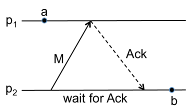
Figure 5: Synchronous message

Our timestamping algorithm does not constrain the messages to be synchronous. Our approach has some similarities to [6, 7] and also some key differences. In our case, the timestamp contains $2c+2$ integer elements, where $c$ is the size of the vertex cover of the communication network formed by the processes. Thus, the timestamps contain more elements because we allow the flexibility of using asynchronous messages. A consequence of allowing asynchronous messages is that the $next$ field of our inline timestamp may need to be modified up to $c$ times as the execution progresses, where $c=|\mathcal{C}|$ is the size of the chosen vertex cover of the communication graph. When vertex cover size is $c$, the network can be decomposed into $c$ stars. However, our algorithm does not utilize the decomposition as such (but instead uses the knowledge of a cover set $\mathcal{C}$). On the other hand, the algorithm in [6, 7] explicitly uses the decomposition into triangle and stars.

The $next$ field in our timestamp for events outside $\mathcal{C}$ includes an index for the receive event of one message sent to each of the $c$ processes in the vertex cover. Thus, the $next$ field includes $c$ elements. On the other hand, the timestamps in [6, 7] include just 1 index that has functionality analogous to one of the $c$ elements in our $next$ field. This index in the timestamp in [6, 7] counts messages in a component of the edge decomposition, whereas in our case, the index counts number of events at a process. These distinctions are caused by the restriction of synchronous messages in [6, 7], and allowance for asynchronous messages in our scheme.

Causal memory [8, 17]:

The purpose of the timestamps used in the work on causal memory is to ensure causal consistency. There are close similarities between our timestamps and comparable objects maintained in some causal memory schemes [8, 17].

In Lazy Replication [8], a client-server architecture is used to implement causally consistent shared memory. Each server maintains a copy of the shared memory. Each client sends its updates and queries to one of the servers. A server that receives an update from one of the clients then propagates the update to the other servers. Each server maintains a vector clock: the $i$-th entry of the vector at the $j$-server essentially counts the number of updates propagated to the $j$-th server by the $i$-th server. Each client also maintains a similar vector: the $i$-th element of the client’s vector counts the number of updates propagated by the $i$-th server on which the client’s state depends. Additionally, when a client sends its update to the $j$-th server, the $j$-th element of the client’s vector is updated to the index of the client’s update at the $j$-th server. The client may potentially send the same update to multiple servers, say, $j$-th and $k$-th servers; in this case, the $j$-th and $k$-th elements of the client’s vector will be updated to the indices of the client’s updates at the respective servers. Finally, a server cannot process an update or a query from a client until the server’s vector clock is $\geq$ the vector at the client. The $\geq$ operator here performs an element wise comparison of the vector elements: vector $v\geq w$ only if each element of $v$ is $\geq$ the corresponding element of vector $w$. This comparison operation differs slightly from the way we compare analogous elements in our timestamps in partial order $>$ for inline timestamps, as defined towards the end of Section 4. In particular, recall condition (iv) of the partial order $<$ from Section 4. In condition (iv), it suffices to satisfy inequality for just one element of the $next$ array. This is in contrast to vector comparison used in Lazy Replication.

The mechanism used in SwiftCloud [17] is motivated by Lazy Replication [8], and has close similarities to the vectors in [8]. In SwiftCloud, if a client sends its update to multiple servers, then the indices returned by the servers are merged into the dependency vector maintained by the client (optionally, some of the returned indices may not be merged). Importantly, a server can only respond to future requests from the client provided that the server’s vector covers the client’s dependency vector.

Beyond some small differences in how the timestamp comparison is performed, the other difference between shared memory schemes above and our solution is that the above schemes rely on a set of servers through which the processes interact with each other. Thus, the communication network in their case is equivalent to a clique of servers to which the clients are connected. The size of the timestamps is a function of the number of servers. On the other hand, we allow arbitrary communication networks, with the size of the timestamps being a function of a vertex cover for the communication network. The vertex cover is not necessarily completely connected. Secondly, dependencies introduced through events happening at the servers (e.g., receipt of an update from a client) in the shared memory systems are not necessarily true dependencies. For instance, suppose that process $p_{0}$ propagates update to variable $x$ to replica R, then process $p_{1}$ propagates update to variable $y$ to replica R, and finally process $p_{2}$ reads updated value of $y$ from replica R. In the shared memory dependency tracking schemes above, the update of $x$ by $p_{0}$ would be treated as having happened-before the read by $p_{2}$. In reality, there is no such causal dependency. But the dependency is introduced artificially as a cost of reducing the timestamp size. On the other hand, in the message-passing context, if the communication network reflects the communication channels used by the processes, then no such artificial dependencies will arise. However, in the message-passing case as well, we can introduce artificial dependencies by disallowing the use of certain communication channels in order to decrease the vertex cover size. This was illustrated in Section 5 through the example in Figure 3.

Appendix E Implementation Issues

In the inline algorithm, recall that elements of the $next$ field of the timestamps of events at processes outside $\mathcal{C}$ may have to be modified as many as $c$ times, where $c$ is the size of the vertex cover chosen by the algorithm.

In particular, when a process $p_{i}\not\in\mathcal{C}$ sends a message to some process $p_{j}\in\mathcal{C}$ at some time $t$, the $j$-th element of $next$ field in $\tau(e)$ as well as $next[j]$ element for any prior event $f$ for which $\tau(f).next[j]=\infty$, is modified to equal to the index of the receive event at $p_{j}$ corresponding to the message sent at $e$. Before the modification can be made, there is a delay due to the wait for a control message from $p_{j}$ that will inform $p_{i}$ of this index. Any queries at time $\geq t$ for the timestamps of event $e$, and events such as $f$, should not return until the index is known. To implement this, when the message is sent at $e$, the $next[j]$ element of $e$ and $f$ can be set to $\perp$ to indicate an invalid value – when such an invalid value is found in $next$ field for an event, the query procedure will know that it must wait for the invalid value to be updated before the event’s timestamp can be returned.

Secondly, consider the set of events, $E_{m}^{i,j}$, at a process $p_{i}\not\in\mathcal{C}$ that occur between the $m$-th and $m+1$-th messages sent by $p_{i}$ to a process $p_{j}\in\mathcal{C}$. Observe that for all the events in $E_{m}^{i,j}$ the $next[j]$ element of their timestamps is identical. This fact can be exploited by process $p_{i}$ to make it easier to update the timestamps stored at $p_{i}$. In particular, for all the events in $E_{m}^{i,j}$, the $next[i]$ element of the timestamp can point to an identical memory location – modifying this location then modifies the $j$-th element of all these timestamps simultaneously.

Two other improvements can be made to the $next$ component of the timestamp:

• Reducing the size of the $next$ field: In our discussion so far we assume that the $next$ field of the timestamp of an event outside $\mathcal{C}$ includes one element per process in $\mathcal{C}$. However, it suffices for the $next$ field for timestamps at process $p_{i}\not\in\mathcal{C}$ to include an element for each neighbor of $p_{i}$ in $\mathcal{C}$. Since process $p_{i}\not\in\mathcal{C}$ never sends a message directly to any process $p_{j}\in\mathcal{C}$ such that $(p_{i},p_{j})\not\in{\mathcal{E}}$, the elements of $next$ corresponding to such $p_{j}$ in timestamps for events at $p_{i}$ will always remain $\infty$. Hence these elements can be safely removed from the $next$ field. Thus reduces the size of the $next$ field for events at process $p_{i}\not\in\mathcal{C}$ to the number of its neighbor processes (which are necessarily all in $\mathcal{C}$).

• Reducing the delay in computing the $next$ field elements: In the basic algorithm presented in Section 4, for an event $e$ at process $p_{i}\in\mathcal{C}$, the $j$-th element of the $next$ field cannot be computed (where $(p_{i},p_{j})\in{\mathcal{E}}$) until a message from $p_{i}$ (sent at $e$ or later) is received by $p_{j}$. The essential use of the $next[j]$ field is to learn the index of the earliest event at $p_{j}$ that is “directly” influenced by event $e$ (“directly” here means due to a message from $p_{i}$ to $p_{j}$).

  Now we suggest a potential alternative, illustrated in Figure 6. In Figure 6(a), both the elements of the $next$ field of event $e$ at $p_{3}$ are $\infty$. As shown in Figure 6(c), although $p_{3}$ does not send a message to $p_{1}$ at or after event $f$, event $f$ does influence event $g$ at process $p_{1}$. In this case, it would be acceptable if $next[1]$ element of $\tau(e)$ and $\tau(f)$ is set equal to 2 (because $g$ is the second event at $p_{1}$). However, for $p_{3}$ to be able to learn this event index, additional control information will have to be exchanged between the processes. The benefit of the optimization is that the $next$ elements are changed from $\infty$ to finite values earlier than the basic approach illustrated earlier, but potentially at the cost of greater control overhead. A detailed design of this solution is not yet developed.

  

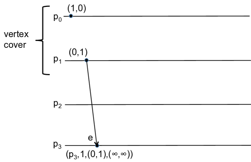
  (a)

  

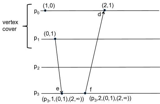
  (b)

  

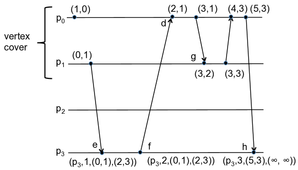
  (c)

  Figure 6: Improvement in $next$ computation

References

- [1] B. Charron-Bost. Concerning the size of logical clocks in distributed systems. Inf. Process. Lett., 39(1):11–16, 1991.
- [2] G. Coulouris, J. Dollimore, T. Kindberg, and G. Blair. Distributed Systems: Concepts and Design. Addison-Wesley Publishing Company, USA, 5th edition, 2011.
- [3] L. De Moura and N. Bjørner. Z3: An efficient smt solver. In Proceedings of the Theory and Practice of Software, 14th International Conference on Tools and Algorithms for the Construction and Analysis of Systems, TACAS’08/ETAPS’08, pages 337–340, Berlin, Heidelberg, 2008. Springer-Verlag.
- [4] C. J. Fidge. Logical time in distributed computing systems. IEEE Computer, 24(8):28–33, 1991.
- [5] V. K. Garg and C. Skawratananond. String realizers of posets with applications to distributed computing. In Proceedings of the Twentieth Annual ACM Symposium on Principles of Distributed Computing, PODC 2001, Newport, Rhode Island, USA, August 26-29, 2001, pages 72–80, 2001.
- [6] V. K. Garg and C. Skawratananond. Timestamping messages in synchronous computations. In ICDCS, pages 552–559, 2002.
- [7] V. K. Garg, C. Skawratananond, and N. Mittal. Timestamping messages and events in a distributed system using synchronous communication. Distributed Computing, 19(5-6):387–402, 2007.
- [8] R. Ladin, B. Liskov, L. Shrira, and S. Ghemawat. Providing high availability using lazy replication. ACM Trans. Comput. Syst., 10(4):360–391, 1992.
- [9] L. Lamport. Time, clocks and the ordering of events in a distributed system. Communications of the ACM, 21(7):558–565, July 1978.
- [10] F. Mattern. Virtual time and global states of distributed systems. In Parallel and Distributed Algorithms, pages 215–226. North-Holland, 1988.
- [11] S. Meldal, S. Sankar, and J. Vera. Exploiting locality in maintaining potential causality. In Proceedings of the Tenth Annual ACM Symposium on Principles of Distributed Computing, Montreal, Quebec, Canada, August 19-21, 1991, pages 231–239, 1991.
- [12] R. Schwarz and F. Mattern. Detecting causal relationships in distributed computations: In search of the holy grail. Distributed Computing, 7(3):149–174, 1994.
- [13] M. Shen, A. D. Kshemkalyani, and A. A. Khokhar. Detecting unstable conjunctive locality-aware predicates in large-scale systems. In IEEE 12th International Symposium on Parallel and Distributed Computing, ISPDC 2013, Bucharest, Romania, June 27-30, 2013, pages 127–134, 2013.
- [14] M. Singhal and A. D. Kshemkalyani. An efficient implementation of vector clocks. Inf. Process. Lett., 43(1):47–52, 1992.
- [15] F. J. Torres-Rojas and M. Ahamad. Plausible clocks: Constant size logical clocks for distributed systems. Distrib. Comput., 12(4):179–195, September 1999.
- [16] P. A. S. Ward and D. J. Taylor. Self-organizing hierarchical cluster timestamps. In Proceedings of the 7th International Euro-Par Conference Manchester on Parallel Processing, Euro-Par ’01, pages 46–56, London, UK, UK, 2001. Springer-Verlag.
- [17] M. Zawirski, N. Preguica, S. Duarte, A. Bieniusa, V. Balegas, and M. Shapiro. Write fast, read in the past: Causal consistency for client-side applications. In ACM Middleware, Vancouver, December 2015.