Radio variability in the Phoenix Deep Survey at 1.4GHz

Abstract

We use archival data from the Phoenix Deep Survey to investigate the variable radio source population above 1 $\mathrm{mJy}$/beam at 1.4 $\mathrm{GHz}$. Given the similarity of this survey to other such surveys we take the opportunity to investigate the conflicting results which have appeared in the literature. Two previous surveys for variability conducted with the Very Large Array (VLA) achieved a sensitivity of 1 $\mathrm{mJy}$/beam. However, one survey found an areal density of radio variables on timescales of decades that is a factor of $\sim 4$ times greater than a second survey which was conducted on timescales of less than a few years. In the Phoenix deep field we measure the density of variable radio sources to be $\rho=0.98\mathrm{deg}^{-2}$ on timescales of 6 months to 8 years. We make use of WISE infrared cross-ids, and identify all variable sources as an AGN of some description. We suggest that the discrepancy between previous VLA results is due to the different time scales probed by each of the surveys, and that radio variability at 1.4 $\mathrm{GHz}$ is greatest on timescales of $2-5$ years.

1 Introduction

There are many mechanisms which can cause variability in radio sources both intrinsic and extrinsic. Intrinsic variability can be due to variable accretion rates onto black holes, flare like activity in stars, tidal disruption events, or explosive events such as novae and supernovae. Extrinsic variability is typically induced either by scintillation due to turbulence in the interplanetary or interstellar medium (or the ionosphere at very low frequencies), or by extreme scattering events (Fiedler et al., 1994). Each of these mechanisms is understood, however the relative incidence and magnitude is less well understood.

The incidence of radio variability has been investigated with the aid of blind surveys using a combination of new and archival data. A common metric that is used to compare surveys with different attributes is the two epoch equivalent source density (Bower et al., 2007). Over time a trend has emerged: the more sensitive the survey detection limit, the greater the number of variable sources that are detected (Mooley et al., 2016). This trend is expected as the source count distribution of radio sources - there are more faint sources than bright sources. However there are many additional factors that contribute to differences in the density of variable radio sources including: observing frequency, observing cadence, integration time, and galactic latitude.

As the amount of intervening gas from the Milky Way’s interstellar medium (ISM) increases with lines of sight with lower Galactic latitudes, there is expected to be an increase in interstellar scintillation towards the Galactic plane. Gaensler & Hunstead (2000) found that there is a tendency for radio sources with $|b|<20\deg$ to be more likely to be variable, but that there was no correlation between the incidence, magnitude, or time-scale of variability above $|b|=20\deg$. This result is supported by Ofek & Frail (2011) who see a doubling in the fraction of variable sources below $|b|=20\deg$. Ghosh & Rao (1992) find an increase in the magnitude of variability at $10\deg<b<30\deg$ which is twice that at both higher and lower latitudes. At latitudes above $|b|=30\deg$ there is no indication that there is a relation between Galactic latitude and the incidence or magnitude of variability.

In the last decade considerable effort has been spent trying to map out the parameter space of radio variability. Much of this work has been focused around 1 $\mathrm{GHz}$ (see Mooley et al., 2016, and references there in), however studies at higher frequencies have also been done (eg, Bell et al., 2015; Bower et al., 2007). The studies at 1.4 $\mathrm{GHz}$ have spanned at least four orders of magnitude in sensitivity, giving a fairly sparse coverage of the parameter space. To date there have been only two blind surveys that have probed the same region of parameter space close enough to invite direct comparison, and they find a density of variable radio sources that differ by a factor of $\sim 4$. The first survey was conducted by Thyagarajan et al. (2011, hereafter T11), who compared the NVSS and FIRST survey images to search for radio variability, found variable sources with a density of $\rho=0.2\mathrm{deg}^{-2}$ above 1 $\mathrm{mJy}$/beam. The second survey was conducted by Hodge et al. (2013, hereafter H13), who compared multiple epochs of the FIRST survey and a new set of VLA observations, and found variable sources with a density of $\rho=0.74\mathrm{deg}^{-2}$ also above 1 $\mathrm{mJy}$/beam. The two surveys used the same telescope and frequency, had the same sensitivity, and both used data from the FIRST survey, and yet arrived at significantly different results. This discrepancy has not yet been explored in the literature. We therefore focus on the difference between the two surveys in order to explain the differing results.

In this paper we use archival data from the Phoenix Deep Survey to conduct a blind search for variable radio sources at 1.4 $\mathrm{GHz}$. The survey achieves a $5\sigma$ sensitivity of 1 $\mathrm{mJy}$/beam and can thus be used to understand the conflicting results of T11 and H13.

In section 2 we compare and contrast the T11 and H13 surveys and motivate the work of this paper. In section 3 we detail the data acquisition and reduction. In sections 4-5 we present the image and light curve analysis. We discuss the variables sources in section 6, and our results in section 7. We summarize and draw conclusions in section 8.

2 Survey comparison

T11 used data from the FIRST survey of the northern Galactic cap, covering nearly $8500\,\mathrm{deg}^{2}$. The survey area includes Galactic latitudes from $+17\deg$ to $+90\deg$, with 90% of the variable sources found above a latitude of $+30\deg$. H13 used data from the FIRST survey, and additional follow-up observations, to survey the SDSS stripe 82 region covering $60~{}\mathrm{deg}^{2}$. The area surveyed by H13 is restricted to a Galactic latitude of $40\deg<b<45\deg$. T11 and H13 survey different areas of sky but $>90\%$ of sources in these two surveys lie above $b=30\deg$. Since this is outside the $10\deg<b<20\deg$ enhancement region identified by (Ghosh & Rao, 1992) and others, Galactic latitude effects cannot be responsible for the different source densities observed.

Another difference between the T11 and H13 surveys is the time scales of variability that are probed. T11 worked with images that were separated by as little as 3 minutes up to a few years, with the majority of differences necessarily being at short time scales. H13 worked with three images each separated by 7 years. Thus T11 is more sensitive to short term variability, whilst H13 is sensitive only to long term variability on 7 year timescales. Ofek & Frail (2011) compared fluxes measured in the NVSS and FIRST surveys and showed that the amount of variability doesn’t change with observing cadences between $2-5$ years. In this work we use data with a cadence of between 150 and 2000 days, falling right between the peak sensitivity of the T11 and H13 surveys. In a study at 843 $\mathrm{MHz}$, Bannister et al. (2011) found some evidence that there is a peak in radio variability on timescales of between 2000 and 3000 days, which would suggest that the increased detection rate of H13 is a feature of the mechanism that is causing the radio variability.

The Phoenix Deep Survey microjansky catalog (PDS, Hopkins et al., 2003) was constructed from six epochs of data taken with the Australia Telescope Compact Array (ATCA) at 1.4 $\mathrm{GHz}$ over a period of 8 years. The mosaicked images from each epoch of observations achieve a sensitivity of $\sim 1$ $\mathrm{mJy}$/beam. We use the similarity between the frequency and sensitivity of these observations and the T11 and H13 observations, to investigate the conflicting results. The PDS data have a cadence that is between that of T11 and H13 and also covers the peak suggested by Bannister et al. (2011). We can therefore determine whether observing cadence plays an important role in the rate of variable sources that are observed in a given survey.

3 Data Acquisition and Reduction

We use archival observations of the PDS observed with the Australia Telescope Compact Array between 1993 and 2001 as part of the Phoenix Deep survey (PDS, Hopkins et al., 2003). The combined observations cover a $5.97$ $\mathrm{deg}^{-2}$ region of the sky at 1.4 GHz. The region is bound by 01:05:35$<$RA$<$01:22:22 and -47:01:59$<$Dec$<$-44:25:08.

Calibrated data were obtained from the PDS group. The calibration and imaging of these data are described in Hopkins et al. (1998), and Hopkins et al. (1999). As noted by Hopkins et al. (2003) the Phoenix field contains a number of bright sources that are difficult to clean completely and thus some mosaics contain artefacts around such sources. Since side-lobes and image artefacts can masquerade as variable or transient events, a second round of cleaning was performed around bright sources. This second round of cleaning significantly reduced the magnitude of the artefacts, however these artefacts still dominated the regions around bright sources. The data were grouped into six epochs, each with a duration of 1-22 days. Table 1 shows the observing dates, total imaged area, and median $5\sigma$ sensitivity, for each of the six epochs.

Observing	Name	Area	Sensitivity
Date(s)		($\mathrm{deg}^{2}$)	$5\sigma$(mJy)
28 Jan - 30 Jan 1994	1994E	3.79	2.29
3 Jul - 6 Jul 1994	1994L	4.50	1.82
27 Nov - 18 Dec 1997	1997	2.03	0.84
15 Sep 1999	1999	1.86	0.71
9 Sep- 13 Sep 2000	2000	2.62	0.69
1 Aug 2001	2001	1.59	0.76

Table 1: The observing dates, area, and median $5\sigma$ sensitivity of each epoch.

4 Image Analysis

We used the prototype pipeline developed for the Variables And Slow Transients (VAST, Murphy et al., 2013) survey (Banyer et al., 2012) to automate the source finding, crossmatching, and variability analysis. As part of the VAST pipeline, a mosaic of each epoch was processed using the Aegean source finding algorithm (Hancock et al., 2012).

4.1 Background and Noise characterization

Mooley et al. (2013) demonstrated that the Aegean source finding algorithm does not perform well in regions of an image where the background or noise is changing rapidly. The PDS field does not contain any significant diffuse background emission, however the noise in the mosaics increases around the edge of the image, and around bright sources. We use the Background And Noise Estimation program (BANE) to improve the completeness and reliability of the source finding in the presence of rapidly changing noise characteristics. BANE performs sigma clipping on the pixel distribution in order to provide a much more accurate measure of the background and noise properties of an image than the method used internally by Aegean. We did not follow the method of Hopkins (1998) who exclude regions of sky around bright sources.

4.2 Overlap Regions

The six epochs of observations do not all cover the same area of sky. There is a small area of sky of $0.28\,\mathrm{deg}^{2}$ that is imaged in all six epochs. To increase the area available to detect variable and transient sources we include all regions of sky that were observed in at least two epochs. Figure 1 shows the area of sky that is covered by between 1-6 epochs of observations, and Table 2 details the area, median sensitivity, and number of sources detected in each overlap region. When calculating the number of sources that are detected in each of the overlap regions ($N_{S}$), a correction is made to account for the reliability of each of the input images. For the remainder of this paper the number of sources in an epoch $(N_{S})$ indicates the number of sources detected that are expected to be real.

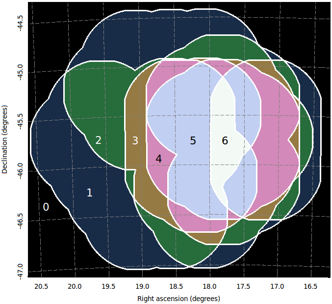
Figure 1: A representation of the overlap between each of the epochs considered in this work. Each shaded region represents between 1 to 6 images covering the given area of sky, as indicated by the annotations. The area of each region is listed in column 2 of Table 2.

Epochs	Area $=N_{E}$	$5\sigma$	Sources
($N_{E}$)	( $\mathrm{deg}^{2}$)	( $\mathrm{mJy}$/beam)	($N_{S}$)
1	2.09	3.35	336
2	1.19	2.48	410
3	0.50	1.58	453
4	0.83	0.97	498
5	1.08	0.61	594
6	0.28	0.72	328

Table 2: The area, median sensitivity, and source count, for the regions depicted in Figure 1. The source count ($N_{S}$) includes a correction for reliability.

5 Light Curve Analysis

The VAST pipeline produces three metrics for measuring the variability of a source, two metrics that measure the magnitude of variability and one metric that measures the significance of variability. The magnitude of variability is measured by the modulation index $m$ and the de–biased modulation index $m_{d}$ as described in Bell et al. (2014) (and references therein):

$$m =\frac{\bar{\sigma}_{s}}{\bar{S}}$$ (1a)

$$m_{d} =\frac{1}{\bar{S}}\sqrt{\frac{\sum^{n}_{i=1}\left(S_{i}-\bar{S}\right)^{2}-\sum^{n}_{i=1}\sigma_{i}^{2}}{n}},$$ (1b)

where $\bar{S},\bar{\sigma}_{s}$ are the mean and standard deviation of the fluxes in a light curve, $S_{i},\sigma_{i}$ are individual measurements within a light curve, and $n$ is the number of measurements. $m_{d}$ is taken to be negative when the discriminant of Eq 1b is negative.

To calculate the significance of variability we first measured the $\chi^{2}_{lc}$ for the light curve and computed the probability that the given value would be seen in a non-variable source. Following Bell et al. (2014) we calculated $\chi^{2}_{lc}$ as

$$\chi^{2}_{lc}=\sum^{n}_{i=1}\frac{(S_{i}-\bar{S})^{2}}{\sigma_{i}^{2}},$$ (2)

where $S_{i}$ is the $i$th flux density measurement with variance $\sigma_{i}^{2}$, and $\bar{S}$ is the weighted mean flux density. The significance of variability indicated by a particular $\chi^{2}_{lc}$ value is dependent on the number of points in the light curve. We therefore converted the $\chi^{2}_{lc}$ values into a probability that the given variation in the light curve is statistically insignificant given the errors on each flux measurement. This probability was calculated as the survival function for a $\chi^{2}$ distribution with $n-1$ degrees of freedom. The probability of variability was then converted to a significance level expressed in $\sigma$. This approach breaks the degeneracy between degree and significance of variability, which is not accounted for in early studies of variability, but is recently becoming more common (e.g, Bell et al., 2015). From the analysis above we identified 86 sources as being variable at the $3\sigma$ level.

Due to the large number of false positive detections in the individual epochs, each of the 86 candidate variable sources were manually inspected. The following criteria were used to identify sources that are not considered to be true variables:

1. the source is likely the side-lobe of a brighter source,

2. the source is a component of an extended or resolved source which is characterized by multiple components,

3. the source is only detected at the extreme edges of an image, or

4. the source is coincident with imaging artefacts that change between epochs.

After manual inspection all but 9 sources were eliminated from the sample of candidates. Of these 9 sources, 8 were detected in multiple epochs, whilst one was detected in only one epoch, and is thus classified as a transient source. These 9 sources are summarized in Table 3 and discussed in the following section.

ID	RA/Dec	PDS Flux	Modulation Index		Significance	Epochs	$\alpha_{0.843}^{1.4}$	Notes
	(J2000)	( $\mathrm{mJy}$/beam)	m	md	$\sigma$
Variable
A	01:08:21$-$45:28:32	$84.7\pm 0.9$	0.18	14.4	6.9	4/4	-1.3	SUMSS J010821-452835
B	01:09:53$-$46:31:29	$19.8\pm 0.2$	0.16	10.2	3.3	3/3	-1.2	SUMSS J010952-463130
C	01:10:14$-$46:15:07	$13.5\pm 0.2$	0.07	2.8	3.0	5/5	-2.2	SUMSS J011015-461502
D	01:11:14$-$45:36:01	$6.7\pm 0.1$	0.13	6.9	4.6	6/6	-1.0	SUMSS J011114-453555
E	01:12:17$-$46:29:32	$6.8\pm 0.1$	0.19	11.8	5.0	5/5	-
F	01:13:40$-$46:03:47	$15.7\pm 0.2$	0.09	5.4	7.4	5/5	-0.8	SUMSS J011341-460353
G	01:14:10$-$46:35:48	$48.7\pm 0.5$	0.08	3.9	4.9	3/3	-0.4	SUMSS J011410-463551
H	01:15:44$-$45:55:50	$39.8\pm 0.4$	0.11	6.5	$>$8	3/3	-0.8	SUMSS J011544-455549; z=0.104
Transient
T	01:13:35$-$46:11:13	$0.266\pm 0.044$	1.28	56.0	3.0	1/5	-

Table 3: The 8 variable sources and one transient source with a significance greater than $3\sigma$. The reported flux is taken from Hopkins et al. (2003), and is equal to a weighted sum of the flux of a source across all epochs. The modulation indexes m and m_d are calculated using equations 1a and 1b. The epochs column shows the number of epochs in which the source was detected and the total number of epochs in which the source could have been detected. The spectral index is taken between the PDS fluxes listed here and the corresponding measurement in the SUMSS catalog (where it exists, Mauch et al., 2003).

.

5.1 Variability

The areal density of variable sources ($\rho$) is calculated as:

$$\rho=\frac{\Sigma N_{V}}{\Sigma A(N_{E}-1)},$$ (3)

where $N_{V}$ is the number of variables, $N_{E}$ is the number of epochs in which the source was observed, and $A$ is the area of sky covered by $N_{E}$ epochs (see Figure 1). The summation is done over all overlap regions to obtain a single source density for this work. We use the above definition of variable source density throughout this paper. Mooley et al. (2016), and the associated online resource, was used as a reference for calculating all variable source densities quoted in this paper.

The fraction of sources that is variable is also calculated over all overlap regions, using:

$$V(\%)=\frac{\Sigma N_{V}}{\Sigma N_{S}},$$ (4)

where $N_{S}$ is the number of sources detected within the region of sky after correction for reliability. The mean sensitivity of the observation is weighted by the area of each overlap region via:

$$\bar{\sigma}=\frac{\Sigma\sigma A}{\Sigma A},$$ (5)

where $\sigma$ is the mean sensitivity listed in Table 2.

Using the above equations, the data in Table  3 represent an areal source density of variables of $\rho=0.86\,\mathrm{deg}^{-2}$, with a sensitivity of $\bar{\sigma}=1.4$ $\mathrm{mJy}$. The fractional of variable sources is $\sim 0.7\%$ at 1.4 $\mathrm{GHz}$ on timescales of 6 months to 8 years. This fraction is in agreement with that found by Mooley et al. (2013), at the same frequency but lower flux densities, in the extended Chandra deep field south. We therefore support the suggestion of Mooley et al. (2013), that the 1.4 $\mathrm{GHz}$ radio sky is relatively quiet.

5.2 Transients

One of the sources identified in Table 3 was detected in only a single epoch out of a possible five, and is thus a transient source. Using the same method as the previous section, we find a density of transients $\rho=0.1\,\mathrm{deg}^{-2}$ with a sensitivity of $\bar{\sigma}=1.4$ $\mathrm{mJy}$. Given a single transient source across all epochs, we estimate that in any image $0.1\%$ of all point sources above $1.4$ $\mathrm{mJy}$/beam will be a transient source. This density is consistent with an extrapolation from other studies at $1.4$ GHz (Mooley et al., 2013; Croft et al., 2010; Croft et al., 2011).

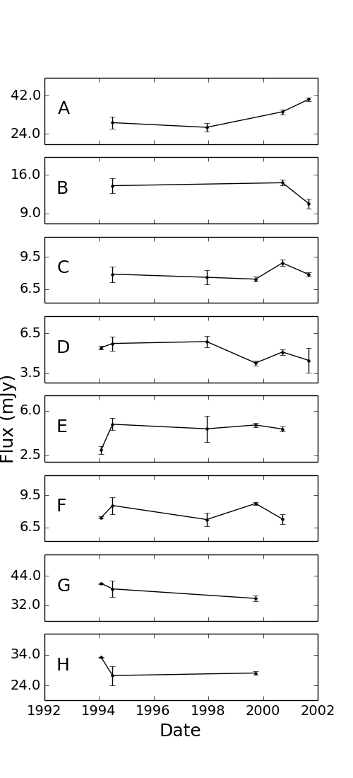
Figure 2: The light curves of variable sources A-H, scaled to emphasize the significance of variability. Error bars show $1\sigma$ uncertainties.

6 Variable Source Analysis

The light curves of all the variable sources are shown in Figure 2. The sparse sampling of these light curves precludes any indication of the cause of variability so we turn instead to multi-wavelength data to understand the nature of the sources and possibly the cause of variability.

Each of the sources were cross-matched with the SUMSS catalog (Mauch et al., 2003) and for all but sources E and T, a counterpart was found. The counterparts are all point sources and we calculate the average spectral index for each using the flux from the PDS and SUMSS catalogs. The spectral index of each source is shown in column 8 of Table 3. We note that the spectral indexes are all negative, which is in contrast to the positive spectral indexes that Bell et al. (2015) measured for variable sources found at 5 $\mathrm{GHz}$. Unlike the recent observations by Bell et al. (2015) the PDS observations were made prior to the ATCA broad-band upgrade, and so we are not able to extract an intra-band spectral index for any of the sources in our sample. A steep (or at least negative) spectral index is consistent with the optically thin spectrum of an AGN.

Comparing the variable sources to the Wide-field Infrared Survey Explorer (WISE, Wright et al., 2010) catalog we are able to obtain a cross identification for all sources. We place the sources on a color-color plot as shown in Figure 3. All the sources but two are consistent with an AGN of some description. Source C has colors that are consistent with either a star or elliptical galaxy, and source H is consistent with a spiral galaxy.

Sources A, C, and H were found to have matches in additional catalogs hosted by VizieR and are discussed in detail below, along with the transient source T.

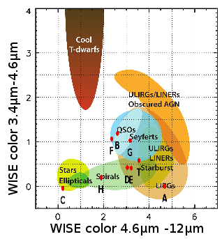
Figure 3: Each of the variable sources are identified according to their WISE colors. The red points are labeled according to the source ID, whilst the colored regions indicate the source classification. This image modified from Wright et al. (2010).

6.1 Source A

This is a previously known radio source that has been detected in a number of other radio surveys, as summarized in Table 4. The data are well described by a single power law with a spectral index of $\alpha=-0.77$. Source A is identified by Flesch (2010) as having an X-ray counterpart, and they assign a 93% probability that this source is a quasar. The spectral index of this source is consistent with an optically thin synchrotron emission. The variability that is observed could be due to intrinsic variability in the fueling of an AGN. With a de-biased modulation index of just 14.4 over a timescale of less than 8 years, intrinsic variability is certainly possible.

Frequency	Flux	Reference
GHz	mJy
0.180	$588\pm 73$	MWACS; Hurley-Walker et al. (2014)
0.843	$160\pm 0.49$	SUMSS; Mauch et al. (2003)
1.4	$84.7\pm 0.9$	PDS; Hopkins (1998)
4.8	$49\pm 10$	PMN; Gregory et al. (1994)

Table 4: The flux of source A as measured in multiple radio surveys. The data are well described by a single power law with spectral index of $\alpha=-0.77$.

6.2 Source C

Afonso et al. (2005) identify this source as a star with an r-magnitude of 14.89. This designation is consistent with the WISE colors seen in Figure 3. Source C appears in the XMM serendipitous source catalog (3XMM-DR4, Rosen et al., 2015) with a soft spectrum. The photon count in the XMM catalog is too low to obtain a secure classification using just the X-ray data. However when taken in combination the radio, infra-red and X-ray data for source C are consistent with a massive hot star with an unstable wind (Kudritzki & Puls, 2000).

6.3 Source H

The infrared colors of this source indicate that the host galaxy is a spiral (Figure 3). Afonso et al. (2005) observed this source as part of the PDS follow up and reported a redshift of $z=0.104$ with a spectrum that indicates star-formation and narrow emission-line system. Afonso et al. (2005) also report a $H_{\alpha}$ luminosity of $10^{34.83}W$ and 1.4 $\mathrm{GHz}$ luminosity of $10^{24.3}W\,Hz^{-1}$, making it the most radio luminous of all the star-forming galaxies identified in the follow up observations. Variability in a galaxy with star formation indicates that there are multiple sources of emission, with only the compact component being variable. Narrow emission lines are common but not exclusive to in AGN, however the presence of radio variability is evidence for an AGN core. We conclude that this source is an AGN with active star-formation.

6.4 Source T

As mentioned in the previous section, source T was identified in the variability search and was detected in only a single epoch out of a total of five observations. The flux at the location of the transient was measured in the remaining four observations. In three epochs (1994E, 1997, 2000) the measurements is consistent with zero flux, however in epoch 1994L the measurement indicates a source with a non-zero flux but at the $2\sigma$ level. Figure 4 shows the light curve for the transient source, along with a sequence of images from each of the five epochs of observations.

The 1999 epoch detection is $12.8$ times the local rms, making this single detection highly significant, even though the significance of the variability is only $3\sigma$. The PDS catalog lists the flux of this source as being $0.266\pm 0.044$ $\mathrm{mJy}$, whilst the 1999 epoch detection is at a flux of $0.314\pm 0.034$ $\mathrm{mJy}$. This agreement in flux is due to the fact that at the location of source T the 1999 image has a very small local noise ($0.025$ $\mathrm{mJy}$/beam), where as the other epochs have a local rms that is 3-5 times greater. The linear mosaicking that was used by Hopkins (1998) used a weighting scheme that was proportional to the inverse square of the local rms and thus the signal from the 1999 epoch dominates the flux measurement.

The fact that source T has a low significance detection in the 1994L epoch suggests that the source may have some amount of quiescent emission. It is possible that we are seeing a faint AGN that is undergoing interstellar scintillation and that in the 1999 epoch scintillation has boosted the flux of the source to a detectable level. If this is the case then source T would have a light curve more similar to the variable sources that have been previously discussed. An infrared counterpart was detected for this source, and the counterpart has colors consistent with an AGN (see Figure 3). The light-curve and the designation as an AGN means that although this sources was detected as a transient we consider this to be a variable source at the edge of our detection limit. If we consider this source to be a variable rather than a transient, then we arrive at a revised source density of $\rho=0.98\,\mathrm{deg}^{-2}$ for variables, and an upper limit of $<0.1\,\mathrm{deg}^{-1}$ for transients.

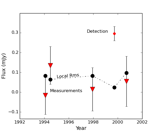
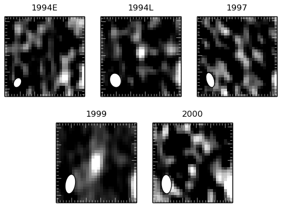
Figure 4: Upper: The light curve for the transient source T. The single detection is the highest labeled point, and the triangular points show the measurements in the remaining epochs. The dot-dashed line and points indicated the $1\sigma$ local noise at each epoch. Lower: Images centered on the location of the transient (01:13:35$-$46:11:13) for each of the five epochs that covered this region of sky. The white ellipse is the size of the synthesized beam, and the images are 0$\aas@@fstack{\prime}$48 on a side.

7 Discussion

Figure 5 compares the areal source density found in this work to that of other radio variability studies at $\sim 1$ GHz. In compiling data for Figure 5, we consider only blind radio surveys for variability at frequencies between 0.5 and 2 GHz. The timescales of variability that are probed by the various studies are also shown in Figure 5, for comparison. If we consider all the 9 sources identified in the previous section as variables, then we measure a variable areal source density of $\rho=0.98\mathrm{deg}^{-2}$. If we look at surveys with a sensitivity of $\sim 1$ $\mathrm{mJy}$/beam we have: Frail et al. (1994) ($\rho=0.076\,\mathrm{deg}^{-2}$) on timescales of days to months, T11 ($\rho=0.2\,\mathrm{deg}^{-2}$) on timescales of minutes to years, this work on timescales of 6 months to 8 years, and finally H13 ($\rho=0.74\mathrm{deg}^{-2}$) on timescales of $7-14$ years. There is a common story unfolding here: surveys with a cadence of years-decades detect more variable sources than those with a cadence of days-months. It should be noted that the work of Croft et al. (2010) probed the longest time scales of all the surveys in Figure 5, but found a source density that is the lowest of all. This would suggest that the relationship between observing cadence and variable source density is not monotonic. Both the increase of variability on longer timescales, and the decrease at the longest timescales is consistent with the suggestion of Bannister et al. (2011) that variability is greatest on timescales of $\sim 2-5$ yr.

A peak in the variability of radio sources as a function of observing cadence is in disagreement with the work of Ofek & Frail (2011) who measure a structure function of variability is flat. However Ofek & Frail (2011) rely on data that spanned timescales of 1 month to 5 years which is both longer than the shortest timescales accessible to T11, and shorter than the shortest timescales probed by H13. Despite this disagreement on the incidence of variability, we agree with Ofek & Frail (2011) on the primary cause of variability - interstellar scintillation of a compact component making up at least a fraction of the flux observed in each of the sources.

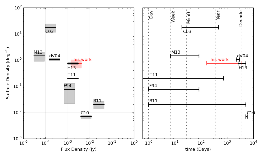
Figure 5: Two epoch equivalent areal density of variable sources detected at 1.4GHz. Left: Source density as a function of flux density. Shaded boxes represent Poisson errors on the number of detected variable sources. Right: The timescales probed by the surveys indicated in the left panel. The variables found within the phoenix field have an areal density that agrees with that measured by H13. The range of timescales probed by this work bridges a gap between the timescales probed by previous surveys. References are: C03 - (Carilli et al., 2003), M13 - (Mooley et al., 2013), dV04 - (de Vries et al., 2004), H13 - (Hodge et al., 2013), F94 - (Frail et al., 1994), C10 - (Croft et al., 2010), B11 - (Bannister et al., 2011), T11 - (Thyagarajan et al., 2011), and this work.

Of the 9 identified sources, all but one have a counterpart in the SUMSS survey and a negative spectral index. These spectral indexes are consistent with classical AGN in the optically thin regime. If we consider intrinsic variability with an AGN then we would expect the light curve to be a superposition of self absorbed SEDs each cooling and passing through the observing band. Thus the spectral index would be positive and negative for approximately equal amounts of time. In our snapshot of 9 sources we find only negative spectral indexes which argues against such a model of intrinsic variability. Alternatively, we suggest that the variability that we are primarily observing is interstellar scintillation of AGN (Ofek & Frail, 2011).

Source C is a notable exception to the above arguments in that it is not an AGN. In this case the emission is coming from shocks in the wind of a hot star (Kudritzki & Puls, 2000), on scales much less than a light year. Intrinsic variability on timescales of years has been seen before in such objects (eg, van Loo et al., 2008) and is thus a possible explanation.

For extragalactic radio sources, we find that radio variability is dominated by interstellar scintillation. The scintillating medium is necessarily of Galactic origin. Investigations into long-term radio variability at $\sim 1\,\mathrm{GHz}$ frequencies tell us less about the observed sources, and more about the nature of gas within our own Galaxy. This focus is contrary to the stated goals of many radio variability surveys. Future radio surveys which aim to explore a new parameter space of transient and variable objects, with a focus on intrinsic variability, should thus focus attention on short timescales (and thus explosive events). However, long-time scale variability studies can offer a new insight into the distribution and behavior of gas within the Milky Way.

8 Summary and Conclusions

We used six epochs of data from the Phoenix Deep Survey to search for variables and resolve the conflict between the results of Thyagarajan et al. (2011) and Hodge et al. (2013). We measure the density of variable radio sources to be $\rho=0.98\mathrm{deg}^{-2}$ which is consistent with that of Hodge et al. (2013). Given the overlap in timescales probed by this work that and that of Hodge et al. (2013), and the shorter timescales probed by Thyagarajan et al. (2011), we suggest that the discrepancy in variable source density could be due to the different time scales that were probed.

We have made use of infrared colors from the WISE survey to provide a fast identification of source types, and fond that all variable sources are consistent with an AGN. This approach is likely to find continued use in large area transient and variable surveys, where automated host typing will allow for more appropriate follow up observations. This will be particularly important for the search for hosts of Fast Radio Bursts and Gravitational Wave events.

Eight of the nine variable sources detected in this work show behavior consistent with interstellar scintillation of AGN, whilst the remaining source shows variability that can be attributed to intrinsic causes. Our results support the claim of Bannister et al. (2011), that variability at $\sim 1\,\mathrm{GHz}$ frequencies is greatest on timescales of $2-5$ years.

References

- Afonso et al. (2005) Afonso J., Georgakakis A., Almeida C., Hopkins A. M., Cram L. E., Mobasher B., Sullivan M., 2005, The Astrophysical Journal, 624, 135
- Bannister et al. (2011) Bannister K. W., Murphy T., Gaensler B. M., Hunstead R. W., Chatterjee S., 2011, Monthly Notices of the Royal Astronomical Society, 412, 634
- Banyer et al. (2012) Banyer J., Murphy T., VAST Collaboration 2012, in Ballester P., Egret D., Lorente N. P. F., eds, Astronomical Society of the Pacific Conference Series Vol. 461, Astronomical Data Analysis Software and Systems XXI. p. 725
- Bell et al. (2015) Bell M. E., Huynh M. T., Hancock P., Murphy T., Gaensler B. M., Burlon D., Trott C., Bannister K., 2015, Monthly Notices of the Royal Astronomical Society, 450, 4221
- Bell et al. (2014) Bell M. E. et al., 2014, Monthly Notices of the Royal Astronomical Society, 438, 352
- Bower et al. (2007) Bower G. C., Saul D., Bloom J. S., Bolatto A., Filippenko A. V., Foley R. J., Perley D., 2007, The Astrophysical Journal, 666, 346
- Carilli et al. (2003) Carilli C. L., Ivison R. J., Frail D. A., 2003, The Astrophysical Journal, 590, 192
- Croft et al. (2010) Croft S. et al., 2010, The Astrophysical Journal, 719, 45
- Croft et al. (2011) Croft S., Bower G. C., Keating G., Law C., Whysong D., Williams P. K. G., Wright M., 2011, The Astrophysical Journal, 731, 34
- de Vries et al. (2004) de Vries W. H., Becker R. H., White R. L., Helfand D. J., 2004, The Astrophysical Journal, 127, 2565
- Fiedler et al. (1994) Fiedler R., Dennison B., Johnston K. J., Waltman E. B., Simon R. S., 1994, The Astrophysical Journal, 430, 581
- Flesch (2010) Flesch E., 2010, Publications of the Astronomical Society of Australia, 27, 283
- Frail et al. (1994) Frail D. A. et al., 1994, The Astrophysical Journal Letters, 437, L43
- Gaensler & Hunstead (2000) Gaensler B. M., Hunstead R. W., 2000, Publications of the Astronomical Society of Australia, 17, 72
- Ghosh & Rao (1992) Ghosh T., Rao A. P., 1992, Astronomy and Astrophysics, 264, 203
- Gregory et al. (1994) Gregory P. C., Vavasour J. D., Scott W. K., Condon J. J., 1994, Astrophysical Journal Supplement Series, 90, 173
- Hancock et al. (2012) Hancock P. J., Murphy T., Gaensler B. M., Hopkins A., Curran J. R., 2012, Monthly Notices of the Royal Astronomical Society, 422, 1812
- Hodge et al. (2013) Hodge J. A., Becker R. H., White R. L., Richards G. T., 2013, The Astrophysical Journal, 769, 125
- Hopkins et al. (1999) Hopkins A., Afonso J., Cram L., Mobasher B., 1999, The Astrophysical Journal, 519, L59
- Hopkins (1998) Hopkins A. M., 1998, PhD thesis, School of Physics, University of Sydney, NSW, 2006, Australia
- Hopkins et al. (2003) Hopkins A. M., Afonso J., Chan B., Cram L. E., Georgakakis A., Mobasher B., 2003, The Astronomical Journal, 125, 465
- Hopkins et al. (1998) Hopkins A. M., Mobasher B., Cram L., Rowan-Robinson M., 1998, Monthly Notices of the Royal Astronomical Society, 296, 839
- Hurley-Walker et al. (2014) Hurley-Walker N. et al., 2014, Publications of the Astronomical Society of Australia, 31, e045
- Kudritzki & Puls (2000) Kudritzki R.-P., Puls J., 2000, Annual Review of Astronomy and Astrophysics, 38, 613
- Mauch et al. (2003) Mauch T., Murphy T., Buttery H. J., Curran J., Hunstead R. W., Piestrzynski B., Robertson J. G., Sadler E. M., 2003, Monthly Notices of the Royal Astronomical Society, 342, 1117
- Mooley et al. (2013) Mooley K. P., Frail D. A., Ofek E. O., Miller N. A., Kulkarni S. R., Horesh A., 2013, The Astrophysical Journal, 768, 165
- Mooley et al. (2016) Mooley K. P. et al., 2016, The Astrophysical Journal, 818, 105
- Murphy et al. (2013) Murphy T. et al., 2013, Publications of the Astronomical Society of Australia, 30, 6
- Ofek & Frail (2011) Ofek E. O., Frail D. A., 2011, The Astrophysical Journal, 737, 45
- Rosen et al. (2015) Rosen S. et al., 2015, in Taylor A. R., Rosolowsky E., eds, Astronomical Society of the Pacific Conference Series Vol. 495, Astronomical Data Analysis Software an Systems XXIV (ADASS XXIV). p. 319
- Thyagarajan et al. (2011) Thyagarajan N., Helfand D. J., White R. L., Becker R. H., 2011, The Astrophysical Journal, 742, 49
- van Loo et al. (2008) van Loo S., Blomme R., Dougherty S. M., Runacres M. C., 2008, Astronomy and Astrophysics, 483, 585
- Wright et al. (2010) Wright E. L. et al., 2010, The Astronomical Journal, 140, 1868