Abstract

A good clustering can help a data analyst to explore and understand a data set, but what constitutes a good clustering may depend on domain-specific and application-specific criteria. These criteria can be difficult to formalize, even when it is easy for an analyst to know a good clustering when they see one. We present a new approach to interactive clustering for data exploration called TINDER, based on a particularly simple feedback mechanism, in which an analyst can reject a given clustering and request a new one, which is chosen to be different from the previous clustering while fitting the data well. We formalize this interaction in a Bayesian framework as a method for prior elicitation, in which each different clustering is produced by a prior distribution that is modified to discourage previously rejected clusterings. We show that TINDER successfully produces a diverse set of clusterings, each of equivalent quality, that are much more diverse than would be obtained by randomized restarts.

1 Introduction

Clustering is a popular tool for exploratory data analysis. Good clusterings can help to guide the analyst to better understandings of the dataset at hand. What constitutes a good, informative clustering is not just a property of the data itself but also needs to capture the overall goals of the analyst. What makes it challenging to identify a good clustering is that it is often difficult to encode the analyst’s goals explicitly as machine learning objectives. Moreover, in many settings, the analyst does not have a well-specified objective in mind prior to encountering the data, but rather continuously updates her goals as she learns more through exploratory analysis.

The design of a clustering algorithm necessarily reflects prior assumptions about what types of clusters are meaningful. For example, these assumptions manifest in the distance metric for a $k$-means clustering algorithm or the choice of the prior distribution and likelihood when clustering using a probabilistic model. This raises an obvious chicken and egg problem: exploration via clustering is a major tool for helping an analyst learn about a data set, but such exploration is likely to influence their opinion about what types of clusters would be meaningful.

Put another way: because the clustering problem is ill-posed, many equivalently (quantitatively) good clusterings exist for a given data set. Even if a clustering algorithm succeeds in finding a (quantitatively) good clustering, it still may not be what the user (qualitatively) wanted. Nevertheless, the data analyst may not be able to formalize precisely as a quantitative criterion what differentiates a “good” clustering from a “bad” one. Still, it seems reasonable to expect that the analyst will know a good clustering when they see one.

This gap between formal clustering criteria and the user’s exploratory intuition is the motivation for interactive and alternate clustering approaches. Interactive clustering approaches present the user with an initial clustering, upon which the analyst can provide feedback and induce the system to modify the clustering. Several different types of interaction are described in this literature: the analyst can request that whole clusters be split or merged Cutting et al. (1992); Balcan & Blum (2008), that pairs of data points either must be linked or should not be linked in one cluster Wagstaff et al. (2001), or that the clustering should focus only on a subset of features Bekkerman et al. (2007). Although all of these modes of interaction can be useful in certain data analytic settings, they require to a greater or lesser degree that the analyst have a sense of how the initial clustering can be improved. Sometimes this may be clear, but we suggest that there are other situations in which the analyst can tell that a clustering does not meet their exploratory needs, without having a clear idea of how it should be improved.

In contrast, alternative clustering methods Gondek & Hofmann (2004); Bae & Bailey (2006); Caruana et al. (2006); Jain et al. (2008); Dang & Bailey (2010); Cui et al. (2010) focus on generating a set of high-quality clusterings that are chosen to be different from each other, which the user can select between. Work in this area has generated diverse sets of clusters by randomly reweighting features Caruana et al. (2006), by exploring the space of possible clusterings using Markov Chain Monte Carlo Cui et al. (2010), or by penalizing the objective function to encourage clusterings to be diverse Gondek & Hofmann (2004); Jain et al. (2008); Dang & Bailey (2010). Our framework for interactive clustering includes alternative clustering as a special case, bridging between interactive and alternative clustering.

To allow the user to provide “non-constructive” feedback on a clustering, we introduce a simple rejection-based approach to interactive clustering, in which the analyst rejects a given clustering and requests a different one. The system returns another clustering, which is chosen to be as different as possible from the previous clustering, while still fitting the data well according to a standard quantitative criterion. To reflect the notion of “rejecting” a clustering, we call this interaction mechanism TINDER (Technique for INteractive Data Exploration via Rejection).

2 Interactive Clustering

Now we describe the rejection-based framework for interactive clustering. We begin with an overview of the interaction method. The data are first clustered according to a standard clustering algorithm. We present this clustering to the analyst for inspection, for example, by displaying the data points or the features that are most closely associated with each cluster. Then the analyst has two options: if the clustering meets the information need of the analyst, then they can explore the data set accordingly. Otherwise the analyst tells the algorithm to reject the clustering and present a different one. If the clustering is rejected, we cluster the data again, modifying the objective function for the clustering algorithm to penalize clusterings that are similar to the previous one. This is to encourage returning a new clustering which is as different as possible from the previous one, but that still fits the data well according to the quantitative objective function of the original clustering algorithm.

This new clustering is then presented to the user, and this process can be repeated as many times as desired. We call each iteration of this process a feedback iteration. That is, the clustering in feedback iteration 0 is simply the standard clustering returned by the clustering algorithm without any feedback, the clustering from feedback iteration 1 incorporates a penalty so that it is different from clustering 0, and so on. When computing the clustering from the second and subsequent feedback iterations, we include penalty terms to encourage the new clustering to be different from all previous clusterings that the analyst has seen, so that the clusterings do not oscillate.

In a Bayesian setting, this interaction mechanism can be formalized naturally as a type of prior elicitation. At each feedback iteration $t$, we perform Bayesian clustering with parameters $\theta$, but with a different prior $\pi_{t}(\theta)$ that strongly downweights parameter vectors that would result in clusterings similar to previous ones. More formally, given a data set $\mathbf{x}=(x_{1},\ldots x_{n})$, we obtain the initial clustering for feedback iteration 0 using a standard Bayesian mixture model

$$p_{0}(x,\theta)=\sum_{h}p(x|h,\theta)p(h|\theta)\pi_{0}(\theta),$$ (1)

where we are using the subscript $0$ to indicate the feedback iteration. For computational reasons, we perform maximum a posteriori (MAP) estimation of $\theta$, resulting in a point estimate $\theta_{0}$ of the parameters. Let $\mathbf{h}=(h_{1}\ldots h_{n})$ denote a cluster assignment for each of the data points, so that after MAP estimation we have a soft assignment $p(\mathbf{h}|\mathbf{x},\theta_{0})$ over the cluster labels of all data points. (Notice that this distribution is not a function of the prior $\pi_{0}(\theta)$, so we do not subscript $p$ with the feedback iteration.)

This clustering is displayed to the user, who can then offer feedback, either accepting or rejecting the clustering.

Supposing that the clustering is rejected, working within a Bayesian framework, we interpret this feedback as a new, indirect source of information about the analyst’s prior beliefs over $\theta,$ but which they were unable to encode mathematically into the prior distributions used in the previous feedback iterations. Therefore, to cluster the data during feedback iteration $t$, we define a revised prior distribution $\pi_{t}(\theta)$ and perform MAP estimation again to obtain a new parameter estimate $\theta_{t}$. The prior $\pi_{t}$ is designed in such a way that when we consider the resulting soft assignment over cluster labels, which we denote $p(\mathbf{h}|\mathbf{x},\theta_{t}),$ this clustering will be as different as possible from the clusterings $p(\mathbf{h}|\mathbf{x},\theta_{0})\ldots p(\mathbf{h}|\mathbf{x},\theta_{t-1})$ at all previous feedback iterations.

Now we describe the form of the prior $\pi_{t}(\theta)$ that we use at feedback iteration $t$. We define the prior to have the form

$$\pi_{t}(\theta)\propto\pi_{0}(\theta)\prod_{s=0}^{t-1}\exp\{-\beta f(\theta,\theta_{s})\},$$

where $f$ is a function that measures the degree of similarity between the cluster distribution $p(\mathbf{h}|\mathbf{x},\theta)$ and the distribution $p(\mathbf{h}|\mathbf{x},\theta_{s})$ that the user rejected after feedback iteration $s$. The parameter $\beta$ is a temperature parameter.

A naive choice for $f(\theta,\theta^{\prime})$ would be to use the negative Kullback-Leibler divergence between the distributions $p(h|\theta)$ and $p(h^{\prime}|\theta^{\prime})$. However, in the context of clustering, this metric suffers from the issue of label switching, i.e., merely permuting the cluster assignments can produce high divergence. Instead, given two parameter settings $\theta$ and $\theta^{\prime}$, we begin by defining a joint distribution over the two corresponding cluster labels $h$ and $h^{\prime}$ as

$$p_{\theta,\theta^{\prime}}(h,h^{\prime},x)=p(h|x,\theta)p(h^{\prime}|x,\theta^{\prime})\tilde{p}(x),$$ (2)

where $\tilde{p}(x)=N^{-1}\sum_{i}\delta_{x,x_{i}}$ is the empirical distribution over data points, for the Kronecker delta function $\delta.$

Now $p_{\theta,\theta^{\prime}}$ is the joint distribution that results from randomly choosing a data item $x$, and clustering it independently according to the distributions $p(h|x,\theta)$ and $p(h^{\prime}|x,\theta^{\prime})$. This now defines a bivariate marginal distribution

$$p_{\theta,\theta^{\prime}}(h,h^{\prime}) =\sum_{x}p_{\theta,\theta^{\prime}}(h^{\prime},h,x)$$

$$=\frac{1}{N}\sum_{j=1}^{N}p(h_{j}|x_{j},\theta)p(h^{\prime}_{j}|x_{j},\theta^{\prime})$$ (3)

that measures the dependence between the two different clusterings, marginalizing out the data.

We define our metric to be the mutual information between the two random variables $H$ and $H^{\prime}$ whose distribution is given by $p_{\theta,\theta^{\prime}}(h,h^{\prime}).$ This yields

$$f(\theta,\theta^{\prime})=I(H;H^{\prime}) =\sum_{h,h^{\prime}}p_{\theta,\theta^{\prime}}(h,h^{\prime})\log\frac{p_{\theta,\theta^{\prime}}(h,h^{\prime})}{p_{\theta}(h)p_{\theta^{\prime}}(h^{\prime})}.$$

We note that because $f(\theta,\theta^{\prime})\geq 0$, we have that $\pi_{t}$ will be a proper prior if $\pi_{0}$ is. This completes the definition of the model. MAP estimation on this model is equivalent to maximizing

$$L_{t}(\theta)=\sum_{i}\log p_{\theta}(x_{i})-\beta\sum_{s=1}^{t-1}f(\theta,\theta_{s})+\log\pi_{0}(\theta),$$ (4)

where the temperature parameter $\beta$ now acts as a weighting parameter to bring the terms to a common scale.

2.1 Illustrative Example

Consider the task of clustering a synthetic 2-D dataset shown in figure 1 (a), which is generated from a mixture of four isometric Gaussians. The ellipses in (a) show the clustering resulting by maximizing the likelihood of a mixture of two gaussians using EM in the zeroth feedback iteration of TINDER. Starting from here, (b) shows an alternative clustering that TINDER generates in the next feedback iteration. Running another feedback iteration from (b) produces (c). Therefore using TINDER, an analyst can obtain three quantitatively different explanations for their data by running just three feedback iterations.

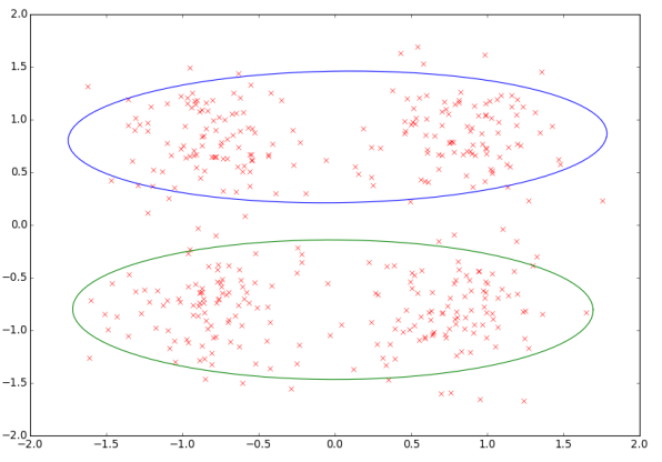
(a)

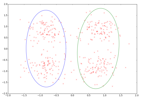
(b)

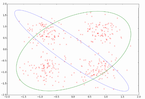
(c)

Figure 1: Example of TINDER clusterings produced in three feedback iterations on synthetic data generated by a mixture of 4, 2D, isometric Gaussians with $\beta=1$.

3 Experiments

We tested our method on a large collection of 10,000 thumbnail images from CIFAR 10 Krizhevsky & Hinton (2009). For evaluation of clustering diversity Adjusted Rand Score (ARS) and Normalized Mutual Information (NMI) are used; for both metrics, larger values indicate that the two clusterings being compared are more divergent. The cluster purity measure is used for measuring the classification accuracy.

3.1 Experiment Methodology

We use a mixture of gaussians model for the dataset and for the zeroth feedback iteration we set $\pi_{0}(\theta)$ to be one. We tested the model for different settings for the desired number of clusters, $K\in\{5,10,15,20,25\}$ and found that the diversity results were the same. Therefore, we show the results for $K=10$ only, also because for CIFAR10 this is equal to the actual number of clusters in the ground truth. In the previous section we introduced a weighting parameter $\beta$ on the prior. This is necessary as the likelihood and mutual information based prior are not on the same scale. Empirically, we found that TINDER performs well by simply setting $\beta$ such that the penalty term, $\beta\sum_{s}f$, and the log-likelihood have the same order of magnitude.

3.2 Results

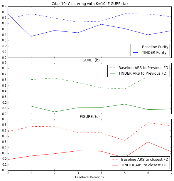
Figure 2: Comparision of the diversity and accuracy of the clusterings produced by TINDER and the baseline method on CIFAR10 for $\beta=1000$.

TINDER is able to produce a set of highly diverse and reasonably accurate clusterings on the CIFAR10 dataset as shown above. The middle plot in Figure 2 shows the diversity among all the pairs of consecutive clusterings for TINDER and the baseline method. It shows that the consecutive clusterings are far more diverse in the case of TINDER (solid green line) than the baseline (dashed green line). TINDER iteratively penalizes the likelihood function for all the previously produced clusterings in order to promote diversity in the upcoming results. Therefore any set of clusterings generated by TINDER is highly diverse with minimal overlap between all permutations of pairs. The bottom plot shows how the overall diversity of the set of clusterings in both the methods compares with each other. The solid red line plots for every clustering in the set produced by TINDER, the ARS to the closest clustering in the set or the maximum of all the pairwise ARS score in the set. Clearly, TINDER is consistently able to produce a highly diverse set of clusterings. Compared to this, the baseline method (dashed red line) does far worse with almost 50% or more overlap between all pair of clusterings. The top plot in Figure 2 shows the purity of the clusterings generated by the two methods. Notice that there is drop in the purity score of TINDER clusterings compared to the baseline method. TINDER is able to systematically explore the clustering space, by trading off the quality of the clustering–measured in terms of purity–with the desire to have clusterings that are sufficiently different from the rejected versions.

It is worth mentioning that by choosing the temperature parameter $\beta$ appropriately TINDER can be used for fine tuning the previous clusterings to arrive at better ones. The results on the NMI scale are practically the same as for ARS and therefore we do not report them here.

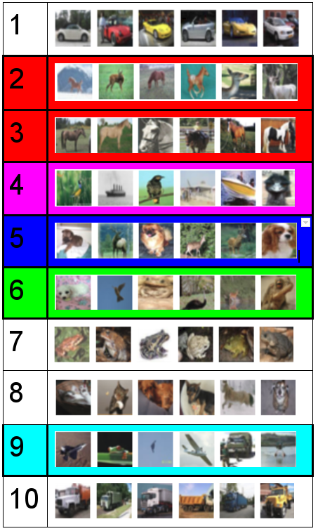
(a) Clustering 0 (no feedback)

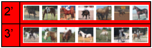
(b) Clustering 1 (after one feedback iteration). For space, only two of the ten clusters are shown.

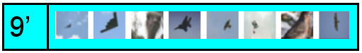
(c) Clustering 2 (after two feedback iterations). For space, only one of the ten clusters is shown.

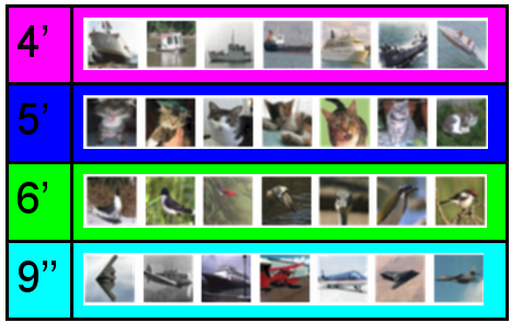
(d) Clustering 5 (after five feedback iterations). For space, only four of the ten clusters are shown.

Figure 3: Example of TINDER clusterings on CIFAR10 dataset.

To illustrate the effect of the feedback, we display in Figure 3 some of the clusters from TINDER on the CIFAR10 dataset. TINDER clusterings are not just able to find all the original CIFAR10 clusters but other meaningful clusters as well. In the figure, each of the rows represents a cluster and shows the top 6 images from that cluster ordered by their likelihood under the cluster. Figure 3(a) shows the initial clustering for $K=10$ with no feedback. Clustering 1 (Figure 3(b)) is produced by TINDER after a single iteration of feedback. We see that Clusters 2 and 3 from Clustering 0 (which contain deer and horses, respectively) are replaced in Clustering 1 by clusters 2’ and 3’, which contain large animals (Cluster 2’) and horses with riders (Cluster 3’). The result of the next feedback iteration is shown in Clustering 2 (Figure 3(c)). We see that Cluster 9 has been replaced by Cluster 9’, which contains images of birds and planes, which were scattered over multiple clusters in Clustering 0. Finally, after five feedback iterations, Clustering 5 (Figure 3(d)) includes clusters of ships (Cluster 4’), cats (Cluster 5’), birds (Cluster 6’) and planes (Cluster 9”), which did not exist in Clustering 0. These new clusters replace Clusters 4-6 and 9 from Clustering 0, which have low purity.

4 Conclusion

In this paper we have presented a method for interactive clustering based on a particularly simple feedback mechanism, in which an analyst can simply reject a clustering and request a new one. The interaction is formalized as a method of prior elicitation in a Bayesian model of clustering. We showed the efficacy of this method on image dataset as compared to the baseline method of random restarts. A natural extension of the current work would be to allow cluster level interaction as well as to provide a comparative analysis with alternate clustering methods. Another interesting direction of future work would be to extend the approach here to other unsupervised data-exploration models, where we can iteratively incorporate user feedback into priors.

References

- Bae & Bailey (2006) Bae, E. and Bailey, J. COALA: A novel approach for the extraction of an alternate clustering of high quality and high dissimilarity. In IEEE International Conference on Data Mining (ICDM), pp. 53–62, 2006.
- Balcan & Blum (2008) Balcan, Maria-Florina and Blum, Avrim. Clustering with interactive feedback. In Algorithmic Learning Theory, pp. 316–328. Springer, 2008.
- Bekkerman et al. (2007) Bekkerman, Ron, Raghavan, Hema, Allan, James, and Eguchi, Koji. Interactive clustering of text collections according to a user-specified criterion. In International Joint Conference on Artificial Intelligence (IJCAI), pp. 684–689, 2007.
- Caruana et al. (2006) Caruana, Rich, Elhawary, Mohamed, Nguyen, Nam, and Smith, Casey. Meta clustering. In Data Mining, 2006. ICDM’06. Sixth International Conference on, pp. 107–118. IEEE, 2006.
- Cui et al. (2010) Cui, Ying, Fern, Xiaoli Z, and Dy, Jennifer G. Learning multiple nonredundant clusterings. ACM Transactions on Knowledge Discovery from Data (TKDD), 4(3):15, 2010.
- Cutting et al. (1992) Cutting, Douglass R, Karger, David R, Pedersen, Jan O, and Tukey, John W. Scatter/gather: A cluster-based approach to browsing large document collections. In ACM SIGIR conference on Research and Development in Information Retrieval, pp. 318–329. ACM, 1992.
- Dang & Bailey (2010) Dang, Xuan-Hong and Bailey, James. Generation of alternative clusterings using the CAMI approach. In SIAM International Conference on Data Mining (SDM), 2010.
- Gondek & Hofmann (2004) Gondek, D. and Hofmann, T. Non-redundant data clustering. In IEEE International Conference on Data Mining (ICDM), 2004.
- Jain et al. (2008) Jain, Prateek, Meka, Raghu, and Dhillon, Inderjit S. Simultaneous unsupervised learning of disparate clusterings. Statistical Analysis and Data Mining, 1(3):195–210, 2008.
- Krizhevsky & Hinton (2009) Krizhevsky, Alex and Hinton, Geoffrey. Learning multiple layers of features from tiny images, 2009.
- Wagstaff et al. (2001) Wagstaff, Kiri, Cardie, Claire, Rogers, Seth, and Schrödl, Stefan. Constrained k-means clustering with background knowledge. In International Conference on Machine Learning (ICML), pp. 577–584, 2001.