Abstract

In this article, we tentatively assign the $X(3915)$ and $X(4500)$ to be the ground state and the first radial excited state of the axialvector-diquark-axialvector-antidiquark type scalar $cs\bar{c}\bar{s}$ tetraquark states, respectively, assign the $X(4700)$ to be the ground state vector-diquark-vector-antidiquark type scalar $cs\bar{c}\bar{s}$ tetraquark state, and study their masses and pole residues with the QCD sum rules in details by calculating the contributions of the vacuum condensates up to dimension 10. The numerical results support assigning the $X(3915)$ and $X(4500)$ to be the ground state and the first radial excited state of the axialvector-diquark-axialvector-antidiquark type scalar $cs\bar{c}\bar{s}$ tetraquark states, respectively, and assigning the $X(4700)$ to be the ground state vector-diquark-vector-antidiquark type scalar $cs\bar{c}\bar{s}$ tetraquark state.

PACS number: 12.39.Mk, 12.38.Lg

Key words: Tetraquark state, QCD sum rules

1 Introduction

In 2009, the $X(4140)$ was first observed by the CDF collaboration in the $J/\psi\phi$ mass spectrum in the $B^{+}\rightarrow J/\psi\,\phi K^{+}$ decays with a statistical significance in excess of $3.8\sigma$ [1]. In 2011, the CDF collaboration confirmed the $Y(4140)$ in the $B^{\pm}\rightarrow J/\psi\,\phi K^{\pm}$ decays with a statistical significance greater than $5\sigma$, and observed an evidence for the new resonance $X(4274)$ with an approximate statistical significance of $3.1\sigma$ [2]. In 2013, the CMS collaboration confirmed the $X(4140)$ in the $J/\psi\phi$ mass spectrum in the $B^{\pm}\to J/\psi\phi K^{\pm}$ decays, and fitted the structure to an S-wave relativistic Breit-Wigner line-shape above a three-body phase-space nonresonant component with a statistical significance exceeding $5\sigma$ [3]. In the same year, the D0 collaboration confirmed the $X(4140)$ in the $B^{+}\to J/\psi\phi K^{+}$ decays with a statistical significance of $3.1\sigma$ [4].

Recently, the LHCb collaboration performed the first full amplitude analysis of the $B^{+}\to J/\psi\phi K^{+}$ decays with $J/\psi\to\mu^{+}\mu^{-}$, $\phi\to K^{+}K^{-}$ with a data sample of 3 $\rm{fb}^{-1}$ of $pp$ collision data collected at $\sqrt{s}=7$ and $8\,\rm{TeV}$ with the LHCb detector, confirmed the $X(4140)$ and $X(4274)$ in the $J/\psi\phi$ mass spectrum with statistical significances of $8.4\sigma$ and $6.0\sigma$, respectively, and determined the spin-parity to be $J^{P}=1^{+}$ with statistical significances of $5.7\sigma$ and $5.8\sigma$, respectively [5]. Moreover, the LHCb collaboration observed the new particles $X(4500)$ and $X(4700)$ in the $J/\psi\phi$ mass spectrum with statistical significances of $6.1\sigma$ and $5.6\sigma$, respectively, and determined the spin-parity to be $J^{P}=0^{+}$ with statistical significances of $4.0\sigma$ and $4.5\sigma$, respectively [5]. The measured masses and widths are

$$X(4140):M=4146.5\pm 4.5^{+4.6}_{-2.8}\mbox{ MeV}\,,\,\Gamma=83\pm 21^{+21}_{-14}\mbox{ MeV}\,,$$

$$X(4274):M=4273.3\pm 8.3^{+17.2}_{-3.6}\mbox{ MeV}\,,\,\Gamma=56\pm 11^{+8}_{-11}\mbox{ MeV}\,,$$

$$X(4500):M=4506\pm 11^{+12}_{-15}\mbox{ MeV}\,,\,\Gamma=92\pm 21^{+21}_{-20}\mbox{ MeV}\,,$$

$$X(4700):M=4704\pm 10^{+14}_{-24}\mbox{ MeV}\,,\,\Gamma=120\pm 31^{+42}_{-33}\mbox{ MeV}\,.$$ (1)

The $X(4140)$, $X(4274)$, $X(4500)$ and $X(4700)$ are all observed in the $J/\psi\phi$ mass spectrum, if they are tetraquark states, their quark constituents must be $cs\bar{c}\bar{s}$. The S-wave $J/\psi\phi$ systems have the quantum numbers $J^{PC}=0^{++}$, $1^{++}$, $2^{++}$, the P-wave $J/\psi\phi$ systems have the quantum numbers $0^{-+}$, $1^{-+}$, $2^{-+}$, $3^{-+}$ [6]. We can construct the interpolating currents with $J^{PC}=1^{++}$ and $0^{++}$ to study the $X(4140)$, $X(4274)$ and $X(4500)$, $X(4700)$, respectively.

In Ref.[7], we study the masses and pole residues of the $J^{PC}=1^{+\pm}$ hidden charmed tetraquark states with the QCD sum rules. The theoretical predictions support assigning the $X(3872)$ and $Z_{c}(3900)$ to be the $1^{++}$ and $1^{+-}$ diquark-antidiquark type tetraquark states, respectively. If we take the $X(4140)$ as the hidden strange cousin of the $X(3872)$, then $M_{X(4140)}-M_{X(3872)}=275\,\rm{MeV}$, the $SU(3)$ breaking effect is about $m_{s}-m_{q}=135\,\rm{MeV}$, which is consistent with our naive expectation. However, detailed analysis based on the QCD sum rules indicates that it is unreasonable to assign the $X(4140)$ to be the diquark-antidiquark type $cs\bar{c}\bar{s}$ tetraquark state with $J^{PC}=1^{++}$ [8].

The charged resonances $Z^{\pm}_{c}(3900)$ and $Z^{\pm}(4430)$ have analogous decays [9], $Z_{c}(3900)^{\pm}\to J/\psi\pi^{\pm}$, $Z(4430)^{\pm}\to\psi^{\prime}\pi^{\pm}$. The mass gaps are $M_{Z(4430)}-M_{Z_{c}(3900)}=576\,\rm{MeV}$ and $M_{\psi^{\prime}}-M_{J/\psi}=589\,\rm{MeV}$, so it is natural to assign the $Z(4430)$ to be the first radial excitation of the $Z_{c}(3900)$ [10, 11, 12]. In Ref.[12], we study the $Z_{c}(3900)$ and $Z(4430)$ with the QCD sum rules in details, the theoretical predictions support assigning the $Z_{c}(3900)$ and $Z(4430)$ to be the ground state and the first radial excited state of the $1^{+-}$ tetraquark states, respectively. Now we can draw the conclusion tentatively that the energy gap between the ground state and the first radial excited state of the tetraquark states is about $0.6\,\rm{GeV}$.

In 2004, the Belle collaboration observed the $X(3915)$ in the $\omega J/\psi$ mass spectrum in the exclusive $B\to K\omega J/\psi$ decays [13]. In 2007, the BaBar collaboration confirmed the $X(3915)$ in the $\omega J/\psi$ mass spectrum in the exclusive $B\to K\omega J/\psi$ decays [14]. In 2010, the Belle collaboration confirmed the $X(3915)$ in the two-photon process $\gamma\gamma\to\omega J/\psi$ [15]. Now the $X(3915)$ is listed in the Review of Particle Physics as the $\chi_{c0}({\rm 2P})$ state with the quantum numbers $J^{PC}=0^{++}$ [9]. In Ref.[16], Lebed and Polosa propose that the $X(3915)$ is the lightest $cs\bar{c}\bar{s}$ scalar tetraquark state based on lacking of the observed $D\bar{D}$ and $D^{*}\bar{D}^{*}$ decay modes, and attribute the single known decay mode $J/\psi\omega$ to the $\omega-\phi$ mixing effect.

If the mass gap between the ground state and the first radial excited state of the tetraquark states is about $0.6\,\rm{GeV}$, just like in the case of the $Z_{c}(3900)$ and $Z(4430)$, the $X(4500)$ can be assigned to be the first radial excited state of the $X(3915)$ according to the mass gap $M_{X(4500)}-M_{X(3915)}=588\,\rm{MeV}$.

The diquarks $q^{T}_{j}C\Gamma q^{\prime}_{k}$ have five structures in Dirac spinor space, where $C\Gamma=C\gamma_{5}$, $C$, $C\gamma_{\mu}\gamma_{5}$, $C\gamma_{\mu}$ and $C\sigma_{\mu\nu}$ for the scalar, pseudoscalar, vector, axialvector and tensor diquarks, respectively, the $j$ and $k$ are color indexes. The attractive interactions of one-gluon exchange favor formation of the diquarks in color antitriplet $\varepsilon^{ijk}q^{T}_{j}C\Gamma q^{\prime}_{k}$ not in color sextet $d^{ajk}q^{T}_{j}C\Gamma q^{\prime}_{k}$ [17], where $a=1-6$, the structure constants $d^{ajk}=d^{akj}$, the favored configurations are the scalar ($C\gamma_{5}$) and axialvector ($C\gamma_{\mu}$) diquark states [18, 19], the heavy scalar and axialvector diquark states have almost degenerate masses from the QCD sum rules [18]. We construct the diquark-antidiquark type currents,

$$C\gamma_{5}\otimes\gamma_{5}C\,,$$

$$C\gamma_{\mu}\otimes\gamma^{\mu}C\,,$$ (2)

to study the lowest tetraquark states [20], and observe that the $C\gamma_{5}\otimes\gamma_{5}C$ type and $C\gamma_{\mu}\otimes\gamma^{\mu}C$ type hidden charm tetraquark states have almost degenerate masses [21, 22]. In this article, we choose the $C\gamma_{\mu}\otimes\gamma^{\mu}C$ type current to study the $X(3915)$ and $X(4500)$ together.

In calculations, we observe that the lowest tetraquark masses are much larger than $5.0\,\rm{GeV}$, if the $C\otimes C$ type interpolating currents are chosen. The $C\gamma_{\mu}\gamma_{5}$ type diquark states are not as stable as the $C\gamma_{\mu}$ type and $C\gamma_{5}$ type diquark states, the $C\gamma_{\mu}\gamma_{5}\otimes\gamma_{5}\gamma^{\mu}C$ type tetraquark states are expected to have much larger masses than that of the $C\gamma_{5}\otimes\gamma_{5}C$ type and $C\gamma_{\mu}\otimes\gamma^{\mu}C$ type tetraquark states. So in this article, we choose the $C\gamma_{\mu}\gamma_{5}\otimes\gamma_{5}\gamma^{\mu}C$ type current to study the $X(4700)$.

In this article, we assign the $X(3915)$ and $X(4500)$ to be the ground state and the first radial excited state of the $C\gamma_{\mu}\otimes\gamma^{\mu}C$ type $cs\bar{c}\bar{s}$ tetraquark states respectively, assign the $X(4700)$ to be the ground state of the $C\gamma_{\mu}\gamma_{5}\otimes\gamma_{5}\gamma^{\mu}C$ type $cs\bar{c}\bar{s}$ tetraquark state, and study their masses and pole residues with the QCD sum rules in details. In Ref.[23], Chen et al interpret the $X(4500)$ and $X(4700)$ as the D-wave diquark-antidiquark type $cs\bar{c}\bar{s}$ tetraquark states with $J^{P}=0^{+}$, the $X(4140)$ and $X(4274)$ as the S-wave diquark-antidiquark type $cs\bar{c}\bar{s}$ tetraquark states with $J^{P}=1^{+}$ based on the QCD sum rules.

The article is arranged as follows: we derive the QCD sum rules for the masses and pole residues of the $X(3915)$, $X(4500)$ and $X(4700)$ in section 2; in section 3, we present the numerical results and discussions; section 4 is reserved for our conclusion.

2 QCD sum rules for the $X(3915)$, $X(4500)$ and $X(4700)$

In the following, we write down the two-point correlation functions $\Pi(p)$ and $\Pi_{5}(p)$ in the QCD sum rules,

$$\Pi(p) = i\int d^{4}xe^{ip\cdot x}\langle 0|T\left\{J(x)J^{\dagger}(0)\right\}|0\rangle\,,$$ (3)

$$\Pi_{5}(p) = i\int d^{4}xe^{ip\cdot x}\langle 0|T\left\{J_{5}(x)J_{5}^{\dagger}(0)\right\}|0\rangle\,,$$ (4)

where

$$J(x) = \varepsilon^{ijk}\varepsilon^{imn}s^{T}_{j}(x)C\gamma_{\mu}c_{k}(x)\,\bar{s}_{m}(x)\gamma^{\mu}C\bar{c}^{T}_{n}(x)\,,$$

$$J_{5}(x) = \varepsilon^{ijk}\varepsilon^{imn}s^{T}_{j}(x)C\gamma_{\mu}\gamma_{5}c_{k}(x)\,\bar{s}_{m}(x)\gamma_{5}\gamma^{\mu}C\bar{c}^{T}_{n}(x)\,.$$ (5)

We choose the currents $J(x)$ and $J_{5}(x)$ to interpolate the $X(3915)$, $X(4500)$ and $X(4700)$, respectively.

At the phenomenological side, we insert a complete set of intermediate hadronic states with the same quantum numbers as the current operators $J(x)$ and $J_{5}(x)$ into the correlation functions $\Pi(p)$ and $\Pi_{5}(p)$ to obtain the hadronic representation [24, 25]. After isolating the ground state and the first radial excited state contributions from the pole terms in the $\Pi(p)$, which are supposed to be the tetraquark states $X(3915)$ and $X(4500)$ respectively, and isolating the ground state contribution from the pole term in the $\Pi_{5}(p)$, which is supposed to be the tetraquark state $X(4700)$, we get the following results,

$$\Pi(p) = \frac{\lambda_{X(3915)}^{2}}{M_{X(3915)}^{2}-p^{2}}+\frac{\lambda_{X(4500)}^{2}}{M_{X(4500)}^{2}-p^{2}}+\cdots\,\,,$$ (6)

$$\Pi_{5}(p) = \frac{\lambda_{X(4700)}^{2}}{M_{X(4700)}^{2}-p^{2}}+\cdots\,\,,$$ (7)

where the pole residues or coupling constants $\lambda_{X(3915/4500/4700)}$ are defined by

$$\langle 0|J(0)|X(3915/4500)(p)\rangle = \lambda_{X(3915/4500)}\,,$$

$$\langle 0|J_{5}(0)|X(4700)(p)\rangle = \lambda_{X(4700)}\,.$$ (8)

There maybe also exist non-vanishing coupling constants $\lambda^{\prime}_{X(3915/4500/4700)}$,

$$\langle 0|J_{5}(0)|X(3915/4500)(p)\rangle = \lambda^{\prime}_{X(3915/4500)}\,,$$

$$\langle 0|J(0)|X(4700)(p)\rangle = \lambda^{\prime}_{X(4700)}\,,$$ (9)

we can take into account those contributions. In calculations, we observe that the existence of the non-vanishing coupling constants $\lambda^{\prime}_{X(3915/4500/4700)}$ leads to bad QCD sum rules. It is better to neglect them.

The tetraquark operators $J(x)$ and $J_{5}(x)$ contain a hidden strange component. If we contract the quark pair $s,\,\bar{s}$ in the currents $J(x)$ and $J_{5}(x)$, and substitute it by the quark condensate $\langle\bar{s}s\rangle$, we obtain

$$J(x) \to J^{\prime}(x)=\frac{2}{3}\langle\bar{s}s\rangle\,\bar{c}(x)c(x)\,,$$

$$J_{5}(x) \to J^{\prime}_{5}(x)=-\frac{2}{3}\langle\bar{s}s\rangle\,\bar{c}(x)c(x)\,.$$ (10)

The scalar currents $J^{\prime}(x)$ and $J^{\prime}_{5}(x)$ couple potentially to the scalar charmonium $\chi_{c0}(3414)$,

$$\langle 0|J^{\prime}(0)|\chi_{c0}(p)\rangle = -\lambda^{\prime}_{\chi_{c0}}\,,$$

$$\langle 0|J_{5}^{\prime}(0)|\chi_{c0}(p)\rangle = \lambda^{\prime}_{\chi_{c0}}=-\frac{2}{3}\langle\bar{s}s\rangle f_{\chi_{c0}}M_{\chi_{c0}}\approx 0.9\times 10^{-2}\,\rm{GeV}^{5}\,,$$ (11)

where the decay constant $f_{\chi_{c0}}=359\,\rm{MeV}$ from the QCD sum rules [26]. The coupling constants have the relation $\lambda^{\prime}_{\chi_{c0}}\ll\lambda_{X(3915/4500/4700)}$, moreover, the $s$ and $\bar{s}$ in the currents $J(x)$ and $J_{5}(x)$ are valent quarks, while the $s$ and $\bar{s}$ in the currents $J^{\prime}(x)$ and $J^{\prime}_{5}(x)$ are not valent quarks, they are just normalization factors. So the contaminations from the $\chi_{c0}(3414)$ are very small.

The diquark-antidiquark type currents couple potentially to tetraquark states, the currents can be re-arranged both in the color and Dirac-spinor spaces, and changed to special superpositions of color singlet-singlet type currents,

$$J(x) = \bar{c}(x)c(x)\,\bar{s}(x)s(x)+\bar{c}(x)i\gamma_{5}c(x)\,\bar{s}(x)i\gamma_{5}s(x)+\frac{1}{2}\bar{c}(x)\gamma_{\alpha}c(x)\,\bar{s}(x)\gamma^{\alpha}s(x)$$ (12)

$$-\frac{1}{2}\bar{c}(x)\gamma_{\alpha}\gamma_{5}c(x)\,\bar{s}(x)\gamma^{\alpha}\gamma_{5}s(x)+\bar{c}(x)s(x)\,\bar{s}(x)c(x)+\bar{c}(x)i\gamma_{5}s(x)\,\bar{s}(x)i\gamma_{5}c(x)$$

$$+\frac{1}{2}\bar{c}(x)\gamma_{\alpha}s(x)\,\bar{s}(x)\gamma^{\alpha}c(x)-\frac{1}{2}\bar{c}(x)\gamma_{\alpha}\gamma_{5}s(x)\,\bar{s}(x)\gamma^{\alpha}\gamma_{5}c(x)\,,$$

$$J_{5}(x) = -\bar{c}(x)i\gamma_{5}c(x)\,\bar{s}(x)i\gamma_{5}s(x)-\bar{c}(x)c(x)\,\bar{s}(x)s(x)-\frac{1}{2}\bar{c}(x)\gamma_{\alpha}\gamma_{5}c(x)\,\bar{s}(x)\gamma^{\alpha}\gamma_{5}s(x)$$ (13)

$$+\frac{1}{2}\bar{c}(x)\gamma_{\alpha}c(x)\,\bar{s}(x)\gamma^{\alpha}s(x)+\bar{c}(x)s(x)\,\bar{s}(x)c(x)+\bar{c}(x)i\gamma_{5}s(x)\,\bar{s}(x)i\gamma_{5}c(x)$$

$$-\frac{1}{2}\bar{c}(x)\gamma_{\alpha}s(x)\,\bar{s}(x)\gamma^{\alpha}c(x)+\frac{1}{2}\bar{c}(x)\gamma_{\alpha}\gamma_{5}s(x)\,\bar{s}(x)\gamma^{\alpha}\gamma_{5}c(x)\,.$$

The color singlet-singlet type currents couple potentially to the meson-meson pairs or molecular states. The diquark-antidiquark type tetraquark state can be taken as a special superposition of a series of meson-meson pairs, and embodies the net effects. The component $\bar{c}(x)c(x)\,\bar{s}(x)s(x)$ couples potentially to the meson pair $\chi_{c0}(3414)\,f_{0}(980)$, not the scalar charmonium $\chi_{c0}(3414)$ alone, the main component of the $f_{0}(980)$ is $\bar{s}s$ from the QCD sum rules [27]. The contaminations from the $\chi_{c0}(3414)$ can be neglected safely.

In the following, we briefly outline the operator product expansion for the correlation functions $\Pi(p)$ and $\Pi_{5}(p)$ in perturbative QCD. We contract the $s$ and $c$ quark fields in the correlation functions $\Pi(p)$ and $\Pi_{5}(p)$ with Wick theorem, and obtain the results:

$$\Pi(p) = i\varepsilon^{ijk}\varepsilon^{imn}\varepsilon^{i^{\prime}j^{\prime}k^{\prime}}\varepsilon^{i^{\prime}m^{\prime}n^{\prime}}\int d^{4}xe^{ip\cdot x}$$ (14)

$${\rm Tr}\left[\gamma_{\mu}C^{kk^{\prime}}(x)\gamma_{\alpha}CS^{jj^{\prime}T}(x)C\right]{\rm Tr}\left[\gamma^{\alpha}C^{n^{\prime}n}(-x)\gamma^{\mu}CS^{m^{\prime}mT}(-x)C\right]\,,$$

$$\Pi_{5}(p) = i\varepsilon^{ijk}\varepsilon^{imn}\varepsilon^{i^{\prime}j^{\prime}k^{\prime}}\varepsilon^{i^{\prime}m^{\prime}n^{\prime}}\int d^{4}xe^{ip\cdot x}$$ (15)

$${\rm Tr}\left[\gamma_{\mu}\gamma_{5}C^{kk^{\prime}}(x)\gamma_{5}\gamma_{\alpha}CS^{jj^{\prime}T}(x)C\right]{\rm Tr}\left[\gamma^{\alpha}\gamma_{5}C^{n^{\prime}n}(-x)\gamma_{5}\gamma^{\mu}CS^{m^{\prime}mT}(-x)C\right]\,,$$

where the $S_{ij}(x)$ and $C_{ij}(x)$ are the full $s$ and $c$ quark propagators, respectively,

$$S_{ij}(x) = \frac{i\delta_{ij}\!\not\!{x}}{2\pi^{2}x^{4}}-\frac{\delta_{ij}m_{s}}{4\pi^{2}x^{2}}-\frac{\delta_{ij}\langle\bar{s}s\rangle}{12}+\frac{i\delta_{ij}\!\not\!{x}m_{s}\langle\bar{s}s\rangle}{48}-\frac{\delta_{ij}x^{2}\langle\bar{s}g_{s}\sigma Gs\rangle}{192}+\frac{i\delta_{ij}x^{2}\!\not\!{x}m_{s}\langle\bar{s}g_{s}\sigma Gs\rangle}{1152}$$ (16)

$$-\frac{ig_{s}G^{a}_{\alpha\beta}t^{a}_{ij}(\!\not\!{x}\sigma^{\alpha\beta}+\sigma^{\alpha\beta}\!\not\!{x})}{32\pi^{2}x^{2}}-\frac{i\delta_{ij}x^{2}\!\not\!{x}g_{s}^{2}\langle\bar{s}s\rangle^{2}}{7776}-\frac{\delta_{ij}x^{4}\langle\bar{s}s\rangle\langle g_{s}^{2}GG\rangle}{27648}-\frac{1}{8}\langle\bar{s}_{j}\sigma^{\mu\nu}s_{i}\rangle\sigma_{\mu\nu}$$

$$-\frac{1}{4}\langle\bar{s}_{j}\gamma^{\mu}s_{i}\rangle\gamma_{\mu}+\cdots\,,$$

$$C_{ij}(x) = \frac{i}{(2\pi)^{4}}\int d^{4}ke^{-ik\cdot x}\left\{\frac{\delta_{ij}}{\!\not\!{k}-m_{c}}-\frac{g_{s}G^{n}_{\alpha\beta}t^{n}_{ij}}{4}\frac{\sigma^{\alpha\beta}(\!\not\!{k}+m_{c})+(\!\not\!{k}+m_{c})\sigma^{\alpha\beta}}{(k^{2}-m_{c}^{2})^{2}}\right.$$

$$\left.+\frac{g_{s}D_{\alpha}G^{n}_{\beta\lambda}t^{n}_{ij}(f^{\lambda\beta\alpha}+f^{\lambda\alpha\beta})}{3(k^{2}-m_{c}^{2})^{4}}-\frac{g_{s}^{2}(t^{a}t^{b})_{ij}G^{a}_{\alpha\beta}G^{b}_{\mu\nu}(f^{\alpha\beta\mu\nu}+f^{\alpha\mu\beta\nu}+f^{\alpha\mu\nu\beta})}{4(k^{2}-m_{c}^{2})^{5}}+\cdots\right\}\,,$$

$$f^{\lambda\alpha\beta} = (\!\not\!{k}+m_{c})\gamma^{\lambda}(\!\not\!{k}+m_{c})\gamma^{\alpha}(\!\not\!{k}+m_{c})\gamma^{\beta}(\!\not\!{k}+m_{c})\,,$$

$$f^{\alpha\beta\mu\nu} = (\!\not\!{k}+m_{c})\gamma^{\alpha}(\!\not\!{k}+m_{c})\gamma^{\beta}(\!\not\!{k}+m_{c})\gamma^{\mu}(\!\not\!{k}+m_{c})\gamma^{\nu}(\!\not\!{k}+m_{c})\,,$$ (17)

and $t^{n}=\frac{\lambda^{n}}{2}$, the $\lambda^{n}$ is the Gell-Mann matrix, $D_{\alpha}=\partial_{\alpha}-ig_{s}G^{n}_{\alpha}t^{n}$ [25]. Then we compute the integrals both in the coordinate space and in the momentum space to obtain the correlation functions $\Pi(p)$ and $\Pi_{5}(p)$ therefore the QCD spectral densities through dispersion relation.

In this article, we carry out the operator product expansion to the vacuum condensates up to dimension ($D$) 10 and take the assumption of vacuum saturation for the higher dimension vacuum condensates. The condensates $\langle\frac{\alpha_{s}}{\pi}GG\rangle$, $\langle\bar{s}s\rangle\langle\frac{\alpha_{s}}{\pi}GG\rangle$, $\langle\bar{s}s\rangle^{2}\langle\frac{\alpha_{s}}{\pi}GG\rangle$, $\langle\bar{s}g_{s}\sigma Gs\rangle^{2}$ and $g_{s}^{2}\langle\bar{s}s\rangle^{2}$ are the vacuum expectations of the operators of the order $\mathcal{O}(\alpha_{s})$. We take the truncations $D\leq 10$ and $k\leq 1$ in a consistent way, the operators of the orders $\mathcal{O}(\alpha_{s}^{k})$ with $k>1$ are discarded.

Finally we can take the quark-hadron duality below the continuum thresholds $s_{X}^{0}$ and perform Borel transform with respect to the variable $P^{2}=-p^{2}$ to obtain the QCD sum rules:

$$\lambda^{2}_{X(3915)}\,\exp\left(-\frac{M^{2}_{X(3915)}}{T^{2}}\right)+\lambda^{2}_{X(4500)}\,\exp\left(-\frac{M^{2}_{X(4500)}}{T^{2}}\right) = \int_{4m_{c}^{2}}^{s^{0}_{X(4500)}}ds\,\rho(s)\,\exp\left(-\frac{s}{T^{2}}\right)\,,$$

$$\lambda^{2}_{X(4700)}\,\exp\left(-\frac{M^{2}_{X(4700)}}{T^{2}}\right) = \int_{4m_{c}^{2}}^{s^{0}_{X(4700)}}ds\,\rho_{5}(s)\,\exp\left(-\frac{s}{T^{2}}\right)\,,$$ (19)

where

$$\rho_{5}(s) = \rho(s)\mid_{m_{c}\to-m_{c}}\,,$$ (20)

the explicit expression of the QCD spectral density $\rho(s)$ is given in the appendix.

We differentiate Eq.(19) with respect to $\frac{1}{T^{2}}$, then eliminate the pole residue $\lambda_{X(4700)}$, and obtain the QCD sum rule for the mass of the tetraquark state $X(4700)$,

$$M^{2}_{X(4700)}=\frac{\int_{4m_{c}^{2}}^{s^{0}_{X(4700)}}ds\frac{d}{d\left(-1/T^{2}\right)}\rho_{5}(s)\exp\left(-\frac{s}{T^{2}}\right)}{\int_{4m_{c}^{2}}^{s^{0}_{X(4700)}}ds\rho_{5}(s)\exp\left(-\frac{s}{T^{2}}\right)}\,.$$ (21)

We take the predicted mass $M_{X(4700)}$ as input parameter, and obtain the pole residue $\lambda_{X(4700)}$ from Eq.(19).

Now we study the masses and pole residues of the $X(3915)$ and $X(4500)$. In Ref.[28], M. S. Maior de Sousa and R. Rodrigues da Silva introduce a new approach to calculate the masses and decay constants of the ground state and the first radial excited state of the conventional $\rho$, $\psi$ and $\Upsilon$ mesons with the QCD sum rules. We introduce the notations $\tau=\frac{1}{T^{2}}$, $D^{n}=\left(-\frac{d}{d\tau}\right)^{n}$, and use the subscripts $1$ and $2$ to denote the ground state $X(3915)$ and the first radial excited state $X(4500)$, respectively, then write the QCD sum rule in Eq.(18) in the following form,

$$\lambda_{1}^{2}\exp\left(-\tau M_{1}^{2}\right)+\lambda_{2}^{2}\exp\left(-\tau M_{2}^{2}\right) = \Pi_{QCD}(\tau)\,,$$ (22)

where the subscript $QCD$ denotes the QCD side of the Borel transformed correlation function. We differentiate the QCD sum rule with respect to $\tau$ to obtain

$$\lambda_{1}^{2}M_{1}^{2}\exp\left(-\tau M_{1}^{2}\right)+\lambda_{2}^{2}M_{2}^{2}\exp\left(-\tau M_{2}^{2}\right) = D\Pi_{QCD}(\tau)\,.$$ (23)

Then we have two equations, it is easy to solve them to obtain the QCD sum rules,

$$\lambda_{i}^{2}\exp\left(-\tau M_{i}^{2}\right) = \frac{\left(D-M_{j}^{2}\right)\Pi_{QCD}(\tau)}{M_{i}^{2}-M_{j}^{2}}\,,$$ (24)

where $i\neq j$. Again we differentiate above QCD sum rules with respect to $\tau$ to obtain

$$M_{i}^{2} = \frac{\left(D^{2}-M_{j}^{2}D\right)\Pi_{QCD}(\tau)}{\left(D-M_{j}^{2}\right)\Pi_{QCD}(\tau)}\,,$$

$$M_{i}^{4} = \frac{\left(D^{3}-M_{j}^{2}D^{2}\right)\Pi_{QCD}(\tau)}{\left(D-M_{j}^{2}\right)\Pi_{QCD}(\tau)}\,.$$ (25)

The squared masses $M_{i}^{2}$ satisfy the following equation,

$$M_{i}^{4}-bM_{i}^{2}+c = 0\,,$$ (26)

where

$$b = \frac{D^{3}\otimes D^{0}-D^{2}\otimes D}{D^{2}\otimes D^{0}-D\otimes D}\,,$$

$$c = \frac{D^{3}\otimes D-D^{2}\otimes D^{2}}{D^{2}\otimes D^{0}-D\otimes D}\,,$$

$$D^{j}\otimes D^{k} = D^{j}\Pi_{QCD}(\tau)\,D^{k}\Pi_{QCD}(\tau)\,,$$ (27)

$i=1,2$, $j,k=0,1,2,3$. We solve the equation in Eq.(26) and obtain the solutions

$$M_{1}^{2}=\frac{b-\sqrt{b^{2}-4c}}{2}\,,$$ (28)

$$M_{2}^{2}=\frac{b+\sqrt{b^{2}-4c}}{2}\,.$$ (29)

The squared masses $M_{1}^{2}$ and $M_{2}^{2}$ from the QCD sum rules in Eqs.(28-29) are functions of the Borel parameter $T^{2}$, continuum threshold parameter $s^{0}_{X}$ and energy scale $\mu$.

In Ref.[28], M. S. Maior de Sousa and R. Rodrigues da Silva extract the masses and decay constants of the conventional mesons $\rho({\rm 1S,2S})$, $\psi({\rm 1S,2S})$, $\Upsilon({\rm 1S,2S})$ from the QCD spectral densities at the special energy scales $\mu=1\,\rm{GeV}$, $m_{c}(m_{c})$ and $m_{b}(m_{b})$, respectively, and observe that the theoretical values of the ground state masses are smaller than the experimental values. The new approach has a remarkable shortcoming.

In Ref.[12], we apply the new approach to study the hidden charm tetraquark states $Z_{c}(3900)$ and $Z(4430)$, and use the energy scale formula,

$$\mu = \sqrt{M^{2}_{X/Y/Z}-(2{\mathbb{M}}_{c})^{2}}\,,$$ (30)

to determine the energy scales of the QCD spectral densities so as to overcome the shortcoming, and reproduce the experimental values of the masses $M_{Z_{c}(3900)}$ and $M_{Z(4430)}$ satisfactorily, where the $X/Y/Z$ denote the tetraquark states and the ${\mathbb{M}}_{c}$ is the effective $c$-quark mass [22, 29]. We take the masses $M_{Z_{c}(3900)}$ and $M_{Z(4430)}$ from the BES collaboration and LHCb collaboration respectively as input parameters to determine the optimal energy scales $\mu=\sqrt{M^{2}_{Z_{c}(3900)}-(2{\mathbb{M}}_{c})^{2}}$, $\sqrt{M^{2}_{Z(4430)}-(2{\mathbb{M}}_{c})^{2}}$ of the QCD spectral density firstly, then we search for the suitable Borel parameter and continuum threshold parameter, and obtain predicted masses $M_{1}$ and $M_{2}$ from the QCD sum rules, which happen to coincide with the experimental values $M_{Z_{c}(3900)}$ and $M_{Z(4430)}$, respectively. On the other hand, we vary the energy scales $\mu$ of the QCD spectral density, and search for the suitable Borel parameter and continuum threshold parameter to extract the masses $M_{1}$ and $M_{2}$ at each energy scale. In calculations, we observe that the predicted masses $M_{1}$ and $M_{2}$ vary with the energy scales $\mu$, the optimal energy scales $\mu$ satisfy the energy scale formula in Eq.(30) [22, 29, 30, 31]. The two routines lead to the same result, we can choose either of them.

In this article, we choose the first routine, take the masses $M_{X(3915)}$, $M_{X(4500)}$ and $M_{X(4700)}$ from the Particle Data Group and LHCb collaboration respectively as input parameters, use the energy scale formula in Eq.(30) to determine the energy scales of the QCD spectral densities and extract the masses $M_{1}$, $M_{2}$ and $M_{X(4700)}$ from Eq.(28), Eq.(29) and Eq.(21), respectively, and examine whether or not they coincide with the experimental values $M_{X(3915)}=3918.4\,\rm{MeV}$, $M_{X(4500)}=4506\mbox{ MeV}$ and $M_{X(4700)}=4704\mbox{ MeV}$ respectively, in other words, whether or not the predicted masses satisfy the energy scale formula.

3 Numerical results and discussions

The basic input parameters at the QCD side are shown explicitly in Table 1. The quark condensates, mixed quark condensates and $\overline{MS}$ masses evolve according to the renormalization group equation, we take into account the energy-scale dependence,

$$\langle\bar{s}s\rangle(\mu) = \langle\bar{s}s\rangle(Q)\left[\frac{\alpha_{s}(Q)}{\alpha_{s}(\mu)}\right]^{\frac{4}{9}}\,,$$

$$\langle\bar{s}g_{s}\sigma Gs\rangle(\mu) = \langle\bar{s}g_{s}\sigma Gs\rangle(Q)\left[\frac{\alpha_{s}(Q)}{\alpha_{s}(\mu)}\right]^{\frac{2}{27}}\,,$$

$$m_{c}(\mu) = m_{c}(m_{c})\left[\frac{\alpha_{s}(\mu)}{\alpha_{s}(m_{c})}\right]^{\frac{12}{25}}\,,$$

$$m_{s}(\mu) = m_{s}({\rm 2GeV})\left[\frac{\alpha_{s}(\mu)}{\alpha_{s}({\rm 2GeV})}\right]^{\frac{4}{9}}\,,$$

$$\alpha_{s}(\mu) = \frac{1}{b_{0}t}\left[1-\frac{b_{1}}{b_{0}^{2}}\frac{\log t}{t}+\frac{b_{1}^{2}(\log^{2}{t}-\log{t}-1)+b_{0}b_{2}}{b_{0}^{4}t^{2}}\right]\,,$$ (31)

where $t=\log\frac{\mu^{2}}{\Lambda^{2}}$, $b_{0}=\frac{33-2n_{f}}{12\pi}$, $b_{1}=\frac{153-19n_{f}}{24\pi^{2}}$, $b_{2}=\frac{2857-\frac{5033}{9}n_{f}+\frac{325}{27}n_{f}^{2}}{128\pi^{3}}$, $\Lambda=213\,\rm{MeV}$, $296\,\rm{MeV}$ and $339\,\rm{MeV}$ for the flavors $n_{f}=5$, $4$ and $3$, respectively [9].

Parameters	Values
$\langle\bar{q}q\rangle({\rm 1GeV})$	$-(0.24\pm 0.01\,\rm{GeV})^{3}$    [24, 25, 32]
$\langle\bar{s}s\rangle({\rm 1GeV})$	$(0.8\pm 0.1)\langle\bar{q}q\rangle({\rm 1GeV})$    [24, 25, 32]
$\langle\bar{s}g_{s}\sigma Gs\rangle({\rm 1GeV})$	$m_{0}^{2}\langle\bar{s}s\rangle({\rm 1GeV})$    [24, 25, 32]
$m_{0}^{2}({\rm 1GeV})$	$(0.8\pm 0.1)\,\rm{GeV}^{2}$    [24, 25, 32]
$\langle\frac{\alpha_{s}GG}{\pi}\rangle$	$(0.33\,\rm{GeV})^{4}$    [24, 25, 32]
$m_{s}({\rm 2GeV})$	$(0.095\pm 0.005)\,\rm{GeV}$    [9]
$m_{c}(m_{c})$	$(1.275\pm 0.025)\,\rm{GeV}$    [9]

Table 1: The basic input parameters in the QCD sum rules.

In Refs.[7, 22, 29, 30], we study the hidden charm (bottom) tetraquark states systematically with the QCD sum rules by calculating the vacuum condensates up to dimension 10 in the operator product expansion in a consistent way, and explore the energy scale dependence of the hidden charm (bottom) tetraquark states in details for the first time, and suggest a formula

$$\mu = \sqrt{M^{2}_{X/Y/Z}-(2{\mathbb{M}}_{Q})^{2}}\,,$$ (32)

to determine the energy scales of the QCD spectral densities. In Refs.[7, 22, 29], we obtain the effective mass for the diquark-antidiquark type tetraquark states ${\mathbb{M}}_{c}=1.8\,\rm{GeV}$. Later, we re-checked the numerical calculations and found that there exists a small error involving the mixed condensates. We correct the small error, and obtain the optimal value ${\mathbb{M}}_{c}=1.82\,\rm{GeV}$ [31]. The Borel windows are modified slightly and the numerical results are also improved slightly. In this article, we choose the updated value ${\mathbb{M}}_{c}=1.82\,\rm{GeV}$.

If we assign the $X(3915)$ and $X(4500)$ to be the ground state and the first radial excited state of the $C\gamma_{\mu}\otimes\gamma^{\mu}C$ type tetraquark states, respectively, the optimal energy scales are $\mu=1.45\,\rm{GeV}$ and $2.65\,\rm{GeV}$ for the QCD spectral density in the QCD sum rules for the $X(3915)$ and $X(4500)$, respectively, the shortcoming of the new approach introduced in Ref.[28] is overcome. At the energy scale $\mu=1.45\,\rm{GeV}$ and $2.65\,\rm{GeV}$, we can obtain the physical values $M_{X(3915)}$ and $M_{X(4500)}$ respectively, the associate values $M_{X(4500)}$ and $M_{X(3915)}$ from the coupled Eqs.(28-29) are not necessary the physical values, and are discarded. On the other hand, if we assign the $X(4700)$ to be the ground state $C\gamma_{\mu}\gamma_{5}\otimes\gamma_{5}\gamma^{\mu}C$ type tetraquark state, the optimal energy scale is $\mu=3.00\,\rm{GeV}$.

In the conventional QCD sum rules [24, 25], there are two criteria (pole dominance at the phenomenological side and convergence of the operator product expansion at the QCD side) for choosing the Borel parameters $T^{2}$ and continuum threshold parameters $s^{0}_{X}$. Now we search for the Borel parameters $T^{2}$ and continuum threshold parameters $s_{X}^{0}$ to satisfy the two criteria. The resulting Borel parameters and continuum threshold parameters are

$$X(3915/4500) : T^{2}=(2.2-2.6)\mbox{ GeV}^{2}\,,\,s^{0}_{X(4500)}=(4.9\pm 0.1\mbox{ GeV})^{2}\,,$$ (33)

$$X(4700) : T^{2}=(3.8-4.2)\mbox{ GeV}^{2}\,,\,s^{0}_{X(4700)}=(5.3\pm 0.1\mbox{ GeV})^{2}\,.$$ (34)

The contributions of the pole terms are

$$X(3915)+X(4500) : {\rm pole}=(74-91)\%\,\,\,{\rm at}\,\,\,\mu=1.45\mbox{ GeV}\,,$$ (35)

$$X(3915)+X(4500) : {\rm pole}=(82-95)\%\,\,\,{\rm at}\,\,\,\mu=2.65\mbox{ GeV}\,,$$ (36)

$$X(4700) : {\rm pole}=(43-62)\%\,\,\,{\rm at}\,\,\,\mu=3.00\mbox{ GeV}\,,$$ (37)

the pole dominance at the phenomenological side is satisfied. The contributions come from the vacuum condensates of dimension 10 $D_{10}$ are

$$X(3915)+X(4500) : D_{10}=(1-3)\%\,\,\,{\rm at}\,\,\,\mu=1.45\mbox{ GeV}\,,$$ (38)

$$X(3915)+X(4500) : D_{10}=(1-2)\%\,\,\,{\rm at}\,\,\,\mu=2.65\mbox{ GeV}\,,$$ (39)

$$X(4700) : D_{10}\ll 1\%\,\,\,{\rm at}\,\,\,\mu=3.00\mbox{ GeV}\,,$$ (40)

the operator product expansion at the QCD side is well convergent. So it is reliable to extract the masses and pole residues from the QCD sum rules.

Now we take into account the uncertainties of all the input parameters, and obtain the values of the masses and pole residues of the $X(3915)$, $X(4500)$ and $X(4700)$,

$$M_{X(3915)} = 3.92^{+0.19}_{-0.18}\,\rm{GeV}\,,\,\,\,{\rm Experimental\,\,value}\,\,\,\,3918.4\pm 1.9\,\rm{MeV}\,\cite[cite]{[\@@bibref{}{PDG}{}{}]}\,,$$

$$M_{X(4500)} = 4.83^{+1.32}_{-0.22}\,\rm{GeV}\,,$$

$$\lambda_{X(3915)} = 3.90^{+1.73}_{-1.12}\times 10^{-2}\,\rm{GeV}^{5}\,,$$

$$\lambda_{X(4500)} = 1.01^{+5.05}_{-0.22}\times 10^{-1}\,\rm{GeV}^{5}\,,$$ (41)

at the energy scale $\mu=1.45\,\rm{GeV}$,

$$M_{X(3915)} = 3.45^{+0.11}_{-0.10}\,\rm{GeV}\,,$$

$$M_{X(4500)} = 4.50^{+0.08}_{-0.09}\,\rm{GeV}\,,\,\,\,{\rm Experimental\,\,value}\,\,\,\,4506\pm 11^{+12}_{-15}\,\rm{MeV}\,\cite[cite]{[\@@bibref{}{LHCb2016}{}{}]}\,,$$

$$\lambda_{X(3915)} = 2.64^{+0.47}_{-0.38}\times 10^{-2}\,\rm{GeV}^{5}\,,$$

$$\lambda_{X(4500)} = 1.21^{+0.18}_{-0.14}\times 10^{-1}\,\rm{GeV}^{5}\,,$$ (42)

at the energy scale $\mu=2.65\,\rm{GeV}$, and

$$M_{X(4700)} = 4.70^{+0.08}_{-0.09}\,\rm{GeV}\,,\,\,\,{\rm Experimental\,\,value}\,\,\,\,4704\pm 10^{+14}_{-24}\,\rm{MeV}\,\cite[cite]{[\@@bibref{}{LHCb2016}{}{}]}\,,$$

$$\lambda_{X(4700)} = 1.47^{+0.24}_{-0.22}\times 10^{-1}\,\rm{GeV}^{5}\,,$$ (43)

at the energy scale $\mu=3.00\,\rm{GeV}$. The energy scale formula in Eq.(30) is well satisfied.

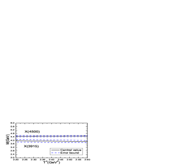
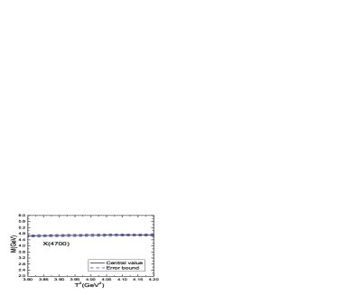
Figure 1: The masses with variations of the Borel parameters $T^{2}$.

Then we take the central values of the predicted masses and pole residues as the input parameters, and obtain the corresponding pole contributions of the $X(3915)$ and $X(4500)$ respectively,

$${\rm pole}_{X(3915)} = (56-77)\%\,,$$

$${\rm pole}_{X(4500)} = (14-18)\%\,,$$ (44)

at the energy scale $\mu=1.45\,\rm{GeV}$ and

$${\rm pole}_{X(3915)} = (44-65)\%\,,$$

$${\rm pole}_{X(4500)} = (30-38)\%\,,$$ (45)

at the energy scale $\mu=2.65\,\rm{GeV}$.

It is more reliable to extract the masses and pole residues from the QCD sum rules with larger pole contributions. The pole contribution of the $X(3915)$ at $\mu=1.45\,\rm{GeV}$ is larger than that at $\mu=2.65\,\rm{GeV}$, we prefer to extract the mass and pole residue of the $X(3915)$ at $\mu=1.45\,\rm{GeV}$ and discard the ones at $\mu=2.65\,\rm{GeV}$. On the other hand, the pole contribution of the $X(4500)$ at $\mu=2.65\,\rm{GeV}$ is larger than that at $\mu=1.45\,\rm{GeV}$, we prefer to extract the mass and pole residue of the $X(4500)$ at $\mu=2.65\,\rm{GeV}$ and discard the ones at $\mu=1.45\,\rm{GeV}$. In this article, we take the referred values

$$M_{X(3915)} = 3.92^{+0.19}_{-0.18}\,\rm{GeV}\,,\,\,\,{\rm Experimental\,\,value}\,\,\,\,3918.4\pm 1.9\,\rm{MeV}\,\cite[cite]{[\@@bibref{}{PDG}{}{}]}\,,$$

$$M_{X(4500)} = 4.50^{+0.08}_{-0.09}\,\rm{GeV}\,,\,\,\,{\rm Experimental\,\,value}\,\,\,\,4506\pm 11^{+12}_{-15}\rm{MeV}\,\cite[cite]{[\@@bibref{}{LHCb2016}{}{}]}\,,$$

$$\lambda_{X(3915)} = 3.90^{+1.73}_{-1.12}\times 10^{-2}\,\rm{GeV}^{5}\,,$$

$$\lambda_{X(4500)} = 1.21^{+0.18}_{-0.14}\times 10^{-1}\,\rm{GeV}^{5}\,,$$ (46)

as the physical values. The predicted masses $M_{X(3915)}=3.92^{+0.19}_{-0.18}\,\rm{GeV}$, $M_{X(4500)}=4.50^{+0.08}_{-0.09}\,\rm{GeV}$, $M_{X(4700)}=4.70^{+0.08}_{-0.09}\,\rm{GeV}$ satisfy the energy scale formula in Eq.(30).

The predicted masses $M_{X(3915)}=3.92^{+0.19}_{-0.18}\,\rm{GeV}$, $M_{X(4500)}=4.50^{+0.08}_{-0.09}\,\rm{GeV}$, $M_{X(4700)}=4.70^{+0.08}_{-0.09}\,\rm{GeV}$, which are shown explicitly in Fig.1, are in excellent agreement with the experimental data, the present calculations support assigning the $X(3915)$ and $X(4500)$ to be the ground state and the first radial excited state of the $C\gamma_{\mu}\otimes\gamma^{\mu}C$ type $cs\bar{c}\bar{s}$ tetraquark states, and assigning the $X(4700)$ to be the ground state $C\gamma_{\mu}\gamma_{5}\otimes\gamma_{5}\gamma^{\mu}C$ type $cs\bar{c}\bar{s}$ tetraquark state.

Now we study the finite width effects on the predicted tetraquark masses. The currents $J(x)$ and $J_{5}(x)$ couple potentially with the scattering states $J/\psi\phi$, $D_{s}\bar{D}_{s}$, $D_{s}^{*}\bar{D}^{*}_{s}$, $\cdots$, we take into account the contributions of the intermediate meson-loops to the correlation functions $\Pi(p^{2})$ and $\Pi_{5}(p^{2})$,

$$\Pi(p^{2}) = -\frac{\widehat{\lambda}_{X(3915)}^{2}}{p^{2}-\widehat{M}_{X(3915)}^{2}-\Sigma^{X(3915)}_{J/\psi\phi}(p)+\cdots}-\frac{\widehat{\lambda}_{X(4500)}^{2}}{p^{2}-\widehat{M}_{X(4500)}^{2}-\Sigma^{X(4500)}_{J/\psi\phi}(p)+\cdots}+\cdots\,,$$

$$\Pi_{5}(p^{2}) = -\frac{\widehat{\lambda}_{X(4700)}^{2}}{p^{2}-\widehat{M}_{X(4700)}^{2}-\Sigma^{X(4700)}_{J/\psi\phi}(p)+\cdots}+\cdots\,,$$ (47)

where the $\widehat{\lambda}_{X(3915/4500/4700)}$ and $\widehat{M}_{X(3915/4500/4700)}$ are bare quantities to absorb the divergences in the self-energies $\Sigma^{X(3915/4500/4700)}_{J/\psi\phi}(p)$, $\cdots$. All the renormalized self-energies contribute a finite imaginary part to modify the dispersion relation,

$$\Pi(p^{2}) = -\frac{\lambda_{X(3915)}^{2}}{p^{2}-M_{X(3915)}^{2}+i\sqrt{p^{2}}\Gamma_{X(3915)}(p^{2})}-\frac{\lambda_{X(4500)}^{2}}{p^{2}-M_{X(4500)}^{2}+i\sqrt{p^{2}}\Gamma_{X(4500)}(p^{2})}+\cdots\,,$$

$$\Pi_{5}(p^{2}) = -\frac{\lambda_{X(4700)}^{2}}{p^{2}-M_{X(4700)}^{2}+i\sqrt{p^{2}}\Gamma_{X(4700)}(p^{2})}+\cdots\,.$$ (48)

We take into account the finite width effects by the following simple replacements of the hadronic spectral densities,

$$\delta\left(s-M^{2}_{X(3915/4500/4700)}\right) \to \frac{1}{\pi}\frac{\sqrt{s}\,\Gamma_{X(3915/4500/4700)}(s)}{\left(s-M_{X(3915/4500/4700)}^{2}\right)^{2}+s\,\Gamma_{X(3915/4500/4700)}^{2}(s)}\,,$$ (49)

where

$$\Gamma_{X(3915/4500/4700)}(s) = \Gamma_{X(3915/4500/4700)}\frac{M^{2}_{X(3915/4500/4700)}}{s}\,.$$ (50)

The experimental values of the widths are $\Gamma_{X(3915)}=20\pm 5\,\rm{MeV}$ [9], $\Gamma_{X(4500)}=92\pm 21^{+21}_{-20}\,\rm{MeV}$, $\Gamma_{X(4700)}=120\pm 31^{+42}_{-33}\,\rm{MeV}$ [5].

Then the phenomenological sides of the QCD sum rules in Eqs.(18-19) undergo the following changes,

$$B_{T}^{2}\Pi = \lambda^{2}_{X(3915)}\exp\left(-\frac{M^{2}_{X(3915)}}{T^{2}}\right)+\lambda^{2}_{X(4500)}\exp\left(-\frac{M^{2}_{X(4500)}}{T^{2}}\right)$$ (51)

$$\to \frac{\lambda^{2}_{X(3915)}}{\pi}\int_{(M_{J/\psi}+M_{\omega})^{2}}^{s^{0}_{X(4500)}}ds\frac{\sqrt{s}\,\Gamma_{X(3915)}(s)}{(s-M_{X(3915)}^{2})^{2}+s\Gamma_{X(3915)}^{2}(s)}\exp\left(-\frac{s}{T^{2}}\right)$$

$$+\frac{\lambda^{2}_{X(4500)}}{\pi}\int_{(M_{J/\psi}+M_{\phi})^{2}}^{s^{0}_{X(4500)}}ds\frac{\sqrt{s}\,\Gamma_{X(4500)}(s)}{(s-M_{X(4500)}^{2})^{2}+s\Gamma_{X(4500)}^{2}(s)}\exp\left(-\frac{s}{T^{2}}\right)$$

$$= 0.97\,\left\{\lambda^{2}_{X(3915)}\exp\left(-\frac{M^{2}_{X(3915)}}{T^{2}}\right)+\lambda^{2}_{X(4500)}\exp\left(-\frac{M^{2}_{X(4500)}}{T^{2}}\right)\right\}\,,$$

$$B_{T}^{2}\Pi_{5} = \lambda^{2}_{X(4700)}\exp\left(-\frac{M^{2}_{X(4700)}}{T^{2}}\right)$$ (52)

$$\to \frac{\lambda^{2}_{X(4700)}}{\pi}\int_{(M_{J/\psi}+M_{\phi})^{2}}^{s^{0}_{X(4700)}}ds\frac{\sqrt{s}\,\Gamma_{X(4700)}(s)}{(s-M_{X(4700)}^{2})^{2}+s\Gamma_{X(4700)}^{2}(s)}\exp\left(-\frac{s}{T^{2}}\right)$$

$$= 0.99\,\lambda^{2}_{X(4700)}\exp\left(-\frac{M^{2}_{X(4700)}}{T^{2}}\right)\,,$$

and

$$-\frac{1}{d(1/T^{2})}B_{T}^{2}\Pi = M^{2}_{X(3915)}\lambda^{2}_{X(3915)}\exp\left(-\frac{M^{2}_{X(3915)}}{T^{2}}\right)+M^{2}_{X(4500)}\lambda^{2}_{X(4500)}\exp\left(-\frac{M^{2}_{X(4500)}}{T^{2}}\right)$$ (53)

$$\to \frac{\lambda^{2}_{X(3915)}}{\pi}\int_{(M_{J/\psi}+M_{\omega})^{2}}^{s^{0}_{X(4500)}}ds\,s\,\frac{\sqrt{s}\,\Gamma_{X(3915)}(s)}{(s-M_{X(3915)}^{2})^{2}+s\Gamma_{X(3915)}^{2}(s)}\exp\left(-\frac{s}{T^{2}}\right)$$

$$+\frac{\lambda^{2}_{X(4500)}}{\pi}\int_{(M_{J/\psi}+M_{\phi})^{2}}^{s^{0}_{X(4500)}}ds\,s\,\frac{\sqrt{s}\,\Gamma_{X(4500)}(s)}{(s-M_{X(4500)}^{2})^{2}+s\Gamma_{X(4500)}^{2}(s)}\exp\left(-\frac{s}{T^{2}}\right)$$

$$= 0.97\,\left\{M^{2}_{X(3915)}\lambda^{2}_{X(3915)}\exp\left(-\frac{M^{2}_{X(3915)}}{T^{2}}\right)\right.$$

$$\left.+M^{2}_{X(4500)}\lambda^{2}_{X(4500)}\exp\left(-\frac{M^{2}_{X(4500)}}{T^{2}}\right)\right\}\,,$$

$$-\frac{1}{d(1/T^{2})}B_{T}^{2}\Pi_{5} = M^{2}_{X(4700)}\lambda^{2}_{X(4700)}\exp\left(-\frac{M^{2}_{X(4700)}}{T^{2}}\right)$$ (54)

$$\to \frac{\lambda^{2}_{X(4700)}}{\pi}\int_{(M_{J/\psi}+M_{\phi})^{2}}^{s^{0}_{X(4700)}}ds\,s\,\frac{\sqrt{s}\,\Gamma_{X(4700)}(s)}{(s-M_{X(4700)}^{2})^{2}+s\Gamma_{X(4700)}^{2}(s)}\exp\left(-\frac{s}{T^{2}}\right)$$

$$= 0.99\,M^{2}_{X(4700)}\lambda^{2}_{X(4700)}\exp\left(-\frac{M^{2}_{X(4700)}}{T^{2}}\right)\,,$$

where the $B_{T^{2}}$ denotes the Borel transformation. So we can absorb the numerical factors $0.97$ and $0.99$ into the pole residues $\lambda_{X(3915/4500)}$ and $\lambda_{X(4700)}$ safely, the intermediate meson-loops cannot affect the predicted masses $M_{X(3915/4500/4700)}$ significantly, the zero width approximation in the phenomenological spectral densities works.

4 Conclusion

In this article, we tentatively assign the $X(3915)$ and $X(4500)$ to be ground state and the first radial excited state of the $C\gamma_{\mu}\otimes\gamma^{\mu}C$ type $cs\bar{c}\bar{s}$ tetraquark states, respectively, assign the $X(4700)$ to be the ground state $C\gamma_{\mu}\gamma_{5}\otimes\gamma_{5}\gamma^{\mu}C$ type $cs\bar{c}\bar{s}$ tetraquark state, construct the corresponding interpolating currents, and study their masses and pole residues with the QCD sum rules by calculating the contributions of the vacuum condensates up to dimension 10 in the operator product expansion. Moreover, we use the energy scale formula $\mu=\sqrt{M^{2}_{X/Y/Z}-(2{\mathbb{M}}_{c})^{2}}$ to determine the ideal energy scales of the QCD spectral densities. The numerical results support assigning the $X(3915)$ and $X(4500)$ to be the ground state and the first radial excited state of the $C\gamma_{\mu}\otimes\gamma^{\mu}C$ type $cs\bar{c}\bar{s}$ tetraquark states, respectively, and assigning the $X(4700)$ to be the ground state of the $C\gamma_{\mu}\gamma_{5}\otimes\gamma_{5}\gamma^{\mu}C$ type $cs\bar{c}\bar{s}$ tetraquark state.

Appendix

The explicit expression of the QCD spectral density $\rho(s)$,

$$\rho(s) = \frac{1}{256\pi^{6}}\int_{y_{i}}^{y_{f}}dy\int_{z_{i}}^{1-y}dz\,yz\,(1-y-z)^{3}\left(s-\overline{m}_{c}^{2}\right)^{2}\left(7s^{2}-6s\overline{m}_{c}^{2}+\overline{m}_{c}^{4}\right)$$

$$+\frac{1}{256\pi^{6}}\int_{y_{i}}^{y_{f}}dy\int_{z_{i}}^{1-y}dz\,yz\,(1-y-z)^{2}\left(s-\overline{m}_{c}^{2}\right)^{3}\left(3s-\overline{m}_{c}^{2}\right)$$

$$+\frac{m_{s}m_{c}}{128\pi^{6}}\int_{y_{i}}^{y_{f}}dy\int_{z_{i}}^{1-y}dz\,(y+z)\,(1-y-z)^{2}\left(s-\overline{m}_{c}^{2}\right)^{2}\left(5s-2\overline{m}_{c}^{2}\right)$$

$$-\frac{m_{c}\langle\bar{s}s\rangle}{8\pi^{4}}\int_{y_{i}}^{y_{f}}dy\int_{z_{i}}^{1-y}dz\,(y+z)(1-y-z)\left(s-\overline{m}_{c}^{2}\right)\left(2s-\overline{m}_{c}^{2}\right)$$

$$+\frac{m_{s}\langle\bar{s}s\rangle}{8\pi^{4}}\int_{y_{i}}^{y_{f}}dy\int_{z_{i}}^{1-y}dz\,yz(1-y-z)\left(10s^{2}-12s\overline{m}_{c}^{2}+3\overline{m}_{c}^{4}\right)$$

$$+\frac{m_{s}\langle\bar{s}s\rangle}{8\pi^{4}}\int_{y_{i}}^{y_{f}}dy\int_{z_{i}}^{1-y}dz\,yz\left(s-\overline{m}_{c}^{2}\right)\left(2s-\overline{m}_{c}^{2}\right)$$

$$-\frac{m_{s}m_{c}^{2}\langle\bar{s}s\rangle}{2\pi^{4}}\int_{y_{i}}^{y_{f}}dy\int_{z_{i}}^{1-y}dz\left(s-\overline{m}_{c}^{2}\right)$$

$$-\frac{m_{c}^{2}}{192\pi^{4}}\langle\frac{\alpha_{s}GG}{\pi}\rangle\int_{y_{i}}^{y_{f}}dy\int_{z_{i}}^{1-y}dz\left(\frac{z}{y^{2}}+\frac{y}{z^{2}}\right)(1-y-z)^{3}$$

$$\left\{2s-\overline{m}_{c}^{2}+\frac{\overline{m}_{c}^{4}}{6}\delta\left(s-\overline{m}_{c}^{2}\right)\right\}$$

$$-\frac{m_{c}^{2}}{384\pi^{4}}\langle\frac{\alpha_{s}GG}{\pi}\rangle\int_{y_{i}}^{y_{f}}dy\int_{z_{i}}^{1-y}dz\left(\frac{z}{y^{2}}+\frac{y}{z^{2}}\right)(1-y-z)^{2}\left(3s-2\overline{m}_{c}^{2}\right)$$

$$-\frac{1}{768\pi^{4}}\langle\frac{\alpha_{s}GG}{\pi}\rangle\int_{y_{i}}^{y_{f}}dy\int_{z_{i}}^{1-y}dz\left(y+z\right)(1-y-z)^{2}\left(10s^{2}-12s\overline{m}_{c}^{2}+3\overline{m}_{c}^{4}\right)$$

$$+\frac{1}{384\pi^{4}}\langle\frac{\alpha_{s}GG}{\pi}\rangle\int_{y_{i}}^{y_{f}}dy\int_{z_{i}}^{1-y}dz\left(y+z\right)(1-y-z)\left(s-\overline{m}_{c}^{2}\right)\left(2s-\overline{m}_{c}^{2}\right)$$

$$+\frac{1}{384\pi^{4}}\langle\frac{\alpha_{s}GG}{\pi}\rangle\int_{y_{i}}^{y_{f}}dy\int_{z_{i}}^{1-y}dz\left(y+z\right)(1-y-z)^{2}\left(10s^{2}-12s\overline{m}_{c}^{2}+3\overline{m}_{c}^{4}\right)$$

$$+\frac{1}{3456\pi^{4}}\langle\frac{\alpha_{s}GG}{\pi}\rangle\int_{y_{i}}^{y_{f}}dy\int_{z_{i}}^{1-y}dz\,(1-y-z)^{3}\left(10s^{2}-12s\overline{m}_{c}^{2}+3\overline{m}_{c}^{4}\right)$$

$$+\frac{1}{576\pi^{4}}\langle\frac{\alpha_{s}GG}{\pi}\rangle\int_{y_{i}}^{y_{f}}dy\int_{z_{i}}^{1-y}dz\,yz\,(1-y-z)\left(10s^{2}-12s\overline{m}_{c}^{2}+3\overline{m}_{c}^{4}\right)$$

$$+\frac{1}{576\pi^{4}}\langle\frac{\alpha_{s}GG}{\pi}\rangle\int_{y_{i}}^{y_{f}}dy\int_{z_{i}}^{1-y}dz\,(1-y-z)^{2}\left(s-\overline{m}_{c}^{2}\right)\left(2s-\overline{m}_{c}^{2}\right)$$

$$+\frac{1}{288\pi^{4}}\langle\frac{\alpha_{s}GG}{\pi}\rangle\int_{y_{i}}^{y_{f}}dy\int_{z_{i}}^{1-y}dz\,yz\left(s-\overline{m}_{c}^{2}\right)\left(2s-\overline{m}_{c}^{2}\right)$$

$$+\frac{m_{c}\langle\bar{s}g_{s}\sigma Gs\rangle}{32\pi^{4}}\int_{y_{i}}^{y_{f}}dy\int_{z_{i}}^{1-y}dz\,(y+z)\left(3s-2\overline{m}_{c}^{2}\right)$$

$$-\frac{m_{c}\langle\bar{s}g_{s}\sigma Gs\rangle}{48\pi^{4}}\int_{y_{i}}^{y_{f}}dy\int_{z_{i}}^{1-y}dz\,(1-y-z)\left(3s-2\overline{m}_{c}^{2}\right)$$

$$-\frac{m_{s}\langle\bar{s}g_{s}\sigma Gs\rangle}{8\pi^{4}}\int_{y_{i}}^{y_{f}}dy\int_{z_{i}}^{1-y}dz\,yz\left\{2s-\overline{m}_{c}^{2}+\frac{\overline{m}_{c}^{2}}{6}\delta\left(s-\overline{m}_{c}^{2}\right)\right\}$$

$$-\frac{m_{s}\langle\bar{s}g_{s}\sigma Gs\rangle}{48\pi^{4}}\int_{y_{i}}^{y_{f}}dy\,y(1-y)\left(3s-2\widetilde{m}_{c}^{2}\right)$$

$$+\frac{m_{s}m_{c}^{2}\langle\bar{s}g_{s}\sigma Gs\rangle}{8\pi^{4}}\int_{y_{i}}^{y_{f}}dy$$

$$-\frac{m_{s}m_{c}^{2}\langle\bar{s}g_{s}\sigma Gs\rangle}{48\pi^{4}}\int_{y_{i}}^{y_{f}}dy\int_{z_{i}}^{1-y}dz\left(\frac{1}{y}+\frac{1}{z}\right)$$

$$+\frac{m_{c}^{2}\langle\bar{s}s\rangle^{2}}{3\pi^{2}}\int_{y_{i}}^{y_{f}}dy+\frac{g_{s}^{2}\langle\bar{s}s\rangle^{2}}{54\pi^{4}}\int_{y_{i}}^{y_{f}}dy\int_{z_{i}}^{1-y}dz\,yz\left\{2s-\overline{m}_{c}^{2}+\frac{\overline{m}_{c}^{4}}{6}\delta\left(s-\overline{m}_{c}^{2}\right)\right\}$$

$$+\frac{g_{s}^{2}\langle\bar{s}s\rangle^{2}}{324\pi^{4}}\int_{y_{i}}^{y_{f}}dy\,y(1-y)\left(3s-2\widetilde{m}_{c}^{2}\right)$$

$$-\frac{g_{s}^{2}\langle\bar{s}s\rangle^{2}}{648\pi^{4}}\int_{y_{i}}^{y_{f}}dy\int_{z_{i}}^{1-y}dz\,(1-y-z)\left\{3\left(\frac{z}{y}+\frac{y}{z}\right)\left(3s-2\overline{m}_{c}^{2}\right)+\left(\frac{z}{y^{2}}+\frac{y}{z^{2}}\right)\right.$$

$$\left.m_{c}^{2}\left[2+\overline{m}_{c}^{2}\delta\left(s-\overline{m}_{c}^{2}\right)\right]+(y+z)\left[12\left(2s-\overline{m}_{c}^{2}\right)+2\overline{m}_{c}^{4}\delta\left(s-\overline{m}_{c}^{2}\right)\right]\right\}$$

$$-\frac{g_{s}^{2}\langle\bar{s}s\rangle^{2}}{1944\pi^{4}}\int_{y_{i}}^{y_{f}}dy\int_{z_{i}}^{1-y}dz\,(1-y-z)\left\{15\left(\frac{z}{y}+\frac{y}{z}\right)\left(3s-2\overline{m}_{c}^{2}\right)+7\left(\frac{z}{y^{2}}+\frac{y}{z^{2}}\right)\right.$$

$$\left.m_{c}^{2}\left[2+\overline{m}_{c}^{2}\delta\left(s-\overline{m}_{c}^{2}\right)\right]+(y+z)\left[12\left(2s-\overline{m}_{c}^{2}\right)+2\overline{m}_{c}^{4}\delta\left(s-\overline{m}_{c}^{2}\right)\right]\right\}$$

$$-\frac{m_{s}m_{c}\langle\bar{s}s\rangle^{2}}{12\pi^{2}}\int_{y_{i}}^{y_{f}}dy\left\{2+\widetilde{m}_{c}^{2}\delta(s-\widetilde{m}_{c}^{2})\right\}$$

$$+\frac{m_{c}^{3}\langle\bar{s}s\rangle}{144\pi^{2}}\langle\frac{\alpha_{s}GG}{\pi}\rangle\int_{y_{i}}^{y_{f}}dy\int_{z_{i}}^{1-y}dz\left(\frac{y}{z^{3}}+\frac{z}{y^{3}}+\frac{1}{y^{2}}+\frac{1}{z^{2}}\right)(1-y-z)$$

$$\left(1+\frac{\overline{m}_{c}^{2}}{T^{2}}\right)\delta\left(s-\overline{m}_{c}^{2}\right)$$

$$-\frac{m_{c}\langle\bar{s}s\rangle}{48\pi^{2}}\langle\frac{\alpha_{s}GG}{\pi}\rangle\int_{y_{i}}^{y_{f}}dy\int_{z_{i}}^{1-y}dz\left(\frac{y}{z^{2}}+\frac{z}{y^{2}}\right)(1-y-z)\left\{2+\overline{m}_{c}^{2}\delta\left(s-\overline{m}_{c}^{2}\right)\right\}$$

$$+\frac{m_{c}\langle\bar{s}s\rangle}{48\pi^{2}}\langle\frac{\alpha_{s}GG}{\pi}\rangle\int_{y_{i}}^{y_{f}}dy\int_{z_{i}}^{1-y}dz\left\{2+\overline{m}_{c}^{2}\delta\left(s-\overline{m}_{c}^{2}\right)\right\}$$

$$-\frac{m_{c}\langle\bar{s}s\rangle}{144\pi^{2}}\langle\frac{\alpha_{s}GG}{\pi}\rangle\int_{y_{i}}^{y_{f}}dy\int_{z_{i}}^{1-y}dz\left(\frac{1-y}{y}+\frac{1-z}{z}\right)\left\{2+\overline{m}_{c}^{2}\delta\left(s-\overline{m}_{c}^{2}\right)\right\}$$

$$-\frac{m_{c}\langle\bar{s}s\rangle}{288\pi^{2}}\langle\frac{\alpha_{s}GG}{\pi}\rangle\int_{y_{i}}^{y_{f}}dy\left\{2+\widetilde{m}_{c}^{2}\,\delta\left(s-\widetilde{m}_{c}^{2}\right)\right\}$$

$$-\frac{m_{c}^{2}\langle\bar{s}s\rangle\langle\bar{s}g_{s}\sigma Gs\rangle}{6\pi^{2}}\int_{0}^{1}dy\left(1+\frac{\widetilde{m}_{c}^{2}}{T^{2}}\right)\delta\left(s-\widetilde{m}_{c}^{2}\right)$$

$$+\frac{m_{c}^{2}\langle\bar{s}s\rangle\langle\bar{s}g_{s}\sigma Gs\rangle}{36\pi^{2}}\int_{0}^{1}dy\frac{1}{y(1-y)}\delta\left(s-\widetilde{m}_{c}^{2}\right)$$

$$+\frac{m_{c}^{2}\langle\bar{s}g_{s}\sigma Gs\rangle^{2}}{48\pi^{2}T^{6}}\int_{0}^{1}dy\,\widetilde{m}_{c}^{4}\,\delta\left(s-\widetilde{m}_{c}^{2}\right)$$

$$-\frac{m_{c}^{4}\langle\bar{s}s\rangle^{2}}{54T^{4}}\langle\frac{\alpha_{s}GG}{\pi}\rangle\int_{0}^{1}dy\left\{\frac{1}{y^{3}}+\frac{1}{(1-y)^{3}}\right\}\delta\left(s-\widetilde{m}_{c}^{2}\right)$$

$$+\frac{m_{c}^{2}\langle\bar{s}s\rangle^{2}}{18T^{2}}\langle\frac{\alpha_{s}GG}{\pi}\rangle\int_{0}^{1}dy\left\{\frac{1}{y^{2}}+\frac{1}{(1-y)^{2}}\right\}\delta\left(s-\widetilde{m}_{c}^{2}\right)$$

$$+\frac{m_{c}^{2}\langle\bar{s}s\rangle^{2}}{54T^{2}}\langle\frac{\alpha_{s}GG}{\pi}\rangle\int_{0}^{1}dy\frac{1}{y(1-y)}\delta\left(s-\widetilde{m}_{c}^{2}\right)$$

$$-\frac{m_{c}^{2}\langle\bar{s}g_{s}\sigma Gs\rangle^{2}}{144\pi^{2}T^{4}}\int_{0}^{1}dy\frac{1}{y(1-y)}\widetilde{m}_{c}^{2}\,\delta\left(s-\widetilde{m}_{c}^{2}\right)$$

$$+\frac{m_{c}^{2}\langle\bar{s}g_{s}\sigma Gs\rangle^{2}}{32\pi^{2}T^{2}}\int_{0}^{1}dy\frac{1}{y(1-y)}\delta\left(s-\widetilde{m}_{c}^{2}\right)$$

$$+\frac{m_{c}^{2}\langle\bar{s}s\rangle^{2}}{54T^{6}}\langle\frac{\alpha_{s}GG}{\pi}\rangle\int_{0}^{1}dy\,\widetilde{m}_{c}^{4}\,\delta\left(s-\widetilde{m}_{c}^{2}\right)\,,$$ (55)

where $y_{f}=\frac{1+\sqrt{1-4m_{c}^{2}/s}}{2}$, $y_{i}=\frac{1-\sqrt{1-4m_{c}^{2}/s}}{2}$, $z_{i}=\frac{ym_{c}^{2}}{ys-m_{c}^{2}}$, $\overline{m}_{c}^{2}=\frac{(y+z)m_{c}^{2}}{yz}$, $\widetilde{m}_{c}^{2}=\frac{m_{c}^{2}}{y(1-y)}$, $\int_{y_{i}}^{y_{f}}dy\to\int_{0}^{1}dy$, $\int_{z_{i}}^{1-y}dz\to\int_{0}^{1-y}dz$, when the $\delta$ functions $\delta\left(s-\overline{m}_{c}^{2}\right)$ and $\delta\left(s-\widetilde{m}_{c}^{2}\right)$ appear.

References

[1] T. Aaltonen et al, Phys. Rev. Lett. 102 (2009) 242002.
[2] T. Aaltonen et al, arXiv:1101.6058.
[3] S. Chatrchyan et al, Phys. Lett. B734 (2014) 261.
[4] V. M. Abazov, Phys. Rev. D89 (2014) 012004.
[5] http://meson.if.uj.edu.pl/indico/event/3/session/1/contribution/16;
R. Aaij et al, arXiv:1606.07895; R. Aaij et al, arXiv:1606.07898.
[6] K. Yi, Int. J. Mod. Phys. A28 (2013) 1330020.
[7] Z. G. Wang and T. Huang, Phys. Rev. D89 (2014) 054019.
[8] Z. G. Wang, arXiv:1607.00701.
[9] K. A. Olive et al, Chin. Phys. C38 (2014) 090001.
[10] L. Maiani, F. Piccinini, A. D. Polosa and V. Riquer, Phys. Rev. D89 (2014) 114010.
[11] M. Nielsen and F. S. Navarra, Mod. Phys. Lett. A29 (2014) 1430005.
[12] Z. G. Wang, Commun. Theor. Phys. 63 (2015) 325.
[13] S. K. Choi et al, Phys. Rev. Lett. 94 (2005) 182002.
[14] B. Aubert et al, Phys. Rev. Lett. 101 (2008) 082001.
[15] S. Uehara et al, Phys. Rev. Lett. 104 (2010) 092001.
[16] R. F. Lebed and A. D. Polosa, Phys. Rev. D93 (2016) 094024.
[17] A. De Rujula, H. Georgi and S. L. Glashow, Phys. Rev. D12 (1975) 147;
T. DeGrand, R. L. Jaffe, K. Johnson and J. E. Kiskis, Phys. Rev. D12 (1975) 2060.
[18] Z. G. Wang, Eur. Phys. J. C71 (2011) 1524;
R. T. Kleiv, T. G. Steele and A. Zhang, Phys. Rev. D87 (2013) 125018.
[19] Z. G. Wang, Commun. Theor. Phys. 59 (2013) 451.
[20] Z. G. Wang, Eur. Phys. J. C62 (2009) 375; Z. G. Wang, Phys. Rev. D79 (2009) 094027;
Z. G. Wang, Eur. Phys. J. C67 (2010) 411.
[21] Z. G. Wang, Mod. Phys. Lett. A29 (2014) 1450207.
[22] Z. G. Wang, Commun. Theor. Phys. 63 (2015) 466;
Z. G. Wang and Y. F. Tian, Int. J. Mod. Phys. A30 (2015) 1550004.
[23] H. X. Chen, E. L. Cui, W. Chen, X. Liu and S. L. Zhu, arXiv:1606.03179.
[24] M. A. Shifman, A. I. Vainshtein and V. I. Zakharov, Nucl. Phys. B147 (1979) 385.
[25] L. J. Reinders, H. Rubinstein and S. Yazaki, Phys. Rept. 127 (1985) 1.
[26] V. A. Novikov, L. B. Okun, M. A. Shifman, A. I. Vainshtein, M. B. Voloshin and V. I. Zakharov, Phys. Rept. 41 (1978) 1.
[27] Z. G. Wang, Eur. Phys. J. C76 (2016) 427.
[28] M. S. Maior de Sousa and R. Rodrigues da Silva, arXiv:1205.6793.
[29] Z. G. Wang, Eur. Phys. J. C74 (2014) 2874.
[30] Z. G. Wang and T. Huang, Nucl. Phys. A930 (2014) 63.
[31] Z. G. Wang, Eur. Phys. J. C76 (2016) 387.
[32] P. Colangelo and A. Khodjamirian, hep-ph/0010175.