Explicit BCJ numerators of nonlinear sigma model

Abstract

In this paper, we investigate the color-kinematics duality in nonlinear sigma model (NLSM). We present explicit polynomial expressions for the kinematic numerators (BCJ numerators). The calculation is done separately in two parametrization schemes of the theory using Kawai-Lewellen-Tye relation inspired technique, both lead to polynomial numerators. We summarize the calculation in each case into a set of rules that generates BCJ numerators for all multilplicities. In Cayley parametrization we find the numerator is described by a particularly simple formula solely in terms of momentum kernel.

1 Introduction

The Color-Kinematics duality proposed by Bern, Carrasco and Johansson (BCJ) in Bern:2008qj suggests that the color factors and momentum dependent numerators of Yang-Mills amplitudes, originally prescribed through Feynman rules, can be reformulated using a set of graphical organization principles that treats them on equal footing. The BCJ numerators associated with each trivalent graph satisfies anti-symmetry and Jacobi identities that mirrors the algebraic behavior of its color counterpart. It has been realized that for such graphical organization to work, the amplitude has to satisfy linear relations, and the revere is also true. Given BCJ amplitude relations, one can be assured of the existence of BCJ numerators Monteiro:2011pc . These amplitude relations have been proven both from field theory Feng:2010my ; Cachazo:2012uq and string perspectives Stieberger:2009hq ; BjerrumBohr:2009rd . The BCJ duality has a further independent, and yet perhaps even more striking implication on gravity. When the color dependence of a Yang-Mills amplitude is swapped in exchange for another copy of kinematic numerator, the resulting double-copy formula reproduces gravity amplitude Bern:2008qj ; Bern:2010ue . At tree level this prediction has been proven using multiple (Britto-Cachazo-Feng-Witten) BCFW shifting Bern:2010yg , and is understood to be equivalent to the famous (Kawai-Lewellen-Tye) KLT relation KLT ; Kiermaier . At the moment of writing the loop level correspondence remains a conjecture, however it has been verified through accumlating evidence Bern:2010ue ; Bern:2012uf ; Bern:2013qca ; Bern:2014sna ; Mafra:2014oia ; Mafra:2014gja ; Mafra:2015mja ; Boels:2013bi ; Carrasco:2011mn ; Bjerrum-Bohr:2013iza ; Carrasco:2012ca ; Bern:2013yya ; Nohle:2013bfa ; Ochirov:2013xba ; Chiodaroli:2013upa ; Chiodaroli:2014xia ; Yuan:2012rg ; Oxburgh:2012zr ; Saotome:2012vy . In addition, Color-Kinematics duality is also known to serve as one of the criteria for counterterms and provides a guideline for the UV behavior of gravity theory. For more details we refer the readers to the comprehensive reviews Elvang:2013cua ; Carrasco:2015iwa and the references within.

In viewing of this apparent symmetry between the color and kinematics, it is tempting to think that a simple algebraic explanation might be responsible for the behavior of BCJ numerators, similar to that of its color counterpart. And indeed, a partial understanding has been achieved by studying the self-dual sector, where the cubic vertex is identified as the structure constant of area-preserving diffeomorphism algebra BjerrumBohr:2012mg ; Monteiro:2011pc . This explains at tree level the all-except-one plus helicity in $D>4$ dimensions and the ( maximally-helicity-violating) MHV amplitudes to all multiplicities. Beyond MHV, not very much is understood about the origin of its algebraic behavior, partly because determining BCJ numerators can be techinically challenging. The complexity involves in the perturbative calculation grows factorially as mutiplicity increses. In addition the numerators are known to be non-unique. The presumably existing algebraic structure can be easily obscured by generalized gauge degrees of freedom.

As it happens, Color-Kinematics duality is known to be respected by a number of different theories not limited to Yang-Mills Johansson:2015oia ; Bargheer:2012gv ; Huang:2012wr ; Monteiro:2014cda ; Luna:2015paa ; Johansson:2014zca ; Chiodaroli:2013upa ; Sondergaard:2009za ; Weinzierl:2014ava ; Naculich:2014naa ; Naculich:2015zha . It has already been pointed to exist also in e.g., QCD Chiodaroli:2015rdg , Spontaneously Broken Einstein-Yang-Mills supergravity Johansson:2015oia . The focus of this paper is on the nonlinear sigma model (NLSM), described by the chiral Lagrangian originally designed to capture the phenomenological behavior of the Golstone bosons corresponding to the $G\times G\rightarrow G$ isospin symmetry breaking. In this model the flavor group $SU(N_{f})$ plays a similar role to the color in strong interactions and can be used to define partial amplitudes and flavor ordered Feynman rules Kampf:2013vha . (For this reason we shall be using the terms color and flavor interchangeably in this paper.) It was shown earlier that amplitudes of the nonlinear sigma model (NLSM) satisfy BCJ relation which has an off-shell extension in Cayley parametrization Chen:2013fya ; Chen:2014dfa . This relation actually implies the color-kinematic duality, as in Yang-Mills theory.

We feel that the NLSM serves as an interesting practical setting to hopefully a better understanding of the kinematic algebra, in the sense that unlike the bi-adjoint scalar theory, the algebraic property is not a built-in feature of the theory, and yet the theory is known to satisfy Color-Kinematics duality, therefore leaving a puzzle as to identifying the responsible algebra, or whether there is one existing, which is similar to the puzzle posed by Yang-Mills theory. It is also not by construction a cubic theory and can perhaps therefore provide us an example as to how to systematically cope with contact terms. In addition, the duality is known to be respected by the NLSM in arbitrary dimensions, which is still another feature shared with Yang-Mills amplitudes. The NLSM numerator however, stands a good chance to be formally simpler than those of Yang-Mills because it is given by a scalar field theory and the corresponding Feynman rules completely devoid of polariztion vectors, so that they can only be composed of Mandelstam variables.

In this paper we use the KLT inspired prescription to calculate NLSM numerators Kiermaier . We choose to work in the setting when one particular leg is taken off-shell, allowing the propagator matrix to be inverted so that the numerators can be reversely determined in terms of amplitudes. The BCJ relations observed in Chen:2013fya formulated in Cayley parametrization scheme are repeatedly used to cancel poles, much like the procedure introduced in Du:2011js to prove the color-dressed KLT relations, until an explicit expression is obtained. The resulting numerator is completely pole-free and is expressible as a sum of momentum kernel

$$n_{1|2,3,\dots,n-1|n}=\sum\limits_{\sigma}{\cal S}[n-1\dots 2\mid\sigma]$$ (1.1)

over a subset of permutations explained in section 3.3. In Cayley parametrization the numerators derived from this procedure will pick up a special set of basis numerators because of the asymmetric analytic continuation. As we will explain more at the beginning of section 4 a generic numerator in this picture is by construction defined through basis numerators, which in turn are built from amplitudes. The numerators themselves do not have to possess symmetry with respect to permuting external lines. As an alternative, we present the NLSM numerator in a more symmetrical setting. We obtain BCJ relations following similar derivations to Chen:2013fya and compute the permutation symmetric numerators up to $8$ points.

This paper is organized as follows. In section 2 we briefly review the BCJ relations between NLSM amplitudes in Cayley parametrization and the KLT inspired prescription for BCJ numerators. In section 3.2, we present and prove general rules for constructing numerators in Cayley parametrization. Section 3.3 provides a graphical summary for these rules. Permutation symmetric numerators are presented in section 4. We conclude this paper in section 5. Eight-point permutation symmetric numerators are presented in the appendix.

2 Preliminaries: Color-kinematic duality and amplitude relations in NLSM

In this section we briefly review color-kinematics duality and amplitude relations in nonlinear sigma model necessary for the discussions in this paper.

2.1 KLT relation, color-kinematics duality and dual color decomposition

Ever since the discovery of the squaring identities between gravity and Yang-Mills amplitudes of Kawai, Lewellen and Tye (KLT) KLT , it has been proven that the relation applies to a number of different theories as well, by taking the field theory limit of various closed and open string amplitudes (see, e.g. Bern:2002kj and the references therein). For example it was realized that the full Yang-Mills amplitude $M(1,2,\dots,n)$ factorizes into products of a color-dressed scalar amplitude $\widetilde{A}(n,\sigma_{2,n-1},1)$ and a color-ordered Yang-Mills amplitude $A(1,\rho_{2,n-1},n)$ Bern:1999bx . These relations are known to be expressible in manifestly $(n-2)!$ permutation symmetric form

$${M}(1,2,\dots,n)=(-1)^{n}\sum\limits_{\sigma,\rho}\widetilde{A}(n,\sigma_{2,n-1},1){{\cal S}[\sigma_{2,n-1}\mid\rho_{2,n-1}]\over k_{n}^{2}}A(1,\rho_{2,n-1},n)$$ (2.1)

and the $(n-3)!$ symmetric form

$$M(1,2,\dots,n)=(-1)^{n+1}\sum\limits_{\sigma,\rho}\widetilde{A}(n-1,n,\sigma_{2,n-1},1){\cal S}[\sigma_{2,n-2}|\rho_{2,n-2}]A(1,\rho_{2,n-2},n-1,n),$$ (2.2)

where $\sigma_{2,\dots,j}$ denotes permutations of $2,3,\dots,j$, and the momentum kernel is defined by

$${\cal S}[i_{1},\dots,i_{k}|j_{1},\dots,j_{k}]=\prod\limits_{t=1}^{k}\left(s_{i_{t}1}+\sum\limits_{q>t}^{k}\theta(i_{t},i_{q})s_{i_{t}i_{q}}\right).$$ (2.3)

Both eq. (2.1) and eq. (2.2) treat the color scalar and the color-ordered Yang-Mills amplitudes equally. Such symmetry has been made completely manifest by the color-kinematics duality statement of Bern Carrasco and Johannson Bern:2008qj , which suggests a bi-cubic formulation of the full Yang-Mills amplitude

$${M}(1,2,\dots,n)=\sum_{\text{cubic diags }i}\frac{c_{i}n_{i}}{\prod_{\alpha_{i}}s_{\alpha_{i}}}.$$ (2.4)

The kinematic numerators $n_{i}$ are assumed to satisfy the same algebraic identities as their color counterparts $c_{i}$

$${\rm antisymmetry}: c_{i}\rightarrow-c_{i}\Rightarrow n_{i}\rightarrow-n_{i}$$

$${\rm Jacobi-like~{}identity}: c_{i}+c_{j}+c_{k}=0\Rightarrow n_{i}+n_{j}+n_{k}=0.~{}~{}$$ (2.5)

Furthermore, it was realized that when the color factors $c_{i}$ are replaced by another copy of the BCJ numerators, equation (2.4) reproduces gravity Bern:2008qj ; Bern:2010ue . In viewing of the fact that the same algebraic properties are shared between color and kinematic structures, it is natural to expect that various BCJ-dual color decompositions also describe Yang-Mills amplitude. In particular it can be decomposed using half ladder kinematic factors $n_{1|\sigma(2,..,n-1)|n}$,

$$M(1,2,\dots,n)=\sum_{\sigma}n_{1|\sigma_{2,n-2}|n}\widetilde{A}(1,\sigma_{2,n-2},n),$$ (2.6)

similarly to the decomposition illustrated in DelDuca:1999rs , which we shall refer to as the dual Del Duca-Dixon-Maltoni (DDM) form in this paper.

2.1.1 The construction of BCJ numertators from KLT relation

In practice, solving the BCJ numerators can be a challenging task even if the BCJ duality in a theory has been verified. Considering the fact that amplitudes depends on numerators only linearly, in principle one can determine the numerators from amplitudes by inverting the propagator matrix. However a subtlety arises because of the singular nature of the propagator matrix. It is known that the inverse is not unique and one has to choose a specific generalized gauge Boels:2012sy . Notably one formally simple set of solutions was found using the KLT orthogonality Cachazo:2013iea . And indeed, as a matter of fact it was realized earlier that one can readily arrive at a prescription of the numerators in terms of momentum kernel by comparing the (n-3)! symmetric form of the KLT relation (2.2) with the dual color decomposition formula (2.6) Kiermaier ; BjerrumBohr:2010hn ; Naculich:2014rta ; Fu:2014pya .

Given the above set of solutions, because of the generalized gauge degrees of freedom, identifying the algebraic structure can still be quite non-trivial. Generically the half ladder numerators obtained through the algorithm just described may not simply correspond to a string of structure constants, but to a gauge transformed, linear combination of several strings of structure constants. An alternative solution to this dilemma is to tentatively make the propagator matrix non-singular through analytic continuation, and take the on-shell limit afterwards. In the language of KLT this corresponds to comparing the $(n-2)!$ symmetric form (2.1) with the dual color decomposition, and write

$$n_{1|\alpha_{2,n-2}|n}=\sum\limits_{\beta}{{\cal S}[\alpha_{2,n-2}^{T}|\beta_{2,n-2}]\over k_{n}^{2}}A\left(1,\beta_{2,n-2},n\right).$$ (2.7)

It has been recently proven by Mafra in Mafra:2016ltu that such prescription agrees with the Berends-Giele construction in the case of a bi-adjoint scalar theory, therefore yielding the non-gauge transformed algebraic factor as the half ladder numerator.

At first sight, equation (2.7) may not be very “good-looking” because the vanishing $k_{n}^{2}$ seems to lead to a divergence. However we will see in the following that this divergence is canceled by BCJ relations. In section 3 we will start from this $(n-2)!$ permutation symmetric form of the numerator prescription and see that the right hand side of this equation actually completely reduced to polynomials of Mandelstam variables $s_{ij}$. The resulting BCJ numerators therefore carries no pole.

2.2 Cayley parametrization and the nonlinear sigma model

In this paper we are interested in finding the BCJ numerators of the $SU(N_{f})$ nonlinear sigma model. This is the effective model describes the low energy behavior of Goldstone bosons associated with $SU(N_{f})\times SU(N_{f})\rightarrow SU(N_{f})$ symmetry breaking. The tree level amplitude of the Goldstone bosons was previously observed to possess color-kinematics duality Chen:2013fya .

2.2.1 Feynman rules and Berends-Giele currents in Cayley parameterization

The Lagrangian of the $SU(N_{f})$ non-linear sigma model is

$$\mathcal{L}={F^{2}\over 4}\mathop{\rm Tr}(\partial_{\mu}U\partial^{\mu}U^{\dagger}),$$ (2.8)

where $F$ is the decay constant. Each $U$ is defined in Caylay parametrization as

$$U=1+2\sum\limits_{n=1}^{\infty}\left({1\over 2F}\phi\right)^{n},~{}~{}~{}~{}$$ (2.9)

where $\phi=\sqrt{2}\phi^{a}t^{a}$, and $t^{a}$ are generators of the $SU(N_{f})$ flavor Lie algebra. It was demonstrated in Kampf:2012fn ; Kampf:2013vha that partial amplitudes and flavor-ordered Feynman rules can be defined by complete analogy to the color-ordering of Yang-Mills. For this reason we will abuse the terminology a bit in this paper and simply refer the $SU(N_{f})$ flavor as color. For future references we list the flavor ordered vertices as follows.

$$V_{2n+1} = 0,$$

$$V_{2n+2} = \left(-{1\over 2F^{2}}\right)^{n}\left(\sum\limits_{i=0}^{n}p_{2i+1}\right)^{2}=\left(-{1\over 2F^{2}}\right)^{n}\left(\sum\limits_{i=0}^{n}p_{2i+2}\right)^{2}.$$ (2.10)

It is known that vertices of odd multiplicities vanish in the Cayley parametrization scheme. Thus when an $n$-point amplitude of NLSM is referred, unless otherwise mentioned the $n$ is always understood as an even number. Note that the two expressions on the right hand side of equation (2.10) are equivalent when momentum conservation is taken into account.

Given the Feynman rules above, we can construct tree level off-shell currents with one off-shell line through Berends-Giele recursion

$$J(1,2,...,n-1)$$

$$= \frac{i}{P_{1,n-1}^{2}}\sum\limits_{m=4}^{n}\sum\limits_{0=j_{0}<j_{1}<\cdots<j_{m-1}=n-1}iV_{m}(P_{j_{0}+1,j_{1}},\cdots,P_{j_{m-2}+1,n-1},p_{n}=-P_{1,n-1})\times\prod\limits_{k=0}^{m-2}J(j_{k}+1,\cdots,j_{k+1}),$$

where $p_{n}=-P_{1,n-1}\equiv-(p_{1}+p_{2}+\dots+p_{n-1})$. The starting point of this recursion is $J(1)=J(2)=\dots=J(n-1)=1$. Note that building up an odd multiplicity current (including the off-shell line) requires at least one odd multiplicity vertex, therefore $J(2,\dots,2m+1)=0$. Even multiplicity currents in general are bulit up only by odd numbers of even sub-currents (i. e., those sub-currents with an odd number of on-shell lines and one off-shell line).

2.2.2 Amplitude relations in NLSM

It was pointed out in Chen:2013fya that off-shell currents in Cayley parametrization satisfy an off-shell version of the $U(1)$ decoupling identity and the fundamental BCJ relation, both of these two relations are restored to their more familiar original forms in the on-shell limit. Furthermore, it was noted that the $(n-2)!$ symmetric formula of KLT relation is also restored on-shell. Explicit formulas of these relations are given as follows.

• $U(1)$ identity in NLSM

  The $U(1)$ identity for off-shell currents is given by

  $$\sum\limits_{\sigma\in OP(\{\alpha_{1}\}\bigcup\{\beta_{1},\dots,\beta_{2m}\})}J(\{\sigma\})={1\over 2F^{2}}\sum\limits_{divisions\{\beta\}\rightarrow\{B_{1}\},\{B_{2}\}}J(\{B_{1}\})J(\{B_{2}\}),$$ (2.12)

  where, on the left hand side, we sum over all the possible permutations with the relative order in set $\{\beta\}$ and the relative order in set $\{\alpha\}$ kept fixed. In this paper we only need to consider when there is only one element $\alpha_{1}$ in $\{\alpha\}$ (the $U(1)$ decoupling identity) although generically the number of elements in $\{\alpha\}$ and $\{\beta\}$ can be quite arbitrary. On the right hand side, we divide the ordered set $\{\beta_{1},\dots,\beta_{2m}\}$ into two nonempty ordered subsets, each containing an odd number of elements. For example, suppose if we have six $\beta$’s in the original set $\{\beta\}$, the following three different distributions of $\beta$’s into $\{B_{1}\}$ and $\{B_{2}\}$ should be included in the summation: $\{B_{1}\}=\{\beta_{1}\}$, $\{B_{2}\}=\{\beta_{2},\dots,\beta_{6}\}$; $\{B_{1}\}=\{\beta_{1},\beta_{2},\beta_{3}\}$, $\{B_{2}\}=\{\beta_{4},\beta_{5},\beta_{6}\}$ and $\{B_{1}\}=\{\beta_{1},\dots,\beta_{5}\}$, $\{B_{2}\}=\{\beta_{6}\}$.

• Fundamental BCJ relation in NLSM

  The fundamental BCJ relation is expressible as

  $$\sum\limits_{\sigma\in OP(\{\alpha_{1}\}\bigcup\{\beta_{1},\dots,\beta_{2m-1}\})}\left(\sum\limits_{\xi_{\sigma_{i}}<\xi_{\alpha_{1}}}s_{\alpha_{1}\sigma_{i}}+s_{\alpha_{1}n}\right)J(\{\sigma\},\beta_{2m})$$ (2.13)

  $$= -{1\over 2F^{2}}\sum\limits_{divisions\{\beta\}\rightarrow\{B_{1}\},\{B_{2}\}}\left[\sum\limits_{\beta_{i}\in\{B_{2}\}}s_{\alpha_{1}\beta_{i}}J(\{B_{1}\})J(\{B_{2}\})\right],$$

  where we use $\xi_{i}$ to denote the position of the leg $i$ in permutation $\sigma$ and we always have a term $s_{\alpha_{1}n}\equiv 2p_{\alpha_{1}}\cdot p_{n}$ in the coefficients of each currents on the left hand side. On the right hand side, the summation runs over all the possible distributions of the ordered set $\{\beta\}$ into two sub-ordered sets $\{B_{1}\}$ and $\{B_{2}\}$. Since $J(\{B_{1}\})$ or $J(\{B_{2}\})$ must vanish when $\{B_{1}\}$ or $\{B_{2}\}$ is even, the surviving distributions are those with both $\{B_{1}\}$ and $\{B_{2}\}$ odd.

  When we multiply a factor $-s_{\alpha_{1}n}$ to both sides of the $U(1)$ identity eq. (2.12) and add it to the fundamental BCJ relation eq. (2.14), we get another form of the fundamental BCJ relation

  $$\sum\limits_{\sigma\in OP(\{\alpha_{1}\}\bigcup\{\beta_{2},\dots,\beta_{2m}\})}\sum\limits_{\xi_{\sigma_{i}}<\xi_{\alpha_{1}}}s_{\alpha_{1}\sigma_{i}}J(\beta_{1},\{\sigma\})$$ (2.14)

  $$= {1\over 2F^{2}}\sum\limits_{divisions\{\beta\}\rightarrow\{B_{1}\},\{B_{2}\}}\left[\sum\limits_{\beta_{i}\in\{B_{1}\}}s_{\alpha_{1}\beta_{i}}J(\{B_{1}\})J(\{B_{2}\})\right],$$

  (Assuming momentum conservation $-\left(\sum\limits_{\beta_{i}\in\{B_{2}\}}p_{\beta_{i}}+p_{n}\right)=\left(\sum\limits_{\beta_{i}\in\{B_{1}\}}p_{\beta_{i}}+p_{\alpha_{1}}\right)$ and on-shell condition $p_{\alpha_{1}}^{2}=0$ are holding.) We will be using this alternative form of the fundamental BCJ relation frequently in the following sections.

• KLT relations for color-dressed amplitudes in NLSM

  The on-shell color-dressed amplitudes of nonlinear sigma model are also known to satisfy the same KLT relation as Yang-Mills amplitudes do. Thus we have

  $$M(1,2,\dots,n)=\sum\limits_{\sigma,\rho}\widetilde{A}(n,\sigma_{2,n-2},1){{\cal S}[\sigma_{2,n-2}\mid\rho_{2,n}]\over k_{n}^{2}}A(1,\rho_{1,2},n).$$ (2.15)

  In the next section, we will start from this $(n-2)!$ formula to construct BCJ numerators.

3 The rule for BCJ numerator in NLSM with Cayley parametrization

As already stated in section 2, once we have all BCJ numerators in dual-DDM formula, we can always construct other numerators using antisymmetry and Jacobi identities. The BCJ numerator in dual DDM formula can be directly read off from the $(n-2)!$ symmetric formula of KLT relation, although this formula contains a regulator $k_{n}^{2}\to 0$ in the denominator. In this section, we present a set of systematic construction rules of the NLSM numerator using the $(n-2)!$ symmetric formula. We find that starting from extending the momentum of leg $n$ off its mass shell, we can reduce the numerator, which was originally expressed as eq. (2.7), into simpler form containing only polynomials of Mandelstam variables, with no pole or color-ordered amplitudes in the final expression. Thus the limit $k_{n}^{2}\to 0$ can be taken directly. The main idea is the following.

• We define the off-shell extension $N_{1|\sigma_{2,n-1}|n}$ of BCJ numerator $n_{1|\sigma_{2,n-1}|n}$ (see eq. (2.7)) as

  $$N_{1|\sigma_{2,n-1}|n}=\sum\limits_{\rho}{{\cal S}[\sigma_{2,n-1}^{T}\mid\rho_{2,n-1}]}J(1,\rho_{2,n-1}),$$ (3.1)

  where the $J(1,\rho_{2,n-1})$ are currents with leg $n$ taken off-shell defined recursively through Berends-Giele recursion relation (2.2.1). When leg $n$ goes on-shell, $k_{n}^{2}J(1,\rho,n)\to A(1,\rho,n)$, therefore this off-shell extension returns to the on-shell expression eq. (2.7) of $n(1,\sigma,n)$ read off from the $(n-2)!$ symmetric KLT relation.

• Applying the off-shell $U(1)$ identity and fundamental BCJ relations repeatedly, we reduce $N_{1|\sigma_{2,n-1}|n}$ into polynomials of $s_{ij}$. The final expression of $n_{1|\sigma_{2,n-1}|n}$ is then obtained by taking the on-shell limit.

3.1 Six-point example

Before giving the general rule, let us begin with a warm-up example : The numerators of tree-level six-point NLSM amplitudes. We consider the six-point numerator in dual DDM decomposition $n_{1|2345|6}$. Numerators of the form $n_{1|\sigma_{2,n-1}|6}$ can be obtained by a relabeling. Other numerators are produced by Jacobi identity and antisymmetry.

From definition eq. (3.1), the off-shell extension of $n_{1|2345|6}$ is given by

$$N_{1|2345|6} = \sum\limits_{\rho}{\cal S}[5432|\rho_{2,5}]J\left(1,\rho_{2,5}\right).$$ (3.2)

To express this $N_{1|2345|6}$ as polynomial of Mandelstam variables, we simplify the right hand side of eq. (3.2) level by level as follows.

• Step-1 We first rewrite the sum over permutations of $\{2,3,4,5\}$ as $\sum\limits_{\gamma}\sum\limits_{\alpha\in\text{OP}(5\cup\{\gamma_{2,4}\})}$, thus the off-shell extension of numerator $n_{1|2345|6}$ becomes

  $$N_{1|2345|6} = \sum\limits_{\gamma}\sum\limits_{\alpha\in\text{OP}(5\cup\{\gamma_{2,4}\})}{\cal S}[5432|\alpha]J\left(1,\{\alpha\}\right).$$ (3.3)

  From the definition of momentum kernel (2.3), we have

  $${\cal S}[5432|\gamma_{2}\dots\gamma_{i}5\gamma_{i+1}\dots\gamma_{4}]=s_{5\gamma_{j}}{\cal S}[432|\gamma],$$ (3.4)

  where $\{\gamma_{2},\gamma_{3},\gamma_{4}\}$ can be any given permutation of $2$, $3$, $4$. Then the right hand side of eq. (3.3) reads

  $$N_{1|2345|6} = \sum\limits_{\gamma\in\text{perm}\{2,3,4\}}{\cal S}[432|\gamma]\Bigl{[}s_{51}J(1,5,\gamma_{2},\gamma_{3},\gamma_{4})+(s_{51}+s_{52})J(1,\gamma_{2},5,\gamma_{3},\gamma_{4})$$

  $$+(s_{51}+s_{52}+s_{53})J(1,\gamma_{2},\gamma_{3},5,\gamma_{4})+(s_{51}+s_{52}+s_{53}+s_{54})J(1,\gamma_{2},\gamma_{3},\gamma_{4},5)\Bigr{]}.$$

  The factor in brackets is just the left hand side of the NLSM off-shell BCJ relation, thus $N_{1|2345|6}$ can be re-expressed as

  $$N_{1|2345|6} = \sum\limits_{\gamma\in\text{perm}\{2,3,4\}}(s_{51}+s_{5\gamma_{L}}){\cal S}[432|\gamma]\left[\sum\limits_{\text{Divisions}\gamma\to\gamma_{L}\gamma_{R}}J\left(1,\gamma_{L}\right)J\left(\gamma_{R}\right)\right],$$ (3.6)

  where in the brackets the summation runs over all permutations such that each of the $J\left(1,\gamma_{L}\right)$ and $J\left(\gamma_{R}\right)$ contains an odd number of on-shell legs. Specifically, for a given permutation $\{\gamma_{2},\gamma_{3},\gamma_{4}\}$, we have the following two products in the sum over divisions

  $$J(1)J(\gamma_{2},\gamma_{3},\gamma_{4}), J(1,\gamma_{2},\gamma_{3})J(\gamma_{4}).$$ (3.7)

• Step-2 After the simplification in step-1, the number of elements in the momentum kernel is reduced by one, and the six-point currents are reduced to two lower-point ones which do not contain leg $5$. In eq. (3.6), the sum over permutations $\gamma\in\text{perm}\{2,3,4\}$ can be further re-expressed as $\sum\limits_{\xi}\sum\limits_{\text{OP}\left(4\cup\xi_{2,3}\right)}$, so that the momentum dependence on leg $4$ in each momentum kernel ${\cal S}[432|\gamma]$ factorizes

  $${\cal S}\left[432|4\xi_{2}\xi_{3}\right] = s_{41}{\cal S}\left[32|\xi_{2}\xi_{3}\right],$$

  $${\cal S}\left[432|\xi_{2}4\xi_{3}\right] = \left(s_{21}+s_{4\xi_{2}}\right){\cal S}\left[32|\xi_{2}\xi_{3}\right],$$

  $${\cal S}\left[432|\xi_{2}\xi_{3}4\right] = \left(s_{41}+s_{4\xi_{2}}+s_{4\xi_{3}}\right){\cal S}\left[32|\xi_{2}\xi_{3}\right].$$ (3.8)

  Thus the two possible divisions in eq. (3.6) can further be rearranged as follows.

  • The sum of terms containing currents of the form $J(1)J(\gamma_{2},\gamma_{3},\gamma_{4})$ is given by

    $$s_{51}\sum\limits_{\xi\in\text{perm}\{23\}}{\cal S}\left[32|\xi_{2}\xi_{3}\right]J(1)\Biggl{[}s_{41}J(4,\xi_{2},\xi_{3})+\left(s_{41}+s_{4\xi_{2}}\right)J(\xi_{2},4,\xi_{3})$$

    $$~{}~{}~{}~{}~{}~{}+\left(s_{41}+s_{4\xi_{2}}+s_{4\xi_{3}}\right)J(\xi_{2},\xi_{3},4)\Biggr{]}=s_{51}\sum\limits_{\xi\in\text{perm}\{23\}}{\cal S}\left[32|\xi_{2}\xi_{3}\right]\left(s_{41}+s_{4\xi_{2}}\right).$$ (3.9)

    Applying the off-shell $U(1)$ identity (2.12) and fundamental BCJ relation (2.14) on the sum in brackets and citing the explicit expression of ${\cal S}\left[32|\xi_{2}\xi_{3}\right]$, we then write the above solely in terms of Mandelstam variables as

    $$s_{51}\left[\left(s_{41}+s_{43}\right)s_{31}s_{21}+\left(s_{41}+s_{42}\right)(s_{31}+s_{32})s_{21}\right].$$ (3.10)

  • The sum of terms containing currents of the form $J(1,\gamma_{2},\gamma_{3})J(\gamma_{4})$ is given by

    $$\sum\limits_{\xi\in\text{perm}\{2,3\}}(s_{51}+s_{54}+s_{5\xi_{2}}){\cal S}\left[32|\xi_{2}\xi_{3}\right]\Bigl{[}s_{41}J(1,4,\xi_{2})+(s_{41}+s_{4\xi_{2}})J(1,\xi_{2},4)\Bigr{]}$$ (3.11)

    $$+ (s_{51}+s_{52}+s_{53})(s_{41}+s_{42}+s_{43})\sum\limits_{\xi\in\text{perm}\{2,3\}}{\cal S}\left[32|\xi_{2}\xi_{3}\right]J(1,\xi_{2},\xi_{3}).$$

    When applying the BCJ relation on the brackets of the first line and the second sum we obtain

    $$(s_{51}+s_{54}+s_{53})s_{41}s_{31}s_{21}+(s_{51}+s_{54}+s_{52})s_{41}(s_{31}+s_{32})s_{21}$$ (3.12)

    $$+ (s_{51}+s_{52}+s_{53})(s_{41}+s_{42}+s_{43})s_{31}s_{21}.$$

• Step-3 Finally, putting eq. (3.10) and eq. (3.12) together, we get the expression for numerator

  $$N_{1|2345|6} = s_{51}\left[\left(s_{41}+s_{43}\right)s_{31}s_{21}+\left(s_{41}+s_{42}\right)(s_{31}+s_{32})s_{21}\right]$$ (3.13)

  $$+(s_{51}+s_{54}+s_{53})s_{41}s_{31}s_{21}+(s_{51}+s_{54}+s_{52})s_{41}(s_{31}+s_{32})s_{21}$$

  $$+(s_{51}+s_{52}+s_{53})(s_{41}+s_{42}+s_{43})s_{31}s_{21}.$$

  The above expression gives precisely the BCJ numerator $n_{1|2345|6}$ as $k_{n}^{2}\to 0$.

3.2 The general rule

From the six-point example we see that the numerator defined through dual DDM decomposition can be expressed as polynomial of Mandelstam variables $s_{ij}$ if the off-shell BCJ relation is applied repeatedly. The final expression contains no pole. Now let us generalize the six-point example to arbitrary higher-point cases.

The off-shell extension of general numerator $n_{1|2,\dots,n-1|n}$ in dual DDM decomposition reads

$$N_{1|2,\dots,n-1|n}=\sum\limits_{\rho}{\cal S}[n-1,n-2,\dots,2|\rho]J\left(1,\rho_{2,n-1}\right).$$ (3.14)

For convenience, let us introduce a new notation $\mathcal{N}\left(1\{\gamma_{1}\}|\{\gamma_{2}\}|\dots|\{\gamma_{P}\}\right)$ to be called a Level-${I}$ factor

$$\mathcal{N}\left(1\{\gamma_{1}\}|\{\gamma_{2}\}|\dots|\{\gamma_{P}\}\right)$$

$$\equiv \sum\limits_{\sigma_{J=1\dots I}\in\text{perm}\{\gamma_{J}\}}{\cal S}\left[(n-I)\dots 2\mid\sigma_{1}\sigma_{2}\dots\sigma_{P}\right]J\left(1,\sigma_{1}\right)J\left(\sigma_{2}\right)\dots J\left(\sigma_{I}\right),$$

where we distribute $2,3,\dots(n-I)$ into $P\leq I$ non-ordered sets $\{\gamma_{1}\}$, $\{\gamma_{2}\}$,…,$\{\gamma_{P}\}$ such that each of $\{1,\gamma_{1}\}$, …, $\{\gamma_{P}\}$ can only contain odd number of elements. There are two boundary cases

• Level-$1$ factor is nothing but the off-shell extended numerator $N_{1|2,\dots,n-1|n}$

  $$N_{1|2,\dots,n-1|n}=\mathcal{N}\left(1\{2,3,\dots,n-1\}\right).$$ (3.16)

• Level-$(n-2)$ factor is

  $${\cal N}\left(1\mid 2\right)=s_{21}J(1)J(2)=s_{21}.$$ (3.17)

To reduce the numerator into polynomial of $s_{ij}$, we should reduce the level-$1$ factor to the level-$(n-2)$ factor. This procedure can be achieved iteratively. Let us consider a given level-$I$ factor $\mathcal{N}\left(1\{\gamma_{1}\}|\dots|\{\gamma_{K}\}|\dots|\{\gamma_{I}\}\right)$, where the largest element $n-I$ is in the set $\{\gamma_{K}\}$. From definition (3.2) we have

$$\mathcal{N}\left(1\{\gamma_{1}\}|\dots|\{\gamma_{K}\}|\dots|\{\gamma_{I}\}\right)$$ (3.18)

$$= \sum\limits_{\sigma_{J|J\neq K}\in\text{perm}\{\gamma_{J}\}}\sum\limits_{\rho\in\text{perm}\left(\{\gamma_{K}\}/(n-I)\right)}\sum\limits_{j=0}^{m}\Biggl{[}{\cal S}\left[(n-I)\dots 2\mid\sigma_{1}\dots\sigma_{K-1}\rho_{1}\dots\rho_{j}(n-I)\rho_{j+1}\dots\rho_{m}\sigma_{K+1}\dots\sigma_{J}\right]$$

$$~{}~{}~{}~{}~{}~{}~{}~{}~{}~{}~{}~{}~{}~{}~{}~{}~{}~{}~{}~{}\times J\left(1,\sigma_{1}\right)\dots J\left(\rho_{1}\dots\rho_{j}(n-I)\rho_{j+1}\dots\rho_{m}\right)\dots J\left(\sigma_{I}\right)\Biggr{]},$$

where we have rewritten the sum over permutations $\sigma_{K}\in\text{perm}\{\gamma_{K}\}$ by $\sum\limits_{\rho\in\text{perm}\left(\{\gamma_{K}\}/(n-I)\right)}\sum\limits_{j=0}^{m}$. Using factorization property of momentum kernel, we re-express the momentum kernel in the above equation as

$$\left[\sum\limits_{p=1}^{K-1}s_{(n-1)\sigma_{p}}+\sum\limits_{q=1}^{j}s_{(n-1)\rho_{q}}\right]{\cal S}[(n-I-1)\dots 2\mid\sigma_{1}\dots\sigma_{K-1}\rho_{1}\dots\rho_{j}\rho_{j+1}\dots\rho_{m}\sigma_{K+1}\dots\sigma_{J}].$$ (3.19)

Thus the factor ${\cal N}\left(1\{\gamma_{1}\}|\dots|\{\gamma_{K}\}|\dots|\{\gamma_{I}\}\right)$ can be written as

$$\mathcal{N}\left(1\{\gamma_{1}\}|\dots|\{\gamma_{K}\}|\dots|\{\gamma_{I}\}\right)$$

$$= \sum\limits_{\sigma_{J|J\neq K}\in\text{perm}\{\gamma_{J}\}}J\left(1,\sigma_{1}\right)\dots J\left(\sigma_{K-1}\right)J\left(\sigma_{K+1}\right)\dots J\left(\sigma_{I}\right)$$

$$\times\sum\limits_{\rho\in\text{perm}\left(\{\gamma_{K}\}/(n-I)\right)}{\cal S}[(n-I-1)\dots 2\mid\sigma_{1}\dots\sigma_{K-1}\rho_{1}\dots\rho_{j}\rho_{j+1}\dots\rho_{m}\sigma_{K+1}\dots\sigma_{J}]$$

$$\times\left[\sum\limits_{j=0}^{m}\left(\sum\limits_{p=1}^{K-1}s_{(n-1)\sigma_{p}}+\sum\limits_{q=1}^{j}s_{(n-1)\rho_{q}}\right)J\left(\rho_{1}\dots\rho_{j}(n-I)\rho_{j+1}\dots\rho_{m}\right)\right].$$

According to the off-shell $U(1)$ identity (2.12) and the fundamental BCJ relations (2.14), we can replace the last line by

$$\sum\limits_{\text{Divisions}\rho\to\rho_{L}\rho_{R}}\left(\sum\limits_{p=1}^{K}s_{(n-1)\sigma_{p}}+s_{(n-1)\rho_{L}}\right)J(\rho_{L})J(\rho_{R}).$$ (3.21)

Therefore, the last two lines of eq. (3.2) together become

$$\sum\limits_{\rho\in\text{perm}\left(\{\gamma_{K}\}/(n-I)\right)}\sum\limits_{\text{Divisions}\rho\to\rho_{L}\rho_{R}}{\cal S}[(n-I-1)\dots 2\mid\sigma_{1}\dots\sigma_{K-1}\rho_{1}\dots\rho_{j}\rho_{j+1}\dots\rho_{m}\sigma_{K+1}\dots\sigma_{J}]$$

$$\times\left[\left(\sum\limits_{p=1}^{K-1}s_{(n-1)\sigma_{p}}+s_{(n-1)\rho_{L}}\right)J(\rho_{L})J(\rho_{R})\right].$$ (3.22)

Rearranging the two sums above, we get

$$\sum\limits_{\rho\in\text{perm}\left(\{\gamma_{K}\}/(n-I)\right)}\sum\limits_{\text{Divisions}\rho\to\rho_{L}\rho_{R}}\to\sum\limits_{\left(\{\gamma_{K}\}/(n-I)\right)\to\gamma_{L}\gamma_{R}}\sum\limits_{\rho_{L}\in\text{perm}\{\gamma_{L}\}}\sum\limits_{\rho_{R}\in\text{perm}\{\gamma_{R}\}}$$ (3.23)

and we finally rewrite the factor $\mathcal{N}\left(1\{\gamma_{1}\}|\dots|\{\gamma_{K}\}|\dots|\{\gamma_{I}\}\right)$ by the following combination of level-$(I+1)$ factors

$$\mathcal{N}\left(1\{\gamma_{1}\}|\dots|\{\gamma_{K}\}|\dots|\{\gamma_{I}\}\right)$$

$$= \sum\limits_{\left(\{\gamma_{K}\}/(n-I)\right)\to\gamma_{L}\gamma_{R}}\left(\sum\limits_{p=1}^{K}s_{(n-1)\sigma_{p}}+s_{(n-1)\gamma_{L}}\right)\mathcal{N}\left(1\{\gamma_{1}\}|\dots|\{\gamma_{L}\}|\{\gamma_{R}\}|\dots|\{\gamma_{I}\}\right).$$

In general, we start from the level-1 factor, using the iterative relation above step by step till we do not have any momentum kernel and nontrivial currents in the expression. We finally get the polynomial expression of off-shell extension $N_{1|2,\dots,n-1|n}$ of BCJ numerator $n_{1|2,\dots,n-1|n}$.

3.2.1 Revisiting the Six-point example

As a demonstration, let us try calculating again the explicit six point off-shell extenion $N_{1|2345|6}$ of the numerator $n_{123456}$ using the iterative rule eq. (3.2) we just derived.

• We start from $N_{1|2345|6}=\mathcal{N}(1\{2345\})$. After removing leg $5$, we have

  $$\mathcal{N}(1\{2345\}) = s_{51}\mathcal{N}(1|\{234\})+(s_{51}+s_{52}+s_{53})\mathcal{N}(1\{23\}|4)+(s_{51}+s_{52}+s_{54})\mathcal{N}(1\{24\}|3)$$ (3.25)

  $$+(s_{51}+s_{53}+s_{54})\mathcal{N}(1\{34\}|2).$$

• Now we remove $4$ from $\mathcal{N}(1|\{234\})$, $\mathcal{N}(1\{23\}|4)$, $\mathcal{N}(1\{24\}|3)$ and $\mathcal{N}(1\{34\}|2)$. By doing so we get

  $$\mathcal{N}(1\{2345\})$$ (3.26)

  $$= s_{51}(s_{41}+s_{42})\mathcal{N}(1|2|3)+s_{51}(s_{41}+s_{43})\mathcal{N}(1|3|2)+(s_{51}+s_{52}+s_{53})(s_{41}+s_{42}+s_{43})\mathcal{N}(1\{23\})$$

  $$+(s_{51}+s_{52}+s_{54})s_{41}\mathcal{N}(1|2|3)+(s_{51}+s_{53}+s_{54})s_{41}\mathcal{N}(1|3|2).$$

• Then removing $3$ from $(1|2|3)$, $(1|3|2)$ and $(1\{23\})$ and we arrive at

  $$\mathcal{N}(1\{2345\}) = s_{51}(s_{41}+s_{42})(s_{31}+s_{32})\mathcal{N}(1|2)+s_{51}(s_{41}+s_{43})s_{31}\mathcal{N}(1|2)$$ (3.27)

  $$+(s_{51}+s_{52}+s_{53})(s_{41}+s_{42}+s_{43})s_{31}\mathcal{N}(1|2)+(s_{51}+s_{52}+s_{54})s_{41}(s_{31}+s_{32})\mathcal{N}(1|2)$$

  $$+(s_{51}+s_{53}+s_{54})s_{41}s_{31}\mathcal{N}(1|2).$$

• Finally, removing $2$ from $(1|2)$ and we obtain the following result.

  $$N_{1|2345|6} = \mathcal{N}(1\{2345\})$$ (3.28)

  $$= s_{51}(s_{41}+s_{42})(s_{31}+s_{32})s_{12}+s_{51}(s_{41}+s_{43})s_{31}s_{12}$$

  $$+(s_{51}+s_{52}+s_{53})(s_{41}+s_{42}+s_{43})s_{31}s_{21}+(s_{51}+s_{52}+s_{54})s_{41}(s_{31}+s_{32})s_{21}$$

  $$+(s_{51}+s_{53}+s_{54})s_{41}s_{31}s_{21},$$

  which precisely agree with the six-point result (3.13) given in the previous section.

3.3 Graphical rules and explicit numerator formula in Cayley parametrization

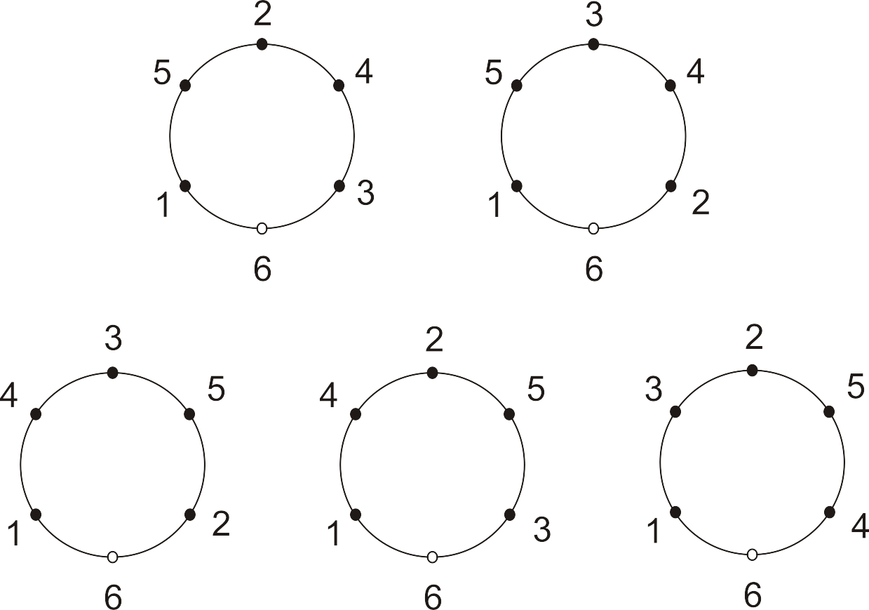
Figure 1: All possible configurations for the six-point numerator.

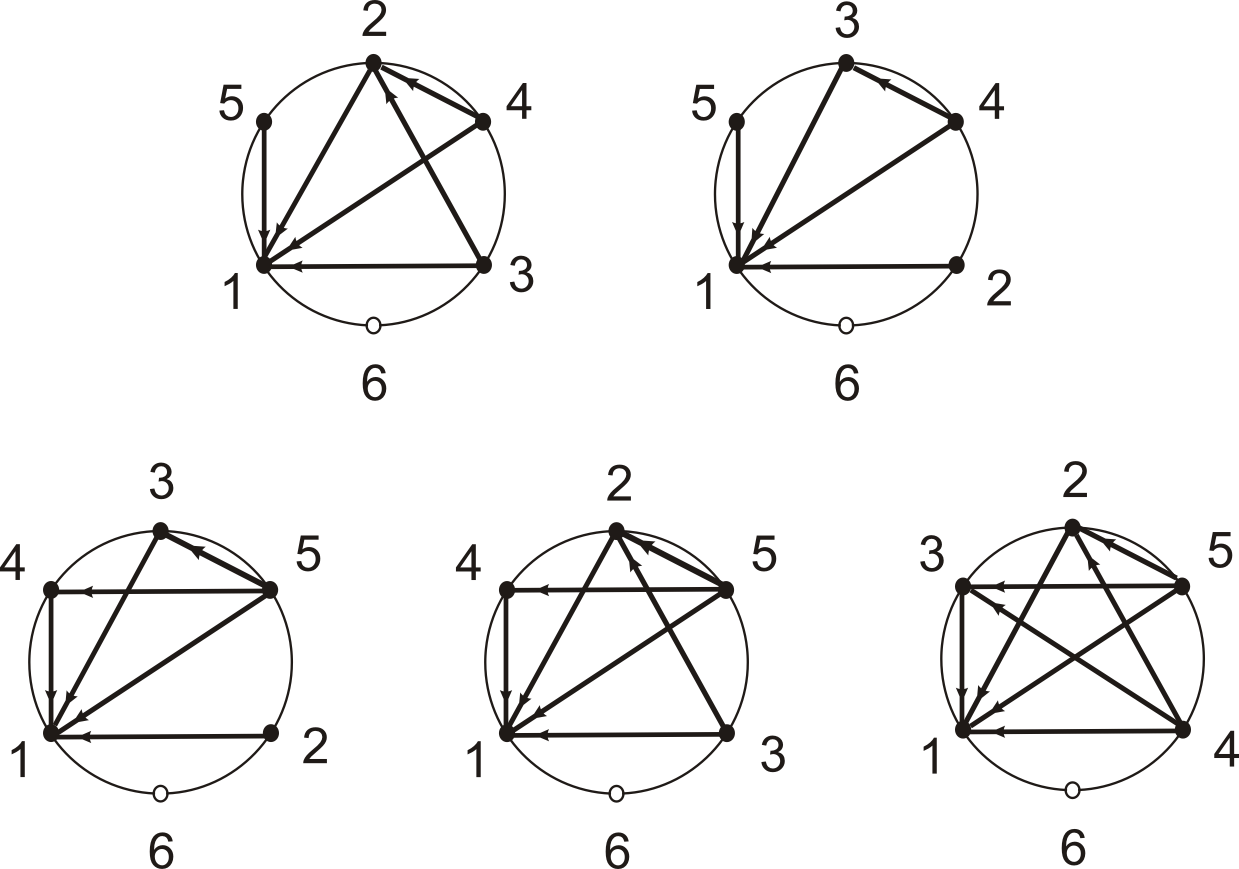
Figure 2: All arrow graphs for the six-point numerator.

The derivation just elaborated can be conveniently summarized by a set of conditions used to determine the relative positions of external lines. For simplicity we choose to represent these conditions as points on a circle. The explicit BCJ numerator will be given by the sum of contributions read off from each circle once all the integer labels have been assigned to these points.

• Step-1 To determine the $n$-point half ladder numerator $n_{1|2\dots n-1|n}$ in Cayley parametrization, we begin by drawing $n$ points on a circle, with one of them labeled by the integer $n$. We associate this special position with a hollow point to emphasize that it is off-shell continued.

• Step-2 The rest of the labels are then assigned in descending order: $n-1$, $n-2$, …, $1$, to the remaining points. We request that when every label $j$ is assigned to a position, either an odd number of unlabeled points or no unlabeled point is between $j$ and the first labeled point on the left/right hand side of $j$. When this assignment of all legs is completed, we further request discarding all graphs where integers $1$ and $n$ are not adjacent. This should give us a collection of graphs. In the case of $6$ points, the collection of all configurations satisfying the above criteria is shown in figure 1.

• Step-3 The graphs obtained through previous steps are subsequently decorated with arrows. For every labeled point $i\in\{i|1<i<n\}$ we draw arrows from $i$ to all of the labeled points $j<i$ that are on its left. Every such arrow is associated with a factor $s_{ij}$. (A demonstration of the arrow graphs at $6$ points is given by figure 2)

• Step-4 Denoting the sum of associated factors with arrows coming from point $i$ as $S_{i}=\sum\limits_{j<i,\xi_{j}<\xi_{i}}s_{ij}$, the products $\prod_{j=2}^{n-1}S_{j}$ defines the contribution of each graph. Summing over all graphs gives us the full BCJ numerator in Cayley parametrization.

Note that the conditions used to determine labels follows the operations in section 3.2 in a more or less straight forward manner. Had we artificially inserted a leg $\alpha_{1}$ between the two separated sets $\beta_{1}$ and $\beta_{2}$ on the right hand side of equations (2.12), (2.14) for the purpose of bookkeeping every time when a $U(1)$ identity or fundamental BCJ relation was used to simplify the numerator formula (3.1), the resulting sequences of legs at the end of the calculation, when placed on a circle, will be the same as those in figure 1. The rest of the rules for constructing the numerator can be easily seen by keeping track of how the Mandelstam variables were assigned.

The outcome of this graphical construction can be expressed as a succinct formula in terms of momentum kernel

$$n_{1|2,3,\dots,n-1|n}=\sum\limits_{\sigma}{\cal S}[n-1\dots 2\mid\sigma],$$ (3.29)

where $\sigma$ denote all possible permutations of $2$, $3$,…,$n-1$ satisfying the conditions in Step-2 and ${\cal S}$ is momentum kernel defined by eq. (2.3).

4 Permutation symmetric numerators in pion parametrization

In the previous sections we demonstrated how to solve the NLSM kinematic numerators via the KLT inspired approach using Cayley parametrized currents as inputs. We obtained $(n-2)!$ half ladder basis numerators with specifically chosen pairs of legs $(1,\,n)$ fixed at two ends,

$$= n_{1|2345|6},$$ (4.1)

$$= n_{1|3245|6},$$

$$\vdots$$

while all other numerators were determined by these basis half ladders through anti-symmetry and Jacobi identities. For example the following numerators are given by

$$= (-1)\times\begin{minipage}{28.45274pt} \includegraphics[width=85.35826pt]{n132456} \end{minipage}\hskip 56.9055pt$$

$$= (-1)\,n_{1|3245|6}$$

$$= (-1)\times\begin{minipage}{28.45274pt} \includegraphics[width=85.35826pt]{6pt-jacobi-tree} \end{minipage}\hskip 56.9055pt$$

$$= (-1)\times\left(\begin{minipage}{28.45274pt} \includegraphics[width=85.35826pt]{n123456} \end{minipage}\hskip 56.9055pt-\begin{minipage}{28.45274pt} \includegraphics[width=85.35826pt]{n132456} \end{minipage}\hskip 56.9055pt\right)$$

$$= (-1)\left(n_{1|2345|6}-n_{1|3245|6}\right)$$

The Jacobi identities were satisfied trivially because of the conditions we imposed to define non-basis numerators

$$\begin{minipage}{28.45274pt} \includegraphics[width=85.35826pt]{n123456} \end{minipage}\hskip 56.9055pt+\begin{minipage}{28.45274pt} \includegraphics[width=85.35826pt]{n231456} \end{minipage}\hskip 56.9055pt+\begin{minipage}{28.45274pt} \includegraphics[width=85.35826pt]{n312456} \end{minipage}\hskip 56.9055pt$$ (4.5)

$$=n_{1|2345|6}+(-1)\left(n_{1|2345|6}-n_{1|3245|6}\right)+(-1)n_{1|3245|6}$$

$$=0$$

In this approach we never needed to use the KLT inspired formulas for half ladder numerators with reference legs other than $(1,\,n)$. When appropriate propagators are included, all amplitudes in the KK sector $A(1\alpha_{2,n-1}n)$ are expressible as linear combinations of the numerators, and the numerators in turn can be spanned by half ladders $n_{1|\beta_{2,n-1}|n}$. Note however that a numerator sharing the same topology as half ladder and yet having legs other than $(1,\,n)$ fixed at two ends, for example the numerator appeared on the left hand side of equation (4), which in this picture is defined to be $(-1)\left(n_{1|2345|6}-n_{1|3245|6}\right)$, will generically be different from $n_{2|3145|6}$, the result obtained from KLT inspired formula, using legs $(2,\,n)$ as the references legs instead of $(1,\,n)$. Especially that, as we can see by directly permuting the first three legs of the explicit formula (3.13) that $n_{1|2345|6}+n_{2|3145|6}+n_{3|1245|6}$ does not give vanishing result.

This asymmetry was a result of the fact that, as was explained in Chen:2013fya , Cayley parametrization only satisfies KK relation when all external boson lines are taken on-shell. As a matter of fact it was proven in Fu:2014pya that the KLT prescribed numerators will automatically satisfies all the permutation symmetries had the KK relations been respected off-shell by the amplitudes. As an alternative, in the remaining part of this paper we will provide a more symmetric set of solutions for the NLSM numerators, where Jacobi identities and anti-symmetries between the numerators can be achieved through direct relabeling of the external boson lines. The Cayley parametrization version comparing with the later results nevertheless has the virtue of providing a much simpler prescription for the numerators.

4.1 Pion parametrization and the off-shell KK relations

In order to avoid asymmetry let us return to the original pion model, where $U[\phi]=exp\{i\phi\}$. For the purpose of discussion we would like to use the identity $\partial U^{-1}=U^{-1}\left(\partial U\right)U^{-1}$ and rewrite the chiral NLSM Lagrangian as the square of Mauerer-Cartan Form

$$S_{NLSM}[\phi] = tr\int\partial_{\mu}U^{-1}\partial^{\mu}U$$ (4.6)

$$= tr\int\left(\partial U\right)U^{-1}\left(\partial U\right)U^{-1}$$

and noting that

$$\left(\partial U\right)U^{-1}=i\left\{\left(\partial\phi\right)+\frac{(-i)}{2!}[\partial\phi,\phi]+\frac{(-i)^{2}}{3!}[[\partial\phi,\phi]\phi]+\frac{(-i)^{3}}{4!}[[[\partial\phi,\phi]\phi]\phi]+\dots\right\}$$ (4.7)

For simplicity we have chosen the pion decay constant $\sqrt{2}/F=1$. Substituting the above into the NLSM Lagrangian and expanding gives

$$\mathcal{O}(\phi^{2}) : tr\,\partial\phi\partial\phi$$ (4.8)

$$\mathcal{O}(\phi^{4}) : \frac{(-i)^{2}2}{4!}\,tr\,[[\partial\phi,\phi]\phi]\partial\phi$$ (4.9)

$$\mathcal{O}(\phi^{6}) : \frac{(-i)^{4}2}{6!}\,tr\,[[[[\partial\phi,\phi]\phi]\phi]\phi]\partial\phi$$

$$\vdots$$

$$\mathcal{O}(\phi^{2n}) : \frac{(-i)^{2n-2}2}{(2n)!}tr\,[[[[\partial\phi,\phi]\phi]\dots\phi]\partial\phi$$ (4.11)

where we have used the identity $tr(A[BC])=tr([AB]C)$ between traces to write every term in the Lagrangian as a successive commutator followed by a $\partial\phi$, before collecting them. We are also ignoring all odd number vertices because amplitudes of odd numbers of pions scattering are known to be vanishing Kampf:2013vha . Note from equations (4.8) to (4.11) that the color/flavor dependence only enters the pion amplitude through a string of structure constants

$$f^{a_{1}a_{2}e_{1}}f^{e_{1}a_{3}e_{2}}\dots f^{e_{2n-3}a_{2n-1}a_{2n}}\times\left(\partial\phi^{a_{1}}\right)\phi^{a_{2}}\phi^{a_{3}}\dots\left(\partial\phi^{a_{2n}}\right)$$ (4.12)

It is apparent that every Feynman graph in this formulation automatically carries one copy of the color structure in the form of a cubic tree, and the anti-symmetry with respect to swapping any two neighboring branches in the cubic structure guarantees KK relations between pion amplitudes even when off-shell. As we shall see in the following discussions that pion currents constructed from the vertices above can be used to determine symmetric BCJ numerators.

The Feynman rules in this formulation of the NLSM however does not directly prescribe a Jacobi satisfying BCJ numerators, as can be verified by naively identifying all the momentum dependent factors associated with each color tree as the corresponding kinematic numerator and then examine their Jacobi sum. This is because the color cubic trees are not independent, and each double-copy structure is in fact a linear combination of the Feynman graphs.

The color/flavor ordered vertices in this model are given by

$$V_{4}(1234) = \frac{(-i)^{4}2}{4!}\times\biggl{\{}\left(s_{12}+s_{23}+s_{34}+s_{41}\right)-2\left(s_{13}+s_{24}+s_{31}+s_{42}\right)+\left(s_{14}+s_{21}+s_{32}+s_{43}\right)\biggr{\}}$$

$$V_{6}(123456) = \frac{(-i)^{6}2}{6!}\times\biggl{\{}\left(s_{12}+s_{23}+s_{34}+s_{45}+s_{56}+s_{61}\right)-4\left(s_{13}+s_{24}+s_{35}+s_{46}+s_{51}+s_{62}\right)$$

$$+6\left(s_{14}+s_{25}+s_{36}+s_{41}+s_{52}+s_{63}\right)-4\left(s_{15}+s_{26}+s_{31}+s_{42}+s_{53}+s_{64}\right)$$

$$+\left(s_{16}+s_{21}+s_{32}+s_{43}+s_{54}+s_{65}\right)\biggr{\}}$$

$$\vdots$$

Generically a $2n$-vertex reads

$$V_{2n}(12\dots,2n) =\frac{(-i)^{4}2}{(2n)!}\times\biggl{\{} \left(s_{12}+s_{23}+\dots\right)-\left(\begin{array}[]{c}2n-2\\ 1\end{array}\right)\left(s_{13}+s_{24}+\dots\right)$$

$$+\left(\begin{array}[]{c}2n-22\end{array}\right)\left(s_{14}+s_{25}+\dots\right)+\dots$$

$$+\left(s_{1,2n}+s_{2,1}+\dots\right)\biggr{\}}$$

$$= \frac{(-i)^{2n}2}{(2n)!}\left\{\sum_{k=1}^{2n-1}\left((-1)^{k-1}\left(\begin{array}[]{c}2n-2\\ k-1\end{array}\right)\sum_{i=1}^{2n}s_{i,i+k}\right)\right\},$$ (4.21)

which agrees with the formula derived from a slightly different approach in Kampf:2013vha .

As a quick check we verify the $U(1)$ decoupling identity between $6$-Goldstone boson currents $J(12345)+J(21345)+J(23145)+J(23415)+J(23451)=0$, which is a limited case of the more general KK relations. The $6$-vertex contribution to the sum of amplitudes reads

$$\left(s_{16}+s_{21}+s_{32}+s_{43}+s_{54}+s_{65}\right) -4\left(s_{26}+s_{31}+s_{42}+s_{53}+s_{64}+s_{15}\right) +6\left(s_{36}+s_{14}+s_{25}\right)$$ (4.22)

$$\left(s_{26}+s_{12}+s_{31}+s_{43}+s_{54}+s_{65}\right) -4\left(s_{16}+s_{32}+s_{41}+s_{53}+s_{64}+s_{25}\right) +6\left(s_{36}+s_{24}+s_{15}\right)$$

$$\left(s_{26}+s_{32}+s_{13}+s_{41}+s_{54}+s_{65}\right) -4\left(s_{36}+s_{12}+s_{43}+s_{51}+s_{64}+s_{25}\right) +6\left(s_{16}+s_{24}+s_{35}\right)$$

$$\left(s_{26}+s_{32}+s_{43}+s_{14}+s_{51}+s_{65}\right) -4\left(s_{36}+s_{42}+s_{13}+s_{54}+s_{61}+s_{25}\right) +6\left(s_{46}+s_{21}+s_{35}\right)$$

$$\left(s_{26}+s_{32}+s_{43}+s_{54}+s_{15}+s_{61}\right) -4\left(s_{36}+s_{42}+s_{53}+s_{14}+s_{65}+s_{21}\right) +6\left(s_{46}+s_{25}+s_{31}\right)$$

We see that every $s_{i,j}$ cancel completely without referring to massless condition. A similar pairwise cancelation occurs among the $4$-vertex contribution.

4.2 BCJ relations in the pion parametrization scheme

Following the same spirit that lead to systematic construction of the numerators in Cayley parameterization, we would then like to apply KLT inspired prescription on the more symmetric pion model, in the hope that perhaps a better understanding of the algebraic structure can be obtained in this parametrization scheme, since in this picture the numerators are likely to be less obscured by generalized gauge degrees of freedoms. For this purpose we need an off-shell continuation of the BCJ relation compatible with the Feynman rules, analogous to equation (2.14). As it turns out, off-shell BCJ relation contains richer structures in the pion parametrization scheme: It is straightforward to verify using the explicit formula (LABEL:eq:4-vertex) for color/flavor ordered $4$-vertex that the BCJ sum of Goldstone boson currents at $4$-points is given by

$$s_{31}J(132)+(s_{31}+s_{32})J(123) = (s_{31}-s_{32})J(1)J(2)\times(-1)\frac{2}{4!}.$$ (4.23)

We formally retain the $2$-point currents $J(i)$ on the right hand side of the equation. This will prove helpful in recognizing the general pattern of off-shell BCJ relations in the discussion below, even though they are just a numerical factor one. At $6$-points we see that a new term is being produced. In addition to products of two sub-currents the pion parametrization scheme permits a four sub-current term,

$$s_{51}J(15234)+(s_{51}+s_{52})J(12534)+\dots+(s_{51}+s_{52}+s_{53}+s_{54})J(12345)$$ (4.24)

$$=(s_{51}-3s_{52}+3s_{53}-s_{54})J(1)J(2)J(3)J(4)\times(-1)^{2}\frac{2}{6!}\,\frac{1}{2}$$

$$+(s_{5,1+2+4}-s_{54})J(123)J(4)\times(-1)\frac{2}{4!}$$

$$+(s_{51}-s_{5,2+3+4})J(1)J(234)\times(-1)\frac{2}{4!}.$$

Repeating a similar calculation, using the explicit formula for flavor ordered $8$-vertex gives

$$s_{71}J(1723456)+\dots+(s_{71}+s_{72}+\dots+s_{76})J(1234567)$$ (4.25)

$$=(s_{71}-5s_{72}+10s_{73}-10s_{74}+5s_{75}-s_{76})J(1)J(2)J(3)J(4)J(5)J(6)\times(-1)^{3}\frac{2}{8!}\,\frac{2}{3}$$

$$+(s_{7,1+2+3}-3s_{74}+3s_{75}-s_{76})J(123)J(4)J(5)J(6)\times(-1)^{2}\frac{2}{6!}\,\frac{1}{2}$$

$$+(s_{71}-3s_{7,2+3+4}+3s_{75}-s_{76})J(1)J(234)J(5)J(6)\times(-1)^{2}\frac{2}{6!}\,\frac{1}{2}$$

$$+(s_{71}-3s_{72}+3s_{7,3+4+5}-s_{76})J(1)J(2)J(345)J(6)\times(-1)^{2}\frac{2}{6!}\,\frac{1}{2}$$

$$+(s_{71}-3s_{72}+3s_{73}-s_{7,4+5+6})J(1)J(2)J(3)J(456)\times(-1)^{2}\frac{2}{6!}\,\frac{1}{2}$$

$$+(s_{7,1+2+3+4+5}-s_{76})J(12345)J(6)\times(-1)\frac{2}{4!}$$

$$+(s_{7,1+2+3}-s_{7,4+5+6})J(123)J(456)\times(-1)\frac{2}{4!}$$

$$+(s_{71}-s_{7,2+3+4+5+6})J(1)J(23456)\times(-1)\frac{2}{4!}.$$

The pattern generalizes as we move to higher points, every time a new term

$$\Biggl{[}\sum_{k=1}^{2n-2}(-1)^{k-1}\left(\begin{array}[]{c}2n-3\\ k-1\end{array}\right)s_{2n-1,k}\Biggr{]}\,J(1)J(2)J(3)\dots J(2n-2)$$ (4.26)

enters the formula, distributing external Goldstone boson lines into $(2n-2)$ sub-currents, while all splittings appeared previously in the lower point off-shell relations carry on.

An outline of the derivations

In this paper we calculate NLSM numerators up to $8$ points, and equations (4.23), (4.24) and (4.25) together are already enough for our goal. Both the derivation details of these equations and of higher point relations follow closely to those devised for the Cayley parametrization in Chen:2013fya . So instead of elaborating, in the following we provide merely an outline of the derivation.

We note that when expanded according to Berends-Giele recursion relation, the full BCJ sum of currents can be completely broken into several BCJ sums of the lower point currents, plus BCJ sums of vertices, to which lower point currents are attached. The first part (namely the BCJ sums of lower point currents) are known if we are performing the calculation recursively. As for vertices, let us take the BCJ sum of $4$-vertices as an example. Consider the following combination:

$$s_{31}\begin{minipage}{28.45274pt} \includegraphics[width=85.35826pt]{demo1-3} \end{minipage}\hskip 56.9055pt+(s_{31}+s_{32})\begin{minipage}{28.45274pt} \includegraphics[width=85.35826pt]{demo2-3} \end{minipage}\hskip 56.9055pt$$ (4.27)

$$=\left(s_{31}V_{4}(p_{1},p_{3},p_{2},p_{4})+(s_{31}+s_{32})V_{4}(p_{1},p_{2},p_{3},p_{4})\right)\,J_{1}J_{2}\frac{1}{p_{4}^{2}}$$

Here leg $p_{3}$ is the unique leg that moves relatively to the others in the BCJ sum and is assumed to be massless, whereas the rest of the legs $p_{1}$, $p_{2}$ and $p_{4}$ connected to the same vertex $V_{4}$ are not restricted to be the same. Generically $J_{1}$ and $J_{2}$ can be sums of Feynman graphs,

(4.28)

(4.29)

To proceed we note that the BCJ sum of flavor ordered $4$-vertices can be written as the following form.

$$s_{31}V_{4}(p_{1},p_{3},p_{2},p_{4})+(s_{31}+s_{32})V_{4}(p_{1},p_{2},p_{3},p_{4})=p_{1}^{2}(s_{34}-s_{32})+p_{2}^{2}(s_{31}-s_{34})+p_{4}^{2}(s_{32}-s_{31})$$ (4.30)

Inserting the above identity into equation (4.2) produces a term proportional to $p_{1}^{2}J_{1}J_{2}\frac{1}{p_{4}^{2}}$, a term proportional to $p_{2}^{2}J_{1}J_{2}\frac{1}{p_{4}^{2}}$, and a term to $J_{1}J_{2}$. We then choose to let $p_{1}^{2}$ cancel the propagator of $J_{1}$ instead of formally keeping it as $p_{1}^{2}J_{1}$. This breaks the original $J_{1}$ into even smaller currents $V\,J_{\alpha_{1}}J_{\alpha_{2}}\dots J_{\alpha_{n1}}+\dots$. , where the ellipsis stands for the rest of the terms in (4.28). Similarly we choose to break $p_{2}^{2}J_{2}$ into $V\,J_{\beta_{1}}J_{\beta_{2}}\dots J_{\beta_{n3}}+\dots$, while letting the $J_{1}J_{2}$ term retain its present form. Note that the manipulation just described is a matter of choice, however it does affect what we get when we collect terms according to how the full current breaks into smaller ones. Repeating the same manipulation on BCJ sums of all vertices and collecting terms carrying the same product of lower-point currents, and we find that all the $1/p_{4}^{2}$ pole cancel separately in each term, yielding equations (4.23), (4.24) and (4.25).

4.3 Explicit numerators

As in the case with Cayley parametrization we follow the KLT prescription to produce NLSM numerators. At $4$ points this is simply proportional to the BCJ sum

$$\sum_{\beta\in S_{2}}S[32|\beta_{2}\beta_{3}]J(1\beta_{2}\beta_{3}4)=s_{21}\Bigl{(}s_{31}J(132)+(s_{31}+s_{32})J(123)\Bigr{)},$$ (4.31)

and the off-shell BCJ relation (4.23) translate the right hand side of the equation above into explicit formula

$$n(1234)=(-1)\frac{2}{4!}\,s_{21}(s_{31}-s_{32}).$$ (4.32)

At $6$ points we break the whole prescribed permutation sum into first a permutation sum of leg $5$ relative to the positions of the others, which is followed by the permutation of the rest of the legs. The first part is again a BCJ sum, and we use (4.24) to replace $6$ point currents with smaller ones, canceling a pole $1/k_{6}^{2}$ in the process.

$$\sum_{\beta\in S_{4}}S[5432|\beta_{2}\beta_{3}\beta_{4}\beta_{5}]J(1\beta_{2}\beta_{3}\beta_{4}\beta_{5})$$ (4.33)

$$=\sum_{\beta\in S_{3}}S[432|\beta_{2}\beta_{3}\beta_{4}]\,\Bigl{(}s_{51}J(15234)+(s_{51}+s_{52})J(12534)+\dots+(s_{51}+s_{52}+\dots+s_{54})J(12345)\Bigr{)}$$

$$=\sum_{\beta\in S_{3}}S[432|\beta_{2}\beta_{3}\beta_{4}]\,(s_{51}-3s_{5\beta_{2}}+3s_{5\beta_{3}}-s_{5\beta_{4}})J(1)J(\beta_{2})J(\beta_{3})J(\beta_{4})\times\frac{2}{6!}\,\frac{1}{2}+\dots$$

Keeping on with the same algorithm as with the Cayley parametrization and every time canceling a pole using the off-shell BCJ relation, yields the $6$-point NLSM numerator

$$n_{1|2345|6} = \frac{1}{6!}\,\Biggl{(}-3s_{12}s_{23}\Bigl{(}7s_{24}s_{25}+s_{25}s_{34}+s_{15}(s_{24}+3s_{34})+s_{24}s_{35}$$

$$-s_{34}s_{35}+s_{14}(-s_{15}+s_{25}+3s_{35}-3s_{45})+s_{24}s_{45}-3s_{34}s_{45}\Bigr{)}$$

$$+3s_{12}s_{13}\Bigl{(}-s_{24}s_{25}+3s_{25}s_{34}+s_{15}(s_{24}+s_{34})+3s_{24}s_{35}$$

$$-s_{34}s_{35}-3s_{24}s_{45}-3s_{34}s_{45}+s_{14}(7s_{15}+s_{25}+s_{35}+s_{45})\Bigr{)}\Biggr{)}$$

Expanding the above formula gives

$$n_{1|2345|6} =\frac{3}{6!} \Biggl{(}7s_{12}s_{13}s_{14}s_{15}+s_{12}s_{14}s_{15}s_{23}+s_{12}s_{13}s_{15}s_{24}-s_{12}s_{15}s_{23}s_{24}$$

$$+s_{12}s_{13}s_{14}s_{25}-s_{12}s_{14}s_{23}s_{25}-s_{12}s_{13}s_{24}s_{25}-7s_{12}s_{23}s_{24}s_{25}$$

$$+s_{12}s_{13}s_{15}s_{34}-3s_{12}s_{15}s_{23}s_{34}+3s_{12}s_{13}s_{25}s_{34}-s_{12}s_{23}s_{25}s_{34}$$

$$+s_{12}s_{13}s_{14}s_{35}-3s_{12}s_{14}s_{23}s_{35}+3s_{12}s_{13}s_{24}s_{35}-s_{12}s_{23}s_{24}s_{35}$$

$$-s_{12}s_{13}s_{34}s_{35}+s_{12}s_{23}s_{34}s_{35}+s_{12}s_{13}s_{14}s_{45}+3s_{12}s_{14}s_{23}s_{45}$$

$$-3s_{12}s_{13}s_{24}s_{45}-s_{12}s_{23}s_{24}s_{45}-3s_{12}s_{13}s_{34}s_{45}+3s_{12}s_{23}s_{34}s_{45}\Biggr{)}.$$

As was explained in the earlier discussions we are expecting the numerators just derived should satisfy permutation symmetries, since KK relations are respected off-shell in the pion parametrization scheme. To check whether this is true, first note that a $(n-2)!$ permutation symmetry involving swapping any legs other than $(1,n)$ is a built-in feature in the KLT prescription. Also note that leg $n$ in this prescription has nevertheless been made special because of the off-shell continuation, which is a price we paid to make the linear relations between amplitudes and numerators solvable. These together leave us only the relation involving swapping leg $1$ with any of the $(n-2)$ legs. The anti-symmetry between swapping $1\leftrightarrow 2$ can be readily seen in equation (4.3). In addition we check the following three identities.

$$n_{1|2345|6}+n_{2|3145|6}+n_{3|1245|6}=0,$$ (4.35)

along with

$$n_{4|2315|6} = (-1)n_{1|[[42]3]5|6}$$ (4.36)

$$= (-1)\left\{n_{1|4235|6}-n_{1|2435|6}-n_{1|3425|6}+n_{1|3245|6}\right\},$$

and

$$n_{2|3451|6} = (-1)n_{1|[[[23]4]5]|6}$$ (4.37)

$$= (-1)\left\{n_{1|2345|6}-n_{1|3245|6}-n_{1|4235|6}+n_{1|4325|6}\right.$$

$$\left.-n_{1|5234|6}+n_{1|5324|6}+n_{1|5423|6}-n_{1|5432|6}\right\}$$

and indeed, we find that they are all satisfied by the $6$-point numerator (4.3). We find similarly the permutation symmetry is also satisfied by the $4$-point numerator (4.32).

Rules for constructing Permutation symmetric numerators

Following the same manipulation we obtain the $8$-point NLSM numerator in the pion parametrization. However considering the size of the formula at $8$ points is substantially larger than the previous two lower point results we shall lay out the explicit formula in appendix A. The derivations used to systematically construct permutation symmetric numerators in this section can be summarized by the following set of rules:

1. Starting with $n-2$ integers $1$, $2$, $3$, $\dots$, $n-2$ we divide them into an even number $2m$ of ordered sets, with only an odd number of integers allowed in every set. In addition, integer $1$ must be assigned to the first set, and the ordering within each set does not matter. For every such configuration we write down a factor $(\sum_{k=1}^{2m-1}(-1)^{k-1}\left(\begin{array}[]{c}2m-1\\ k-1\end{array}\right)s_{n-1,\beta_{k}})$, where $\beta_{k}$ is the sum of momenta in set $k$. For example

   $$(134)\,(5)\,(6)\,(2)$$ (4.38)

   is an acceptable configuration for assigning $1$, $2$, $3$, $4$, $5$, $6$ into four distinctive sets. For this configuration we write down a factor $(s_{7,1+3+4}-3s_{7,5}+3s_{7,6}-s_{7,2})$.

2. We then inspect the integers assigned into sets one by one in descending order, if the largest integer $j$ has been assigned alone into one of the sets, we multiply the original result by a factor $(s_{j,1}+\sum_{q\in\text{sets to the left of }j}\,\theta(j,q)s_{j,q})$, where $\theta(j,q)=1$ if $q<j$, and $\theta(j,q)=0$ if otherwise. To put it in plain words, we consider all integers $q$’s that are on the left of $j$. Whenever they are smaller than $j$ we include a factor $s_{j,q}$ into the sum. In the example above, since integer $6$ is assigned alone we multiply the original result by $(s_{6,1}+s_{6,3}+s_{6,4}+s_{6,5})$.

3. Turning to the next largest integer, if it is again alone we repeat step two; if it is not alone, we remove this integer and divide the rest in the same set according to step one. In this example number $4$ resides in the first set with $1$, $3$. We therefore remove integer $4$ and then divide, producing

   $$(1)(3)\,(5)\,(6)\,(2)$$ (4.39)

   Repeating the above two steps for all integers in descending order until all integers are considered and all reside in different sets all by themselves, the sum of products of factors we obtain following these steps for all allowed configurations is the $n$-point numerator in pion parametrization.

Remarks

We conclude this section with a few remarks. At first sight the explicit results we presented here and in the appendix may contain an intimidatingly large number of terms, but in fact they are much smaller than they could be. Note that for example the $6$-point numerator has the dimension of $(s_{i,j})^{4}$, and we have $C^{6}_{2}=15$ such Mandelstam variables, together there are $15^{4}\sim 5\times 10^{4}$ terms that match the dimension. Instead we only have $24$ terms that appeared in equation (4.3), all assuming the following form

$$s_{i,2}\,s_{j,3}\,s_{k,4}\,s_{l,5}$$ (4.40)

with $i$, $j$, $k$, $l$ only permitted to be smaller than the label of the legs they are paired with: $l=\{1,2,3,4\}$, $k=\{1,2,3\}$, $\dots$ etc. The fact that this pattern is general can be seen from the summarizing rules for constructing the numerators. Generically there are $(n-2)!$ terms for an $n$-point numerator $n(123\dots n)$. At the moment it is not clear whether there is an algebraic interpretation or deeper understanding to the structure observed, and we leave the exploration of these questions to future works.

5 Conclusion

From the defining Lagrangian of the theory, in this paper we have derived the BCJ numerators of the non-linear sigma model in two different parametrization schemes. We performed the calculation in the one leg off-shell continued scenario, where the propagator matrix can be inverted, and the numerator expressible as the permutation sum of currents multiplied by momentum kernel Mafra:2016ltu . A BCJ sum was then identified from the full expression and can be subsequently simplified using the BCJ relation between currents, similarly to the procedure demonstrated for color-dressed scalar theory in Du:2011js . To proceed any step further, however, one needs to show that the explicit form of the BCJ relation produces terms that can be again packed into BCJ sums. And indeed, we found this is true in both the Cayley and pion parametrizations, and this procedure was then iterated until the numerator formulas contained only Mandelstam variables. We calculated the numerators up to $8$-points. For higher multiplicities, in both parametrization schemes we summarize this procedure as a set of construction rules that applies generically. In the case of Cayley parametriztion we found that the result can be further organized into a simple formula in terms of momentum kernel.

A perhaps most natural question brought about by these findings would then be that whether an actual algebra can be found that explains the NLSM numerators. We note that, provided there is enough degrees of freedom, in principle it is possible to write down an ansatz as a string of structure constants of the most general tensorial local generators and match the explicit numerators order by order. Alternatively, one can also obtain BCJ counterpart of traces using for example the algorithm presented in Bern:2011ia ; Du:2013sha and try to identify patterns. It is still not clear at the moment whether any of these approaches would lead to simple results. It would be desirable to have a deeper understanding to the origin of the BCJ relations observed in the NLSM.

Appendix A $8$-point permutation symmetric numerator

In this appendix we list the result for $8$-point numerator in pion parametrization.

$$n_{1|234567|8}=\sum_{\beta}{\cal S}[765432|\beta_{2,7}]\,J(1\beta_{2,7}8)$$ (A.1)

$$=(-1)^{3} \sum\limits_{\beta}S[65432|\beta_{2,6}] \left(\frac{2}{8!}\right)\frac{2}{3}(s_{7,1}-5s_{7,\beta_{2}}+10s_{7,\beta_{3}}-10s_{7,\beta_{4}}+5s_{7,\beta_{5}}-s_{7,\beta_{6}})$$

$$+(-1)^{3} \sum\limits_{\beta}S[5432|\beta_{2,5}] \Biggl{(}\left(\frac{2}{4!}\right)\left(\frac{2}{6!}\right)\frac{1}{2}(s_{6,1}-s_{6,\beta_{2}})(s_{7,1+\beta_{2}+6}-3s_{7,\beta_{3}}+3s_{7,\beta_{4}}-s_{7,\beta_{5}})$$

$$+\left(\frac{2}{4!}\right)\left(\frac{2}{6!}\right)\frac{1}{2}(s_{6,\beta_{2}}-s_{6,\beta_{3}})(s_{7,1}-3s_{7,6+\beta_{2}+\beta_{3}}+3s_{7,\beta_{4}}-s_{7,\beta_{5}})$$

$$+\left(\frac{2}{4!}\right)\left(\frac{2}{6!}\right)\frac{1}{2}(s_{6,\beta_{3}}-s_{6,\beta_{4}})(s_{7,1}-3s_{7,\beta_{2}}+3s_{7,6+\beta_{3}+\beta_{4}}-s_{7,\beta_{5}})$$

$$+\left(\frac{2}{4!}\right)\left(\frac{2}{6!}\right)\frac{1}{2}(s_{6,\beta_{4}}-s_{6,\beta_{5}})(s_{7,1}-3s_{7,\beta_{2}}+3s_{7,\beta_{3}}-s_{7,6+\beta_{4}+\beta_{5}})$$

$$+\left(\frac{2}{4!}\right)\left(\frac{2}{6!}\right)\frac{1}{2}(s_{6,1}-3s_{6,\beta_{2}}+3s_{6,\beta_{3}}-s_{6,\beta_{4}})(s_{7,1+\beta_{2}+\beta_{3}+\beta_{4}}-s_{7,\beta_{5}})$$

$$+\left(\frac{2}{4!}\right)\left(\frac{2}{6!}\right)\frac{1}{2}(s_{6,\beta_{2}}-3s_{6,\beta_{3}}+3s_{6,\beta_{4}}-s_{6,\beta_{5}})(s_{7,1}-s_{7,6+\beta_{2}+\beta_{3}+\beta_{4}+\beta_{5}})\Biggr{)}$$

$$+(-1)^{3} \sum\limits_{\beta}S[432|\beta_{2,4}] \Biggl{(}\left(\frac{2}{4!}\right)\left(\frac{2}{6!}\right)\frac{1}{2}(s_{5,1}-s_{5,\beta_{2}})s_{6,1+5+\beta_{2}}(s_{7,1+5+\beta_{2}}-3s_{7,6}+3s_{7,\beta_{3}}-s_{7,\beta_{4}})$$

$$+\left(\frac{2}{4!}\right)\left(\frac{2}{6!}\right)\frac{1}{2}(s_{5,1}-s_{5,\beta_{2}})s_{6,1+5+\beta_{2}+\beta_{3}}(s_{7,1+5+\beta_{2}}-3s_{7,\beta_{3}}+3s_{7,6}-s_{7,\beta_{4}})$$

$$+\left(\frac{2}{4!}\right)\left(\frac{2}{6!}\right)\frac{1}{2}(s_{5,1}-s_{5,\beta_{2}})s_{6,1+5+\beta_{2}+\beta_{3}+\beta_{4}}(s_{7,1+5+\beta_{2}}-3s_{7,\beta_{3}}+3s_{7,\beta_{4}}-s_{7,6})$$

$$+\left(\frac{2}{4!}\right)\left(\frac{2}{6!}\right)\frac{1}{2}(s_{5,\beta_{2}}-s_{5,\beta_{3}})s_{6,1+5+\beta_{2}+\beta_{3}}(s_{7,1}-3s_{7,5+\beta_{2}+\beta_{3}}+3s_{7,6}-s_{7,4})$$

$$+\left(\frac{2}{4!}\right)\left(\frac{2}{6!}\right)\frac{1}{2}(s_{5,\beta_{2}}-s_{5,\beta_{3}})s_{6,1+5+\beta_{2}+\beta_{3}+\beta_{4}}(s_{7,1}-3s_{7,5+\beta_{2}+\beta_{3}}+3s_{7,\beta_{4}}-s_{7,6})$$

$$+\left(\frac{2}{4!}\right)\left(\frac{2}{6!}\right)\frac{1}{2}(s_{5,\beta_{2}}-s_{5,\beta_{3}})s_{6,1}(s_{7,1}-3s_{7,6}+3s_{7,5+\beta_{2}+\beta_{3}}-s_{7,\beta_{4}})$$

$$+\left(\frac{2}{4!}\right)\left(\frac{2}{6!}\right)\frac{1}{2}(s_{5,\beta_{3}}-s_{5,\beta_{4}})s_{6,1+\beta_{2}+\beta_{3}+\beta_{4}+5}(s_{7,1}-3s_{7,\beta_{2}}+3s_{7,5+\beta_{3}+\beta_{4}}-s_{7,6})$$

$$+\left(\frac{2}{4!}\right)\left(\frac{2}{6!}\right)\frac{1}{2}(s_{5,\beta_{3}}-s_{5,\beta_{4}})s_{6,1}(s_{7,1}-3s_{7,6}+3s_{7,\beta_{2}}-s_{7,5+\beta_{3}+\beta_{4}})$$

$$+\left(\frac{2}{4!}\right)\left(\frac{2}{6!}\right)\frac{1}{2}(s_{5,\beta_{3}}-s_{5,\beta_{4}})s_{6,1+\beta_{2}}(s_{7,1}-3s_{7,\beta_{2}}+3s_{7,6}-s_{7,5+\beta_{3}+\beta_{4}})$$

$$+\left(\frac{2}{4!}\right)\left(\frac{2}{6!}\right)\frac{1}{2}(s_{5,1}-3s_{5,\beta_{2}}+3s_{5,\beta_{3}}-s_{s,\beta_{4}})s_{6,1+5+\beta_{2}+\beta_{3}+\beta_{4}}(s_{7,1+5+\beta_{2}+\beta_{3}+\beta_{4}}-s_{7,6})$$

$$+\left(\frac{2}{4!}\right)^{3}(s_{7,1+\beta_{2}+6}-s_{7,\beta_{3}+\beta_{4}+5})(s_{6,1}-s_{6,\beta_{2}})(s_{5,\beta_{3}}-s_{5,\beta_{4}})$$

$$+\left(\frac{2}{4!}\right)^{3}(s_{7,1+\beta_{2}+5}-s_{7,\beta_{3}+\beta_{4}+6})(s_{6,\beta_{3}}-s_{6,\beta_{4}})(s_{5,1}-s_{5,2})\Biggr{)}$$

$$+(-1)^{3} \sum\limits_{\beta}S[32|\beta_{2,3}] \Biggl{(}\left(\frac{2}{4!}\right)\left(\frac{2}{6!}\right)\frac{1}{2}(s_{4,1}-s_{4,\beta_{2}})s_{5,1+4+\beta_{2}}s_{6,1+4+\beta_{2}}(s_{7,1+4+\beta_{2}}-3s_{7,6}+3s_{7,5}-s_{7,\beta_{3}})$$

$$+\left(\frac{2}{4!}\right)\left(\frac{2}{6!}\right)\frac{1}{2}(s_{4,1}-s_{4,\beta_{2}})s_{5,1+4+\beta_{2}+\beta_{3}}s_{6,1+4+\beta_{2}}(s_{7,1+4+\beta_{2}}-3s_{7,6}+3s_{7,\beta_{3}}-s_{7,5})$$

$$+\left(\frac{2}{4!}\right)\left(\frac{2}{6!}\right)\frac{1}{2}(s_{4,1}-s_{4,\beta_{2}})s_{5,1+4+\beta_{2}}s_{6,1+4+\beta_{2}+5}(s_{7,1+4+\beta_{2}}-3s_{7,5}+3s_{7,6}-s_{7,\beta_{3}})$$

$$+\left(\frac{2}{4!}\right)\left(\frac{2}{6!}\right)\frac{1}{2}(s_{4,1}-s_{4,\beta_{2}})s_{5,1+4+\beta_{2}+\beta_{3}}s_{6,1+4+\beta_{2}+\beta_{3}}(s_{7,1+4+\beta_{2}}-3s_{7,\beta_{3}}+3s_{7,6}-s_{7,5})$$

$$+\left(\frac{2}{4!}\right)\left(\frac{2}{6!}\right)\frac{1}{2}(s_{4,1}-s_{4,\beta_{2}})s_{5,1+4+\beta_{2}}s_{6,1+4+\beta_{2}+5+\beta_{3}}(s_{7,1+4+\beta_{2}}-3s_{7,5}+3s_{7,\beta_{3}}-s_{7,6})$$

$$+\left(\frac{2}{4!}\right)\left(\frac{2}{6!}\right)\frac{1}{2}(s_{4,1}-s_{4,\beta_{2}})s_{5,1+4+\beta_{2}+\beta_{3}}s_{6,1+4+\beta_{2}+\beta_{3}+5}(s_{7,1+4+\beta_{2}}-3s_{7,\beta_{3}}+3s_{7,5}-s_{7,6})$$

$$+\left(\frac{2}{4!}\right)\left(\frac{2}{6!}\right)\frac{1}{2}(s_{4,\beta_{2}}-s_{4,\beta_{3}})s_{5,1+4+\beta_{2}+\beta_{3}}s_{6,1+4+\beta_{2}+\beta_{3}}(s_{7,1}-3s_{7,4+\beta_{2}+\beta_{3}}+3s_{7,6}-s_{7,5})$$

$$+\left(\frac{2}{4!}\right)\left(\frac{2}{6!}\right)\frac{1}{2}(s_{4,\beta_{2}}-s_{4,\beta_{3}})s_{5,1+4+\beta_{2}+\beta_{3}}s_{6,1+4+\beta_{2}+\beta_{3}+5}(s_{7,1}-3s_{7,4+\beta_{2}+\beta_{3}}+3s_{7,5}-s_{7,6})$$

$$+\left(\frac{2}{4!}\right)\left(\frac{2}{6!}\right)\frac{1}{2}(s_{4,\beta_{2}}-s_{4,\beta_{3}})s_{5,1+4+\beta_{2}+\beta_{3}}s_{6,1}(s_{7,1}-3s_{7,6}+3s_{7,4+\beta_{2}+\beta_{3}}-s_{7,5})$$

$$+\left(\frac{2}{4!}\right)\left(\frac{2}{6!}\right)\frac{1}{2}(s_{4,\beta_{2}}-s_{4,\beta_{3}})s_{5,1}s_{6,1+5+4+\beta_{2}+\beta_{3}}(s_{7,1}-3s_{7,5}+3s_{7,4+\beta_{2}+\beta_{3}}-s_{7,6})$$

$$+\left(\frac{2}{4!}\right)\left(\frac{2}{6!}\right)\frac{1}{2}(s_{4,\beta_{2}}-s_{4,\beta_{3}})s_{5,1}s_{6,1}(s_{7,1}-3s_{7,6}+3s_{7,5}-s_{7,4+\beta_{2}+\beta_{3}})$$

$$+\left(\frac{2}{4!}\right)\left(\frac{2}{6!}\right)\frac{1}{2}(s_{4,\beta_{2}}-s_{4,\beta_{3}})s_{5,1}s_{6,1+5}(s_{7,1}-3s_{7,5}+3s_{7,6}-s_{7,4+\beta_{2}+\beta_{3}})$$

$$+\left(\frac{2}{4!}\right)^{3}(s_{4,1}-s_{4,\beta_{2}})(s_{5,1+4+\beta_{2}}-s_{5,\beta_{3}})s_{6,1+5+4+\beta_{2}+\beta_{3}}(s_{7,6}-s_{7,1+5+4+\beta_{2}\beta_{3}})$$

$$+\left(\frac{2}{4!}\right)^{3}(s_{4,\beta_{2}}-s_{4,\beta_{3}})(s_{5,1}-s_{5,4+\beta_{2}+\beta_{3}})s_{6,1+5+4+\beta_{2}+\beta_{3}}(s_{7,6}-s_{7,1+5+4+\beta_{2}\beta_{3}})$$

$$+\left(\frac{2}{4!}\right)^{3}(s_{7,1+5+6}-s_{7,\beta_{2}+\beta_{3}+4})(s_{6,1}-s_{6,5})s_{5,1}(s_{4,\beta_{2}}-s_{4,\beta_{3}})$$

$$+\left(\frac{2}{4!}\right)^{3}(s_{7,1+\beta_{2}+4}-s_{7,5+\beta_{3}+6})(s_{6,5}-s_{6,\beta_{3}})s_{5,1+\beta_{2}+4}(s_{4,1}-s_{4,\beta_{2}})$$

$$+\left(\frac{2}{4!}\right)^{3}(s_{7,1+\beta_{2}+4}-s_{7,\beta_{3}+5+6})(s_{6,\beta_{3}}-s_{6,5})s_{5,1+\beta_{2}+4+\beta_{3}}(s_{4,1}-s_{4,\beta_{2}})\Biggr{)}$$

$$+(-1)^{3} S[2|2] \Biggl{(}\left(\frac{2}{4!}\right)\left(\frac{2}{6!}\right)\frac{1}{2}(s_{3,1}-s_{3,2})s_{4,1+2+3}s_{5,1+2+3}s_{6,1+2+3}(s_{7,1+2+3}-3s_{7,6}+3s_{7,5}-s_{7,4})$$

$$+\left(\frac{2}{4!}\right)\left(\frac{2}{6!}\right)\frac{1}{2}(s_{3,1}-s_{3,2})s_{4,1+2+3}s_{5,1+2+3}s_{6,1+2+3}(s_{7,1+2+3}-3s_{7,6}+3s_{7,4}-s_{7,5})$$

$$+\left(\frac{2}{4!}\right)\left(\frac{2}{6!}\right)\frac{1}{2}(s_{3,1}-s_{3,2})s_{4,1+2+3}s_{5,1+2+3}s_{6,1+2+3+5}(s_{7,1+2+3}-3s_{7,5}+3s_{7,6}-s_{7,4})$$

$$+\left(\frac{2}{4!}\right)\left(\frac{2}{6!}\right)\frac{1}{2}(s_{3,1}-s_{3,2})s_{4,1+2+3}s_{5,1+2+3+4}s_{6,1+2+3+4}(s_{7,1+2+3}-3s_{7,4}+3s_{7,6}-s_{7,5})$$

$$+\left(\frac{2}{4!}\right)\left(\frac{2}{6!}\right)\frac{1}{2}(s_{3,1}-s_{3,2})s_{4,1+2+3}s_{5,1+2+3}s_{6,1+2+3+5+4}(s_{7,1+2+3}-3s_{7,5}+3s_{7,4}-s_{7,6})$$

$$+\left(\frac{2}{4!}\right)\left(\frac{2}{6!}\right)\frac{1}{2}(s_{3,1}-s_{3,2})s_{4,1+2+3}s_{5,1+2+3+4}s_{6,1+2+3+4+5}(s_{7,1+2+3}-3s_{7,4}+3s_{7,5}-s_{7,6})$$

$$+\left(\frac{2}{4!}\right)^{3}(s_{3,1}-s_{3,2})s_{4,1+2+3}(s_{5,1+2+3}-s_{5,4})s_{6,1+5+2+3+4}(s_{7,1+5+2+3+4}-s_{7,6})$$

$$+\left(\frac{2}{4!}\right)^{3}(s_{7,1+2+3}-s_{7,5+4+6})(s_{6,5}-s_{6,4})s_{5,1+2+3}s_{4,1+2+3}(s_{3,1}-s_{3,2})$$

$$+\left(\frac{2}{4!}\right)^{3}(s_{7,1+2+3}-s_{7,4+5+6})(s_{6,4}-s_{6,5})s_{5,1+2+3+4}s_{4,1+2+3}(s_{3,1}-s_{3,2})\Biggr{)}$$

References

• (1) Z. Bern, J. J. M. Carrasco and H. Johansson, “New Relations for Gauge-Theory Amplitudes,” Phys. Rev. D 78 (2008) 085011 doi:10.1103/PhysRevD.78.085011 [arXiv:0805.3993 [hep-ph]].
• (2) R. Monteiro and D. O’Connell, “The Kinematic Algebra From the Self-Dual Sector,” JHEP 1107 (2011) 007 doi:10.1007/JHEP07(2011)007 [arXiv:1105.2565 [hep-th]].
• (3) B. Feng, R. Huang and Y. Jia, “Gauge Amplitude Identities by On-shell Recursion Relation in S-matrix Program,” Phys. Lett. B 695 (2011) 350 doi:10.1016/j.physletb.2010.11.011 [arXiv:1004.3417 [hep-th]].
• (4) F. Cachazo, “Fundamental BCJ Relation in N=4 SYM From The Connected Formulation,” arXiv:1206.5970 [hep-th].
• (5) S. Stieberger, “Open & Closed vs. Pure Open String Disk Amplitudes,” arXiv:0907.2211 [hep-th].
• (6) N. E. J. Bjerrum-Bohr, P. H. Damgaard and P. Vanhove, “Minimal Basis for Gauge Theory Amplitudes,” Phys. Rev. Lett.  103 (2009) 161602 doi:10.1103/PhysRevLett.103.161602 [arXiv:0907.1425 [hep-th]].
• (7) Z. Bern, J. J. M. Carrasco and H. Johansson, “Perturbative Quantum Gravity as a Double Copy of Gauge Theory,” Phys. Rev. Lett.  105 (2010) 061602 doi:10.1103/PhysRevLett.105.061602 [arXiv:1004.0476 [hep-th]].
• (8) Z. Bern, T. Dennen, Y. t. Huang and M. Kiermaier, “Gravity as the Square of Gauge Theory,” Phys. Rev. D 82 (2010) 065003 doi:10.1103/PhysRevD.82.065003 [arXiv:1004.0693 [hep-th]].
• (9) H. Kawai, D. Lewellen and H. Tye, ”A Relation Betwwen Tree Amplitudes of Closed and Open Strings”, Nucl.Phys.B269 (1986)1.
• (10) M. Kiermaier, Gravity as the Square of Gauge Theory, talk at Amplitudes 2010, May 2010 at QMUL, London, UK. http://www.strings.ph.qmul.ac.uk/~theory/Amplitudes2010/Talks/MK2010.pdf
• (11) Z. Bern, J. J. M. Carrasco, L. J. Dixon, H. Johansson and R. Roiban, “Simplifying Multiloop Integrands and Ultraviolet Divergences of Gauge Theory and Gravity Amplitudes,” Phys. Rev. D 85 (2012) 105014 doi:10.1103/PhysRevD.85.105014 [arXiv:1201.5366 [hep-th]].
• (12) Z. Bern, S. Davies and T. Dennen, “The Ultraviolet Structure of Half-Maximal Supergravity with Matter Multiplets at Two and Three Loops,” Phys. Rev. D 88 (2013) 065007 doi:10.1103/PhysRevD.88.065007 [arXiv:1305.4876 [hep-th]].
• (13) Z. Bern, S. Davies and T. Dennen, “Enhanced ultraviolet cancellations in $\mathcal{N}=5$ supergravity at four loops,” Phys. Rev. D 90 (2014) no.10, 105011 doi:10.1103/PhysRevD.90.105011 [arXiv:1409.3089 [hep-th]].
• (14) C. R. Mafra and O. Schlotterer, “Multiparticle SYM equations of motion and pure spinor BRST blocks,” JHEP 1407 (2014) 153 doi:10.1007/JHEP07(2014)153 [arXiv:1404.4986 [hep-th]].
• (15) C. R. Mafra and O. Schlotterer, “Towards one-loop SYM amplitudes from the pure spinor BRST cohomology,” Fortsch. Phys.  63 (2015) no.2, 105 doi:10.1002/prop.201400076 [arXiv:1410.0668 [hep-th]].
• (16) C. R. Mafra and O. Schlotterer, “Two-loop five-point amplitudes of super Yang-Mills and supergravity in pure spinor superspace,” JHEP 1510 (2015) 124 doi:10.1007/JHEP10(2015)124 [arXiv:1505.02746 [hep-th]].
• (17) R. H. Boels, R. S. Isermann, R. Monteiro and D. O’Connell, “Colour-Kinematics Duality for One-Loop Rational Amplitudes,” JHEP 1304 (2013) 107 doi:10.1007/JHEP04(2013)107 [arXiv:1301.4165 [hep-th]].
• (18) J. J. Carrasco and H. Johansson, “Five-Point Amplitudes in N=4 Super-Yang-Mills Theory and N=8 Supergravity,” Phys. Rev. D 85 (2012) 025006 doi:10.1103/PhysRevD.85.025006 [arXiv:1106.4711 [hep-th]].
• (19) N. E. J. Bjerrum-Bohr, T. Dennen, R. Monteiro and D. O’Connell, “Integrand Oxidation and One-Loop Colour-Dual Numerators in N=4 Gauge Theory,” JHEP 1307 (2013) 092 doi:10.1007/JHEP07(2013)092 [arXiv:1303.2913 [hep-th]].
• (20) J. J. M. Carrasco, M. Chiodaroli, M. Günaydin and R. Roiban, “One-loop four-point amplitudes in pure and matter-coupled N ¡= 4 supergravity,” JHEP 1303 (2013) 056 doi:10.1007/JHEP03(2013)056 [arXiv:1212.1146 [hep-th]].
• (21) Z. Bern, S. Davies, T. Dennen, Y. t. Huang and J. Nohle, “Color-Kinematics Duality for Pure Yang-Mills and Gravity at One and Two Loops,” Phys. Rev. D 92 (2015) no.4, 045041 doi:10.1103/PhysRevD.92.045041 [arXiv:1303.6605 [hep-th]].
• (22) J. Nohle, “Color-Kinematics Duality in One-Loop Four-Gluon Amplitudes with Matter,” Phys. Rev. D 90 (2014) no.2, 025020 doi:10.1103/PhysRevD.90.025020 [arXiv:1309.7416 [hep-th]].
• (23) A. Ochirov and P. Tourkine, “BCJ duality and double copy in the closed string sector,” JHEP 1405 (2014) 136 doi:10.1007/JHEP05(2014)136 [arXiv:1312.1326 [hep-th]].
• (24) M. Chiodaroli, Q. Jin and R. Roiban, “Color/kinematics duality for general abelian orbifolds of N=4 super Yang-Mills theory,” JHEP 1401 (2014) 152 doi:10.1007/JHEP01(2014)152 [arXiv:1311.3600 [hep-th]].
• (25) M. Chiodaroli, M. Günaydin, H. Johansson and R. Roiban, “Scattering amplitudes in $\mathcal{N}=2$ Maxwell-Einstein and Yang-Mills/Einstein supergravity,” JHEP 1501 (2015) 081 doi:10.1007/JHEP01(2015)081 [arXiv:1408.0764 [hep-th]].
• (26) E. Y. Yuan, “Virtual Color-Kinematics Duality: 6-pt 1-Loop MHV Amplitudes,” JHEP 1305 (2013) 070 doi:10.1007/JHEP05(2013)070 [arXiv:1210.1816 [hep-th]].
• (27) S. Oxburgh and C. D. White, “BCJ duality and the double copy in the soft limit,” JHEP 1302 (2013) 127 doi:10.1007/JHEP02(2013)127 [arXiv:1210.1110 [hep-th]].
• (28) R. Saotome and R. Akhoury, “Relationship Between Gravity and Gauge Scattering in the High Energy Limit,” JHEP 1301 (2013) 123 doi:10.1007/JHEP01(2013)123 [arXiv:1210.8111 [hep-th]].
• (29) H. Elvang and Y. t. Huang, “Scattering Amplitudes,” arXiv:1308.1697 [hep-th].
• (30) J. J. M. Carrasco, “Gauge and Gravity Amplitude Relations,” doi:10.1142/9789814678766_0011 arXiv:1506.00974 [hep-th].
• (31) N. E. J. Bjerrum-Bohr, P. H. Damgaard, R. Monteiro and D. O’Connell, “Algebras for Amplitudes,” JHEP 1206 (2012) 061 doi:10.1007/JHEP06(2012)061 [arXiv:1203.0944 [hep-th]].
• (32) F. Cachazo, S. He and E. Y. Yuan, “Scattering equations and Kawai-Lewellen-Tye orthogonality,” Phys. Rev. D 90 (2014) no.6, 065001 doi:10.1103/PhysRevD.90.065001 [arXiv:1306.6575 [hep-th]].
• (33) F. Cachazo, S. He and E. Y. Yuan, “Scattering of Massless Particles in Arbitrary Dimensions,” Phys. Rev. Lett.  113 (2014) no.17, 171601 doi:10.1103/PhysRevLett.113.171601 [arXiv:1307.2199 [hep-th]].
• (34) F. Cachazo, S. He and E. Y. Yuan, “Scattering of Massless Particles: Scalars, Gluons and Gravitons,” JHEP 1407 (2014) 033 doi:10.1007/JHEP07(2014)033 [arXiv:1309.0885 [hep-th]].
• (35) R. Monteiro and D. O’Connell, “The Kinematic Algebras from the Scattering Equations,” JHEP 1403 (2014) 110 doi:10.1007/JHEP03(2014)110 [arXiv:1311.1151 [hep-th]].
• (36) S. He, R. Monteiro and O. Schlotterer, “String-inspired BCJ numerators for one-loop MHV amplitudes,” JHEP 1601 (2016) 171 doi:10.1007/JHEP01(2016)171 [arXiv:1507.06288 [hep-th]].
• (37) H. Johansson and A. Ochirov, “Color-Kinematics Duality for QCD Amplitudes,” JHEP 1601 (2016) 170 doi:10.1007/JHEP01(2016)170 [arXiv:1507.00332 [hep-ph]].
• (38) T. Bargheer, S. He and T. McLoughlin, “New Relations for Three-Dimensional Supersymmetric Scattering Amplitudes,” Phys. Rev. Lett.  108 (2012) 231601 doi:10.1103/PhysRevLett.108.231601 [arXiv:1203.0562 [hep-th]].
• (39) Y. t. Huang and H. Johansson, “Equivalent D=3 Supergravity Amplitudes from Double Copies of Three-Algebra and Two-Algebra Gauge Theories,” Phys. Rev. Lett.  110 (2013) 171601 doi:10.1103/PhysRevLett.110.171601 [arXiv:1210.2255 [hep-th]].
• (40) R. Monteiro, D. O’Connell and C. D. White, “Black holes and the double copy,” JHEP 1412 (2014) 056 doi:10.1007/JHEP12(2014)056 [arXiv:1410.0239 [hep-th]].
• (41) A. Luna, R. Monteiro, D. O’Connell and C. D. White, “The classical double copy for Taub-NUT spacetime,” Phys. Lett. B 750 (2015) 272 doi:10.1016/j.physletb.2015.09.021 [arXiv:1507.01869 [hep-th]].
• (42) H. Johansson and A. Ochirov, “Pure Gravities via Color-Kinematics Duality for Fundamental Matter,” JHEP 1511 (2015) 046 doi:10.1007/JHEP11(2015)046 [arXiv:1407.4772 [hep-th]].
• (43) T. Sondergaard, “New Relations for Gauge-Theory Amplitudes with Matter,” Nucl. Phys. B 821 (2009) 417 doi:10.1016/j.nuclphysb.2009.07.002 [arXiv:0903.5453 [hep-th]].
• (44) S. Weinzierl, “Fermions and the scattering equations,” JHEP 1503 (2015) 141 doi:10.1007/JHEP03(2015)141 [arXiv:1412.5993 [hep-th]].
• (45) S. G. Naculich, “Scattering equations and BCJ relations for gauge and gravitational amplitudes with massive scalar particles,” JHEP 1409 (2014) 029 doi:10.1007/JHEP09(2014)029 [arXiv:1407.7836 [hep-th]].
• (46) S. G. Naculich, “CHY representations for gauge theory and gravity amplitudes with up to three massive particles,” JHEP 1505 (2015) 050 doi:10.1007/JHEP05(2015)050 [arXiv:1501.03500 [hep-th]].
• (47) M. Chiodaroli, M. Gunaydin, H. Johansson and R. Roiban, “Spontaneously Broken Yang-Mills-Einstein Supergravities as Double Copies,” arXiv:1511.01740 [hep-th].
• (48) K. Kampf, J. Novotny and J. Trnka, “Tree-level Amplitudes in the Nonlinear Sigma Model,” JHEP 1305 (2013) 032 doi:10.1007/JHEP05(2013)032 [arXiv:1304.3048 [hep-th]].
• (49) G. Chen and Y. J. Du, “Amplitude Relations in Non-linear Sigma Model,” JHEP 1401 (2014) 061 doi:10.1007/JHEP01(2014)061 [arXiv:1311.1133 [hep-th]].
• (50) G. Chen, Y. J. Du, S. Li and H. Liu, “Note on off-shell relations in nonlinear sigma model,” JHEP 1503 (2015) 156 doi:10.1007/JHEP03(2015)156 [arXiv:1412.3722 [hep-th]].
• (51) Y. J. Du, B. Feng and C. H. Fu, “BCJ Relation of Color Scalar Theory and KLT Relation of Gauge Theory,” JHEP 1108 (2011) 129 doi:10.1007/JHEP08(2011)129 [arXiv:1105.3503 [hep-th]].
• (52) Z. Bern, “Perturbative quantum gravity and its relation to gauge theory,” Living Rev. Rel.  5 (2002) 5 doi:10.12942/lrr-2002-5 [gr-qc/0206071].
• (53) Z. Bern, A. De Freitas and H. L. Wong, “On the coupling of gravitons to matter,” Phys. Rev. Lett.  84 (2000) 3531 doi:10.1103/PhysRevLett.84.3531 [hep-th/9912033].
• (54) V. Del Duca, L. J. Dixon and F. Maltoni, “New color decompositions for gauge amplitudes at tree and loop level,” Nucl. Phys. B 571 (2000) 51 doi:10.1016/S0550-3213(99)00809-3 [hep-ph/9910563].
• (55) R. H. Boels and R. S. Isermann, “On powercounting in perturbative quantum gravity theories through color-kinematic duality,” JHEP 1306 (2013) 017 doi:10.1007/JHEP06(2013)017 [arXiv:1212.3473 [hep-th]].
• (56) N. E. J. Bjerrum-Bohr, P. H. Damgaard, T. Sondergaard and P. Vanhove, JHEP 1101 (2011) 001 doi:10.1007/JHEP01(2011)001 [arXiv:1010.3933 [hep-th]].
• (57) C. H. Fu, Y. J. Du and B. Feng, “Note on symmetric BCJ numerator,” JHEP 1408 (2014) 098 doi:10.1007/JHEP08(2014)098 [arXiv:1403.6262 [hep-th]].
• (58) S. G. Naculich, “Scattering equations and virtuous kinematic numerators and dual-trace functions,” JHEP 1407 (2014) 143 doi:10.1007/JHEP07(2014)143 [arXiv:1404.7141 [hep-th]].
• (59) C. R. Mafra, “Berends-Giele recursion for double-color-ordered amplitudes,” arXiv:1603.09731 [hep-th].
• (60) K. Kampf, J. Novotny and J. Trnka, “Recursion relations for tree-level amplitudes in the $SU(N)$ nonlinear sigma model,” Phys. Rev. D 87 (2013) no.8, 081701 doi:10.1103/PhysRevD.87.081701 [arXiv:1212.5224 [hep-th]].
• (61) Z. Bern and T. Dennen, “A Color Dual Form for Gauge-Theory Amplitudes,” Phys. Rev. Lett.  107 (2011) 081601 doi:10.1103/PhysRevLett.107.081601 [arXiv:1103.0312 [hep-th]].
• (62) Y. J. Du, B. Feng and C. H. Fu, “The Construction of Dual-trace Factor in Yang-Mills Theory,” JHEP 1307 (2013) 057 doi:10.1007/JHEP07(2013)057 [arXiv:1304.2978 [hep-th]].