Visualizing a Bosonic Symmetry Protected Topological Phase
in an Interacting Fermion Model

Abstract

Symmetry protected topological (SPT) phases in free fermion and interacting bosonic systems have been classified, but the physical phenomena of interacting fermionic SPT phases have not been fully explored. Here, employing large-scale quantum Monte Carlo simulation, we investigate the edge physics of a bilayer Kane-Mele-Hubbard model with zigzag ribbon geometry. Our unbiased numerical results show that the fermion edge modes are gapped out by interaction, while the bosonic edge modes remain gapless at the $(1+1)d$ boundary, before the bulk quantum phase transition to a topologically trivial phase. Therefore, finite fermion gaps both in the bulk and on the edge, together with the robust gapless bosonic edge modes, prove that our system becomes an emergent bosonic SPT phase at low energy, which is directly observed in an interacting fermion lattice model.

Introduction. Symmetry protected topological (SPT) phases are bulk gapped states with either gapless or degenerate edge excitations protected by symmetries. The SPT phases in free fermion systems, like topological insulators Kane and Mele (2005a, b); Fu et al. (2007); Moore and Balents (2007); Roy (2009), acquire metallic edge states and have been fully classified Schnyder et al. (2009); Kitaev (2009). On the other hand, although bosonic SPT phases have been formally classified and constructed as well from group cohomology Chen et al. (2012, 2013) and field theories Lu and Vishwanath (2012); Vishwanath and Senthil (2013); Xu and Senthil (2013); Bi et al. (2015), there has been little study about realization of bosonic SPT states in condensed matter systems, except for the well-known one-dimensional Haldane phase that is realized in a spin-1 Heisenberg model Haldane (1983a, b) and some proposals of realizing a two-dimensional bosonic SPT state in cold atom systems Senthil and Levin (2013). Using the same “flux-attachment” picture as Ref. Senthil and Levin, 2013, lattice models of bosonic integer quantum Hall states have been studied Furukawa and Ueda (2013); He et al. (2015); Sterdyniak et al. (2015); Fuji et al. (2016); Zeng et al. (2016).

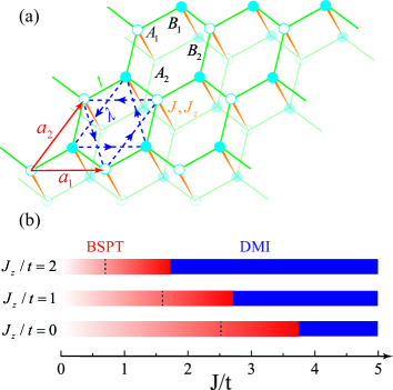
Figure 1: (Color online) (a) Illustration of AA-stacked honeycomb ribbon ($L_{\mathbf{a}_{1}}=3$, $L_{\mathbf{a}_{2}}=3$) with periodic (open) boundary condition along the $\mathbf{a}_{1}$ ($\mathbf{a}_{2}$) direction. $\mathbf{a}_{1}=(1,0)$ and $\mathbf{a}_{2}=(1/2,\sqrt{3}/2)$ are the primitive translation vectors. $A_{1}$, $B_{1}$, $A_{2}$ and $B_{2}$ are the four sublattices within one unit cell. (b) $J$-$J_{z}$ phase diagram of bilayer Kane-Mele-Hubbard model. The bosonic SPT (BSPT, red) and dimer Mott insulator (DMI, blue) phases are separated by a bulk transition. The dashed lines inside BSPT denote the $J$ values, above which one can clearly see the exponential decay of the single-particle Green’s function at the boundary from our finite-size calculations. The relative range of such region becomes wider as $J_{z}$ increases.

Recently it was proposed that instead of directly studying bosonic systems, the physics of bosonic SPT states can be mimicked by interacting fermionic systems, in the sense that its low energy physics is completely identical to bosonic SPT states You et al. (2015). For example, in an interacting fermion model on the AA-stacked bilayer Kane-Mele-Hubbard model, a bona fide interaction-driven topological phase transition has been studied in our previous papers Slagle et al. (2015); He et al. (2016a, b). A direct continuous quantum phase transition between a quantum spin Hall (QSH) phase and a topologically trivial Mott insulator was found via large-scale quantum Monte Carlo (QMC) simulations. At the critical point, only the bosonic spin and charge gaps are closed, while the bulk single-particle excitations remain open. This transition can be described by a $(2+1)d$ $O(4)$ nonlinear sigma model with a topological $\Theta$-term Xu and Ludwig (2013); Slagle et al. (2015); He et al. (2016a). However, as for the physics on the edge, although the field theory and renormalization group analysis You et al. (2016) provide us with analytical evidence of a gapless bosonic edge, which is supported by an extended version of dynamical mean-field theory calculation at finite temperaturesYoshida and Kawakami (2016), unbiased numerical evidence that can prove the conclusion is still demanded, and it is the task of this paper.

Here, we employ large-scale QMC simulation to the zigzag ribbon geometry, i.e., the bilayer Kane-Mele-Hubbard model with periodic boundary condition along the $\mathbf{a}_{1}$ direction and open boundary along the $\mathbf{a}_{2}$ direction [see Fig. 1 (a)]. On finite-size ribbon, our unbiased results unveil a substantial region ($\sim t$) of bosonic SPT phase from the exponential decay of the single-particle Green’s function along the boundary before the bulk quantum phase transition, while the gapless $O(4)$ bosonic modes prevail on the edge with power-law correlation functions.

Model and method. The Hamiltonian He et al. (2016a); You et al. (2016) of the AA-stacked bilayer Kane-Mele-Hubbard model is given by

$$\begin{split}\hat{H}&=-t\sum_{\xi\langle i,j\rangle\alpha}(\hat{c}_{\xi i\alpha}^{\dagger}\hat{c}_{\xi j\alpha}+\hat{c}_{\xi j\alpha}^{\dagger}\hat{c}_{\xi i\alpha})\\ &+i\lambda\sum_{\xi\langle\langle i,j\rangle\rangle\alpha\beta}\nu_{ij}(\hat{c}_{\xi i\alpha}^{\dagger}\sigma_{\alpha\beta}^{z}\hat{c}_{\xi j\beta}-\hat{c}_{\xi j\beta}^{\dagger}\sigma_{\beta\alpha}^{z}\hat{c}_{\xi i\alpha})\\ &-\frac{J}{8}\sum_{i}\left[(\hat{D}_{1i,2i}+\hat{D}_{1i,2i}^{\dagger})^{2}-(\hat{D}_{1i,2i}-\hat{D}_{1i,2i}^{\dagger})^{2}\right]\\ &-\frac{J_{z}}{4}\sum_{i}\left[(\hat{n}_{1i\uparrow}-\hat{n}_{1i\downarrow})-(\hat{n}_{2i\uparrow}-\hat{n}_{2i\downarrow})\right]^{2},\end{split}$$ (1)

with $\hat{D}_{1i,2i}=\sum_{\sigma}\hat{c}_{1i\sigma}^{\dagger}\hat{c}_{2i\sigma}$. Here $\alpha$, $\beta$ denote the spin species and $\xi=1,2$ stand for the layer index. The first term in Eq. (1) describes the nearest-neighbor hopping [green lines in Fig. 1 (a)] and the second term represents spin-orbital coupling $\lambda/t=0.2$ [blue lines with arrows in Fig. 1 (a)]. The third term $J$ is the interlayer antiferromagnetic Heisenberg (approximated) interaction He et al. (2016a), and the last term $J_{z}$ denotes the interlayer antiferromagnetic Ising (approximated) interaction You et al. (2016). When $J/t>0$ and $J_{z}/t>0$, we can prove that there is no fermion sign problem in the QMC calculations You et al. (2016).

This Hamiltonian possesses a high symmetry, $SO(4)\times SO(3)$ He et al. (2016a); You et al. (2016). When $J_{z}/t=0$, in the bulk, $J$ drives a continuous quantum phase transition from a QSH phase to an interlayer dimer phase at $J_{c}/t\approx 3.73$, and since there is no spontaneous symmetry breaking at both sides of this transition, it is dubbed as a bona fide interaction-driven topological phase transition He et al. (2016a). On the other hand, when $J/t=0$, it is perceivable that $J_{z}$ will eventually drive the system into a spin-density-wave phase with magnetization along the $z$ direction (SDW-Z) which spontaneously breaks the $SO(3)$ symmetry and time-reversal symmetry. Our numerical data shows that the SDW-Z order establishes when $J_{z}/t>2$. More information about the $J-J_{z}$ phase diagram is given in the Supplemental Material Sup .

The QSH phase still survives when the interlayer interactions are not sufficiently strong. However, we will show that the gapless edge modes in the interacting QSH phase are carried by bosons emerging from interacting fermionic degrees of freedom, hence the system is actually in a bosonic SPT state before the bulk phase transition [the BSPT phase in Fig. 1 (b)]. This conclusion is drawn upon the numerical observation of exponential decay of a single-particle Green’s function on the edge before the bulk quantum phase transition, while at the same time bosonic $O(4)$ correlation functions present a clear power-law decay.

The QMC method employed here is the projective auxiliary-field quantum Monte Carlo approach Assaad and Evertz (2008); Meng et al. (2010). It is a zero-temperature version of the determinantal QMC algorithm. The specific implementation of the QMC method on the model in Eq. (1) is presented in Ref. He et al. (2016a). The projection parameter is chosen at $\Theta=50/t$ and the Trotter slice $\Delta\tau=0.05/t$. Since the gapless edge modes are hallmarks of SPTs, we perform the simulation with periodic (open) boundary condition along the $\mathbf{a}_{1}$ ($\mathbf{a}_{2}$) direction [see Fig. 1 (a)]. The main results in this paper are obtained from a ribbon with $L_{\mathbf{a}_{1}}=27,L_{\mathbf{a}_{2}}=9$ which is large enough to obtain controlled representation of thermodynamic limit behaviors of the BSPT phase in Fig. 1 (b).

Figure 2: (Color online) The log-log plot of single-particle Green’s function at the boundary as a function of interlayer antiferromagnetic interaction $J/t$ when (a) $J_{z}/t=0$ and (b) $J_{z}/t=1$. In both cases, results show the exponential decay before the bulk topological phase transition $J_{c}/t$.

Edge analysis. In the noninteracting limit, the bilayer Kane-Mele model supports four fermionic edge modes: two left-moving up-spin modes and two right-moving down-spin modes from both layers, respectively. They are denoted by the boundary fermion fields $c_{\xi\alpha}$ ($\xi=1,2$, $\alpha=\uparrow,\downarrow$). Following the standard Abelian bosonization procedure, we can rewrite $c_{\xi\alpha}=\kappa_{\xi\alpha}e^{i\phi_{\xi\alpha}}/\sqrt{2\pi a}$, where $a$ is a short distance cutoff and $\kappa_{\xi\alpha}$ is the Klein factor that ensures the anticommutation of the fermion operators. As we turn on the interaction, in terms of the bosonized degrees of freedom $\phi=(\phi_{1\uparrow},\phi_{2\uparrow},\phi_{1\downarrow},\phi_{2\downarrow})$, the effective action for the interacting edge modes reads

$$\begin{split}S&=\int d\tau dx\frac{1}{4\pi}(\partial_{x}\phi^{\intercal}K\partial_{\tau}\phi+\partial_{x}\phi^{\intercal}V\partial_{x}\phi)-\lambda\cos(l_{0}^{\intercal}\phi),\\ K&=\left(\begin{smallmatrix}1&&&\\ &1&&\\ &&-1&\\ &&&-1\end{smallmatrix}\right),V=v_{0}\left(\begin{smallmatrix}1&u&-g&g\\ u&1&g&-g\\ -g&g&1&u\\ g&-g&u&1\end{smallmatrix}\right),\end{split}$$ (2)

where $g=J_{z}/(4\pi v_{0}-J_{z})$, $u=(J_{z}+J)/(4\pi v_{0}-J_{z})$ and $v_{0}$ is the bare velocity of the edge modes. $\lambda\propto J$ is the backscattering term induced by the interlayer Heisenberg interaction with the corresponding charge vector $l_{0}=(1,-1,-1,1)^{\intercal}$. The scaling dimension of $\cos(l_{0}^{\intercal}\phi)$ is

$$\Delta_{0}=\frac{2(1-u-2g)}{\sqrt{(1-u)^{2}-4g^{2}}}.$$ (3)

Without the Ising interaction $J_{z}$ (i.e. $g\to 0$), the operator $\cos(l_{0}^{\intercal}\phi)$ is marginal from the scaling dimension $\Delta_{0}=2$. Further renormalization group (RG) analysisYou et al. (2016) shows that the term $\lambda\cos(l_{0}^{\intercal}\phi)$ is marginally relevant, meaning that the fermionic edge modes of the non-interacting QSH state are unstable to the interaction $J$. As long as $J$ is turned on, the boundary fermions will be gapped out by the interaction, leaving only bosonic edge modes described by the spin $c_{1\uparrow}^{\dagger}c_{1\downarrow}-c_{2\uparrow}^{\dagger}c_{2\downarrow}$ and charge $c_{1\uparrow}c_{2\downarrow}-c_{1\downarrow}c_{2\uparrow}$ fluctuations. However, due to the marginal nature of RG flow, the boundary fermion gap could be very small for small $J$, which is hard to resolve in our finite-size numerical study. The positive $J_{z}$ interaction (i.e. $g>0$) helps to boost the RG flow by reducing the scaling dimension $\Delta_{0}$ according to Eq. (3), such that $J$ becomes relevant and the gap in the single-particle (fermionic) spectrum can be observed in numerics for smaller $J$ as well. In the following, we will show that with moderate interaction $J$, the QSH edge modes indeed become bosonic at low energy, resembling the key feature of BSPT states. The interaction $J_{z}$ will help to enhance the fermion gap and make the BSPT edge modes more prominent in a finite-size system.

Numerical results. Figures 2 (a) and (b) show the single-particle Green’s function $G_{ij}^{\sigma}=\bra{\Psi}\hat{c}_{i\sigma}^{\dagger}\hat{c}_{j\sigma}\ket{\Psi}/\braket{\Psi}{\Psi}$ along the edge as a function of $J/t$, at $J_{z}/t=0$ and $1$, respectively. $\ket{\Psi}\propto e^{-\Theta\hat{H}/2}\ket{\Psi_{T}}$ is the ground state wave function projected from a trial wave function $\ket{\Psi_{T}}$ He et al. (2016a). We see a clear exponential decay before the bulk transition at $J_{c}/t\approx 3.73$ (for $J_{z}/t=0$) and $J_{c}/t\approx 2.7$ (for $J_{z}/t=1$). The exponential decay of edge single-particle Green’s function at $J<J_{c}$ indicates that fermions are no longer gapless at the boundary between our model system and a topologically trivial one (such as vacuum).

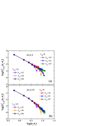
Figure 3: Illustration of finite-size effects in the single-particle Green’s function along the edge for different $L_{\mathbf{a}_{1}}$ and $L_{\mathbf{a}_{2}}$. (a) at $J/t=2.5,J_{z}/t=0$, the exponential decay of the single-particle Green’s function acquires strong finite-size effect. (b) at $J/t=2.75,J_{z}/t=0$, the finite size effect is absent and exponential decay is seen for the chosen $L_{\mathbf{a}_{1}}$ and $L_{\mathbf{a}_{2}}$.

To rule out the possible finite-size effect, we employ several different ribbon geometries in the QMC calculations. From Fig. 3 (a), it is hard to determine whether the edge single-particle Green’s function will exponentially decay in the thermodynamic limit when $J/t=2.5,J_{z}/t=0$ because of the strong finite-size effect. However, when $J/t=2.75,J_{z}/t=0$, we see a clear exponential decay no matter if $L_{\mathbf{a}_{1}}$ and $L_{\mathbf{a}_{2}}$ are even or odd, large or small, and the single-particle Green’s function has a clear trend to truly exponential decay in the thermodynamic limit.

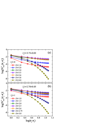
Figure 4: (Color online) The log-log plot of equal-time two-particle $O(4)$ vector correlation function at the boundary for (a) $J_{z}/t=0$ and (b) $J_{z}/t=1$. Both panels show the power-law decay behaviors before the bulk topological phase transition at $J_{c}/t$.

The exponential decay of single-particle Green’s function at the boundary in the thermodynamic limit indicates that the gapless fermion edge mode in the non-interacting case is gapped out by the interlayer exchange interaction. Hence the fermion excitations have a gap both in the bulk and on the edge He et al. (2016a). However, as shown in our edge analysis, the system can still be non-trivial in the bosonic sector You et al. (2016). To see this, we calculate the XY spin (SDW-XY) correlation function and superconducting pairing (SC) correlation function at the boundary. According to the analysis in Ref. You et al. (2016), we define them as

$$N_{AA}^{+-}(\mathbf{r}_{j}-\mathbf{r}_{i}) = \frac{1}{2}[S_{A_{1}A_{1}}^{\pm}(\mathbf{r}_{j}-\mathbf{r}_{i})-S_{A_{1}A_{2}}^{\pm}(\mathbf{r}_{j}-\mathbf{r}_{i})$$

$$- S_{A_{2}A_{1}}^{\pm}(\mathbf{r}_{j}-\mathbf{r}_{i})+S_{A_{2}A_{2}}^{\pm}(\mathbf{r}_{j}-\mathbf{r}_{i})]$$

$$\Delta_{AA}(\mathbf{r}_{j}-\mathbf{r}_{i}) = \bra{\Psi}\hat{\Delta}_{iA_{1}A_{2}}^{\dagger}\hat{\Delta}_{jA_{1}A_{2}}\ket{\Psi}/\braket{\Psi}{\Psi}$$ (4)

where $S_{mn}^{\pm}(\mathbf{r}_{j}-\mathbf{r}_{i})=\bra{\Psi}\frac{1}{2}(\hat{S}_{i}^{+}\hat{S}_{j}^{-}+\hat{S}_{i}^{-}\hat{S}_{j}^{+})\ket{\Psi}/\braket{\Psi}{\Psi}$, $m,n=A_{1},A_{2}$ denote the $A$ sublattice sites in the first and second layer. $i$ and $j$ label the unit cells. $\hat{S}^{+}_{i}$ is the spin flip operator and $\hat{\Delta}_{iA_{1}A_{2}}^{\dagger}$ is the interlayer singlet creation operator. Figures 4 (a) and (b) show the SDW-XY correlation function at the boundary as a function of $J/t$. Before the bulk quantum phase transition, they all show the power-law decay at $J<J_{c}$. Due to the $SO(4)$ symmetry, the SDW-XY and SC correlation functions are exactly the same because they rotate into each other He et al. (2016a); You et al. (2016). So the physical bosonic boundary modes are simply the SDW-XY and SC fluctuations on the boundary.

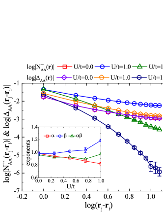
Figure 5: (Color online) Edge spin $N^{+-}_{AA}(\mathbf{r})$ and pairing $\Delta_{A_{1}A_{2}}(\mathbf{r})$ correlation functions for increasing $U/t$, at $J/t=2.75$ and $J_{z}/t=0$. The inset shows the extracted Luttinger parameters as a function of $U/t$.

Turning on an extra on-site Hubbard interaction $U\sum_{i}(\hat{n}_{i\uparrow}+\hat{n}_{i\downarrow}-1)^{2}$ (see Sec. VII in the Supplemental Material Sup for the $U/t$ path chosen in the bulk phase diagram) to our original model Eq. (1) would break the $O(4)$ symmetry, and change the scaling dimension of the spin and Cooper pair operators. According to the bosonization analysis in Ref. You et al. (2016), the spin and pairing $O(4)$ bosonic modes always have power-law correlation, with $N^{+-}_{AA}(\mathbf{r})\propto|\mathbf{r}|^{-\alpha}$ and $\Delta_{AA}(\mathbf{r})\propto|\mathbf{r}|^{-\beta}$. $\alpha$ and $\beta$ depend on the Luttinger parameters, but their product remains a universal constant: $\alpha\beta=1$. This is due to the fact that, spin and charge are a pair of conjugate variables at the boundary, which is a physical consequence of the SPT state in the bulk. This prediction is confirmed in our simulation. In Fig. 5, at $J/t=2.75$ $J_{z}/t=0$ and gradually increasing $U/t$, $N^{+-}_{AA}(\mathbf{r})$ and $\Delta_{AA}(\mathbf{r})$ have the same power law $\alpha=\beta\sim 1$ at $U/t=0$, but as $U/t$ increases, $\alpha$ and $\beta$ start to deviate, but their product $\alpha\beta$ remains close to $1$, as shown in the inset of Fig. 5, until the bulk transition to a SDW-XY phase at $U_{c}/t\sim 1.3$ He et al. (2016a); Sup .

Discussion. In this paper, we have performed QMC simulation for a proposed interacting lattice fermion model, and explicitly demonstrated that this system shows a bosonic SPT state, in the sense that the boundary has gapless bosonic modes, but no gapless fermionic modes under interaction. Recently it was also proposed that the same physics can be realized in an AB stacking bilayer graphene under a strong out-of-plane magnetic field and Coulomb interaction Bi et al. (2016). Our model, though technically different, should belong to the same topological class, and it has the advantage of being sign problem free for QMC simulation. Unbiased information of such a strongly correlated system, including transport and spectral properties, can be obtained from QMC simulation, and quantitative comparison with the up-coming experiments is hence made possible.

Supplemental material: Visualizing a Bosonic Symmetry Protected Topological Phase in an Interacting Fermion Model

I I.$J_{z}/t=2$ results

Fig. S1 shows the single-particle Green’s function and SDW-XY correlation function at the ribbon edge as a function of interlayer $J/t$ interaction when $J_{z}/t=2$. The bulk quantum critical point is obtained from energy curves and SDW-XY magnetic structure factors which will be shown in the following section. The $J_{z}/t=2$ case shares the similar behavior as the $J_{z}/t=0$ and $1$ cases. The single-particle Green’s function at the ribbon edge shows the exponential decay before the bulk quantum phase transition, while the SDW-XY correlation function still decays as a power-law behavior.

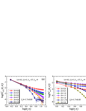
Figure S1: Single-particle Green’s function (a) and SDW-XY correlation function (b) at the ribbon edge as a function of $J/t$ when $J_{z}/t=2$.

II II. magnetic orders

The Ising-like $J_{z}$ term in our Hamiltonian can be decompose into the following three terms,

$$-\frac{J_{z}}{4}\sum_{i}\left[(\hat{n}_{1i\uparrow}-\hat{n}_{1i\downarrow})-(\hat{n}_{2i\uparrow}-\hat{n}_{2i\downarrow})\right]^{2}=-\frac{J_{z}}{4}\sum_{\xi,i,\sigma}\hat{n}_{\xi i\sigma}+\frac{J_{z}}{2}\sum_{\xi,i}\hat{n}_{\xi i\uparrow}\hat{n}_{\xi i\downarrow}+2J_{z}\sum_{i}\hat{S}_{1i}^{z}\hat{S}_{2i}^{z}$$ (S1)

The first term is the on-site potential term, the second term is the on-site Coulomb repulsive interaction and the third term is the Ising exchange interaction between two layer sites. When $J_{z}\gg J$, $J_{z}$ will drive the system into a Ising antiferromagnetic ordered (SDW-Z) state. We define the SDW-Z antiferromagnetic magnetic order along $z$ direction as follows

$$\begin{split}M_{AA}^{zz}(\mathbf{r}_{j}-\mathbf{r}_{i})=&S_{A_{1}A_{1}}^{zz}(\mathbf{r}_{j}-\mathbf{r}_{i})-S_{A_{1}A_{2}}^{zz}(\mathbf{r}_{j}-\mathbf{r}_{i})-S_{A_{2}A_{1}}^{zz}(\mathbf{r}_{j}-\mathbf{r}_{i})+S_{A_{2}A_{2}}^{zz}(\mathbf{r}_{j}-\mathbf{r}_{i})\\ S_{mn}^{zz}(\mathbf{r}_{j}-\mathbf{r}_{i})=&\bra{\Psi}\hat{S}_{i}^{z}\hat{S}_{j}^{z}\ket{\Psi}/\braket{\Psi}{\Psi},i\in m,j\in n\end{split}$$ (S2)

From Fig. S2, there is no SDW-XY and SDW-Z magnetic orders (and no time-reversal symmetry breaking) in the whole $J/t>0$ parameter regime when $J_{z}/t\leq 2.0$. However, when $J_{z}/t=3.0$, SDW-Z order emerges in the middle of $J/t$ parameter region.

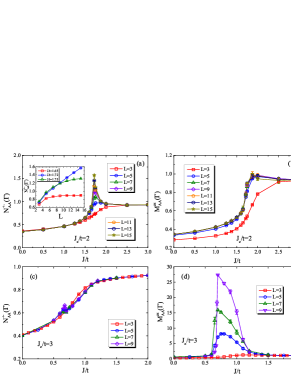
Figure S2: SDW-XY (a,c) and SDW-Z (b, d) structure factor as a function of $J/t$ and linear system size $L$ for $J_{z}/t=2$ and $J_{z}/t=3$. There is no SDW-Z magnetic order when $J_{z}/t\leq 2$ in the whole $J/t$ regime. Around the bulk quantum phase transition critical point (QCP), SDW-XY structure factor shows a power-law increasing tendency with system size $L$, however, the power-law increasing exponent is less than 2 which means no SDW-XY magnetic order will develop around the QCP in the thermodynamic limit.

III III. Energy curves

We plot the expectation values of four parts of the Hamiltonian in Fig. S3 as a function of $J/t$ for different $J_{z}/t$ values. From the inflection point of the energy curves and magnetic structure factor shown in Fig. S2, we can obtain the approximate bulk quantum phase transition points without calculating the energy gaps.

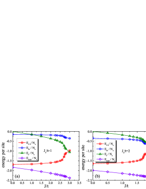
Figure S3: Ground state energy per site as a function of $J/t$ when $J_{z}/t=1$ and $2$. The linear system size used here is $L=15$. Combined with Fig. S2, we can get the phase diagram which is shown in Fig.1 (b) in the main text.

IV IV. Other matrix elements of edge Green’s function and O(4) correlation function

In the main text, we only show the Green function between $A_{1}$ sublattice and $B_{1}$ sublattice in the same layer along the ribbon edge, i.e., an off-diagonal term of the edge Green’s function matrix. Here, we present that the diagonal parts of Green function matrix also show similar behavior as the off-diagonal part.

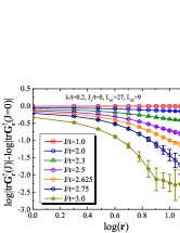
Figure S4: The trace of single-particle Green’s function matrix at the ribbon edge as a function of $J/t$ when $J_{z}/t=0$.

Fig. S4 shows the trace of single-particle Green’s function matrix $\text{Tr}\mathbf{G}_{\mathbf{r}}^{\uparrow}=G_{A_{1}A_{1}}^{\uparrow}+G_{A_{2}A_{2}}^{\uparrow}+G_{B_{1}B_{1}}^{\uparrow}+G_{B_{2}B_{2}}^{\uparrow}$ at the ribbon edge as a function of $J/t$ when $J_{z}/t=0$. The diagonal part of single-particle Green’s function at the edge also shows the exponential decay before the bulk quantum phase transition.

For the SDW-XY correlation matrix, we have show the $|N_{AA}^{+-}|$ (with combined elements) in the main text. Here, we also show you the power-law decay of $|N_{BB}^{+-}|$ and $|S_{A_{1}B_{1}}^{+-}|$ before the bulk quantum phase transition in Fig. S5, where $N_{BB}^{+-}$ defines as

$$N_{BB}^{+-}(\mathbf{r}_{j}-\mathbf{r}_{i})=\frac{1}{2}[S_{B_{1}B_{1}}^{\pm}(\mathbf{r}_{j}-\mathbf{r}_{i})-S_{B_{1}B_{2}}^{\pm}(\mathbf{r}_{j}-\mathbf{r}_{i})-S_{B_{2}B_{1}}^{\pm}(\mathbf{r}_{j}-\mathbf{r}_{i})+S_{B_{2}B_{2}}^{\pm}(\mathbf{r}_{j}-\mathbf{r}_{i})].$$ (S3)

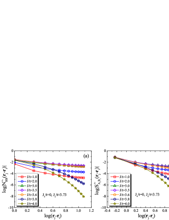
Figure S5: The SDW-XY correlation functions $|N_{BB}^{+-}|$ and $|S_{A_{1}B_{1}}^{+-}|$ at the ribbon edge as a function of $J/t$ when $J_{z}/t=0$.

V V. Finite-size effects

In the main text, we mainly use the $L_{a_{1}}=27,L_{a_{2}}=9$ system size in the PQMC calculations. Here, we show that $L_{a_{2}}=9$, which is the width of the ribbon, is large enough to obtain thermodynamic limit behavior. As shown in Fig. S6, when we increase the $L_{a_{2}}$ from 5 to 11, little change both in the single-particle Green’s function as well as two-particle bosonic correlation function, can be observed.

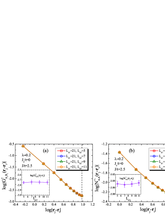
Figure S6: The single-particle Green’s function and SDW-XY correlation function at the ribbon edge change little when we increase $L_{a_{2}}$ from 5 to 11. The insets show the y-axis values of the right-most points as a function of ribbon width $L_{a_{2}}$.

VI VI. Strange Correlator

Apart from creating a physical spatial edge to study the edge physics, we can also calculate the strange correlator to reflect the physical edge between two topological distinct many-body ground state wave functions You et al. (2014); Wu et al. (2015).

$$C(r,r^{\prime})=\frac{\bra{\Omega}\hat{\phi}(r)\hat{\phi}(r^{\prime})\ket{\Psi}}{\braket{\Omega}{\Psi}}$$ (S4)

we can define the single-particle strange correlator and spin strange correlator by replacing the bra state with a topological trivial state $\bra{\Omega}$ in Eq. (4) in the main text. The single-particle strange correlator also shows an exponential decay before the bulk quantum phase transition while the spin strange correlator remains power-law decay, indicating the interacting QSH phase $\ket{\Psi}$ is topologically distinct from the trivial phase $\bra{\Omega}$, and there exist gapless bosonic modes at the spatial interface between two systems.

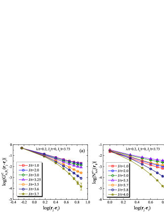
Figure S7: single-particle strange correlator and SDW-XY strange correlator as a function of $J/t$ when $J_{z}/t=0$.

VII VII. on-site $U$ interaction

The phase diagram of bilayer KMH model with on-site $U\sum_{i}(\hat{n}_{i\uparrow}+\hat{n}_{i\downarrow}-1)^{2}$ interaction and inter-layer $J$ interaction is shown in Fig. S8 (a). The phase boundaries are obtained from the bosonic gap closing as well as the nonzero magnetic order parameter in our previous paper Ref. He et al. (2016a). Based on the exponential decay of edge single-particle Green’s function in Fig. S8 (b) and the power-law decay of edge SDW-XY correlation function in Fig. 5 in the main text, we conclude that the quantum spin Hall phase with finite interaction $U$ and $J$ which is shown in Fig. S8 (a) is also a bosonic SPT phase.

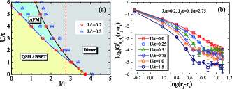
Figure S8: (a) Phase Diagram of bilayer KMH model with on-site $U$ interaction and inter-layer $J$ interaction. The red line shows the vertical phase path we used in Fig. 5 in the main text. The exponential decay of single-particle Green’s function at the ribbon edge indicates that fermions are still gapped when $U/t$ is increased at $J/t=2.75$.