Estimating the Handicap Effect in the Go Game:
A Regression Discontinuity Design Approach

Abstract

This paper provides an estimate for the handicap effect in the go game, a board game widely played in Asia and other parts of the world. The estimation utilizes a unique handicap assignment rule of the game, where the amount of handicaps changes discontinuously with the players’ strengths. A dataset suitable for this estimation strategy is collected from game archives of an online platform. The result implies that an additional handicap typically changes the game odds by about 30 percent points, while the impact varies across the handicap level.

1 Introduction

Handicapping is a practice frequently applied in competitive games and sports for the purpose of equalizing the players’ chances of winning. When the abilities of players differ so much that competition under the standard setup is considered ineffective, certain disadvantage is imposed on the more skilled player, so that the game odds become close to even. With appropriate amount of handicaps, diverse levels of contestants can participate in the same tournament, or tutoring sessions become more effective.

An effective assignment of handicaps requires reliable prediction of their impact. However, statistical inference on the handicapping impact is often challenging since it by nature suffers from selection bias; People play handicapped games because their ability gap is large. Hence players playing even games are not necessarily comparable with those playing handicapped games. Naive comparison of games with and without handicaps would produce a biased estimate since it cannot filter the effect of handicaps from that resulted from other covariates.

This paper is an attempt to overcome this challenge in the case of the go game. Go is a two-player board game that originates in ancient China. It belongs to the class of two-player zero-sum games with complete information. The game is played widely in East Asia, such as China, Korea Republic, Japan, and Taiwan, while it has been gaining popularity in other areas of the world as well.

Go is played on a board with grids. The official grid size is 19 by 19, while smaller sizes are also used occasionally. In a game, players hold either black or white stones and place them at intersections of the grids by turn (See the left panel of Figure 1). The goal of the players is to enclose a larger territory, which is defined as the number of empty intersections surrounded by stones of either color. See the right panel of Figure 1 for an example of end game configuration and territory counting.

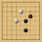
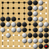
Figure 1: Left: 9 by 9 go board. Stones are placed at intersections. Right: Example of end game and territory counting. Both the black and white have 19 points. The images are generated using the software mugo (https://code.google.com/archive/p/mugo/)

In the official rule, the player who holds black makes the first move. Since he always has the same or a larger number of stones on the board than the white does, it is known that he enjoys a certain advantage throughout the game. To offset this first mover advantage, the white player is granted 6.5 (or 7.5 in Chinese rule) points at the end of the game. These additional points are called komi.

Handicapping system of the go takes advantage of the first mover advantage. If the skill levels of two players differ significantly, then the more skilled one holds white (hence becomes the second mover) without receiving komi. Hence, the black can fully enjoy the first mover advantage, which would close the skill gap to some extent. This setup is called a sen game.

If the skill gap is so large that the first mover advantage is not sufficient to fill it, the less skilled is allowed to add another stone at the beginning, typically at designated positions called stars. This setup is called a two-stone game. As the abilities are apart even further, the number of handicap stones increase to three, four and so on. See Figure 2 for opening configurations of handicapped games.

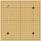
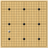
Figure 2: Left: Opening of a three stone game. Right: Opening of a nince stone game. The images are generated using the software mugo

Handicap assignment is often determined by a discrete rating called dan-kyu system. An absolute beginner is given a kyu with some large number such as 30 kyu or 30k in short. As his skill reaches certain thresholds, he gets promoted to 29k, 28k, and so on. 1k is followed by 1 dan or 1d, and the number starts to climb as 2d, 3d and so on. Typically 9d is the highest rating.

In many platforms, players with the same dan-kyu rating play even games, where their colors are determined randomly and the white player receives komi. When the ratings of the players are different, the lower ranked player is entitled as many handicaps as the rating difference. For example, 2k and 3k play sen games, where the 3k holds black with no komi given to the white. 9d and 1k, with rating difference of nine, play nine-stone games.

This assignment rule is discontinuous in players’ skill level, and hence forms a regression discontinuity design, providing a quasi-experimental situation for causal inference on the handicap effect. Suppose a 1d player plays two games, one against a “weakest” 1d, and the other against a “strongest“ 1k. While the two opponents are similar in terms of the skill levels, the setup would become even and sen respectively, due to their ratings. Thus, the difference between the two games is arguably attributable to the handicapping.

In this paper I apply this strategy to quantify the handicap effect on the game outcomes. A dataset suitable for this approach is collected from game archives of the KGS, an online go platform.

The rest of the paper is organized as follows. Section 2 describes the data. Section 3 formally states the estimation strategy. Section 4 presents the results. Section 5 concludes.

2 Data and Descriptives

2.1 Sampling players

Data for this study have been collected from the archives of the KGS, an online platform for the go game. Games played on the KGS are all stored on the server. Unless the players want otherwise, records of all rated games are open to the public. A game record is saved in a text file of the smart go format (SGF), which contains the actual move sequences and the outcome, as well as meta information such as the player IDs and ratings, and the date and time when the game started.

As far as the author recognizes, the KGS does not provide an API or quarry feature that allows for randomized sampling of the games; The games are only viewable when searched by a player ID. Hence, I first collected a list of active player IDs by manually recording the player IDs logging onto the “English game room.” For the sake of geographical heterogeneity, the sampling has been conducted at four different timings.

I also added the 100 top rated players as of May 7th, 2014 to the list. Top players on the KGS include professional players and amateurs close to that level. By including these players the findings of the analysis are more likely to be generalizable to the professionals.

The final list consists of 1940 players. Among them, 1775 players (1679 sampled and 96 top-rated) are active in a sense that they played one or more rated games in the study period. Figure 3 shows the distribution of the player ratings in dan-kyu system.

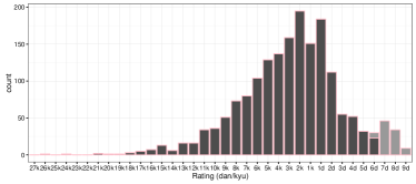
Figure 3: Distribution of the ratings in dan-kyu system. The darker bars indicates the number of sampled players, while the lighter indicates the top rated players. This chart covers 1775 players who played at least one rated game in the period between March 30, 2013 and May 13th, 2014.

2.2 Data processing

For each player, all rated games in the past four-hundred and ten days were collected (from March 30, 2013 through May 13th, 2014). Games before that was not collected because, as described below, players’ continuous rating is only available for the past four-hundred days. Hence, collecting data of older games does not increase the size of the final dataset. Each game record contains player IDs and their rating in the dan-kyu system, the date and time when the game started, the number of handicap stones and komi, and the game outcome.

The process above yields a list of player IDs, including the sampled players as well as their opponents. For each player, the image file of the rating history is downloaded from the KGS archives, which shows a time series plot of the player’s rating. The file indicates not only the discrete dan/kyu rating of the player, but also how high or low the player is rated within the same dan/kyu rating. An example of the rating graph is shown in Figure 4. The graph is updated in daily basis, and covers at longest the period since 400 days ago through the present.

The pixel information of the image files were processed to recover the time series of the players’ ratings in a continuous scale. The results are then merged with the game record data using the starting time of games as the key.

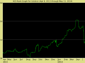
Figure 4: Example of a KGS rating plot. The rating history of the past 400 days is provided as a PNG image file. Charts are updated daily. Player ID is made blur by the author.

2.3 Data filtering

I removed the games where the continuous rating is missing for a player or both from the analysis. Missing values can occur if the ID has been deleted or inactive for a long period, and hence the rating graph is not available. I also removed the games where the rating of a player or both is unstable, indicated by a question mark added to the discrete rating (e.g. 3k?). This means that the player has not played as many games recently as the KGS system can evaluate his or her rating at a certain credible level.

Further, I removed the games with a non-standard handicap setup. At default, the lower ranked player receives as many handicap stones as the difference in the dan/kyu ratings. For example, players play even games (no handicap stone, the white receives 6.5 or 7.5 points as komi) if they have the same discrete rating. For one rank difference (e.g. 3d vs 4d, 1k vs 1d), games are played at the sen setting; The higher ranked player takes the white with only 0.5 points of komi. For larger rank differences, the lower ranked player is entitled one handicap stone per each rank deviation. For example, 1d and 3d, two rank difference, play a two-stone game, where 3d takes the white. Most of the games in the dataset follow these standard setup of the KGS. The games deviating from it are possibly arranged specifically between the players, and thus removed from the analysis.

After applying the above filtering, 85 percent of the game records remained. The final dataset has 895,050 games with 47,348 unique players.

2.4 Descriptives

Figure 5 shows the fraction of games the white wins by the handicap level. The games are grouped by the discrete ratings of the white. Consistently across the player’s levels, white players tend to win more in games with larger handicaps. That is, the white wins more in setups where he or she plays at a more disadvantageous setting.

This unintuitive pattern can be understood as a result of selection bias. Those who play even games are not comparable with those who play handicapped games since the game setup is chosen in accordance with their skill differences. Hence, direct comparison of the winning probability across the game setup does not necessarily reflect the impact resulted from the handicapping, but may reflect the skill differences among those who play different setups. In the present case, while handicaps may give advantages to the black, the impact may not be as large as it can equalize the game odds. Causal inference on the effect of handicapping requires effective control over the selection problem.

Figure 5: Fraction of games the white wins by the handicap level. The vertical axis indicates the handicap level; 0 means even, 1 means sen games, 2 or larger numbers indicate the number of handicap stones. Despite the disadvantageous setups, the white tends to win more in heavily handicapped games.

3 Regression Discontinuity Design

The regression discontinuity design (RDD) is a framework to estimate causal impact of a binary treatment variable $X$ on some outcome measurement $Y$ (Imbens and Lemieux, 2008). The RDD requires that there exists another variable $Z$, such that $X=1$ if and only if $Z\geq c$, where $c$ is a known constant. $Z$ is called a running or forcing variable for $X$. In case the treatment $X$ is not randomly assigned, the RDD provides a quasi-randomized experiment for the treatment effect. Provided that other covariates distribute continuously at $Z=c$, the cases where $Z$ is marginally above the threshold (thus $X=1$) and the cases where $Z$ is marginally below (thus $X=0$) are quite similar except that only the former receives the treatment. Therefore this comparison allows one to estimate the causal impact of the treatment $X$.

In the context of this study, handicapping corresponds to the treatment, and its causal impact on the game outcome is of interest. The running variable can be constructed by combining the ratings of two players. Let $d_{i}$ and $r_{i}$ denote the discrete and continuous rating of the player $i$, where $i=W$ (white) or $B$ (black). Without loss of generality, assume that $d_{i}$ is given by an integer defined by $d_{i}=\lceil r_{i}\rceil$, where $\lceil x\rceil$ indicates the smallest integer greater than or equal to $x$. Then, for any nonnegative integer $H$,

$$d_{W}=d_{B}+H\Longleftrightarrow H\leq d_{W}-r_{B}<H+1$$

This implies that $d_{W}-r_{B}$ is a running variable that uniquely determines the handicap level. For example, a pair of players play an even game if and only if $d_{W}=d_{B}$, or equivalently, $0\leq d_{W}-r_{B}<1$. Similarly, a necessary and sufficient condition for the sen setup is $1\leq d_{W}-r_{B}<2$, and that for two-stone game is $2\leq d_{W}-r_{B}<3$. Generally, let $H\in\{0,1,2,\dots\}$ denote the handicap level, where $H=0$ means even, $H=1$ means sen, and $H\geq 2$ indicates the number of handicap stones. Then, a necessary and sufficient condition for the setup $H$ is $H\leq d_{W}-r_{B}<H+1$.

In the estimation, the white’s winning probability is set as the outcome measurement. The causal effect of handicapping on the winning probability is estimated taking advantage of the RDD described above. That is, the difference in the winning probability below and above $d_{W}-r_{B}=H$ in interpreted as the impact of switching the handicap level from $H-1$ to $H$.

The dataset includes cases where the running variable and the handicap level are inconsistent, that is, $d_{W}-r_{B}\not\in[H,H+1)$.. This is because players’ continuous ratings are measured with error, as they are recovered from pixel information of image files. Recent theoretical studies find that the mismeasured running would nullify the standard polynomial regression estimates (Davezies and Le Barbanchon, 2014; Yanagi, 2014), and there has been no universal solution to this problem. In this paper the treatment effect is estimated by only using the observations where the running variable and the handicap level are consistent with each other. Yu (2012) studies conditions under which this approach is valid.

4 Results

Figure 6 presents the estimated winning probability of the white as a function of the running variable $d_{W}-r_{B}$. The predictive line is estimated by polynomial logistic regression of degree two, separately for each handicap level. The gray band shows the 95% confidence interval. Within the same handicap level, white’s odds are increasing in the running variable. This is because the running variable, defined by $d_{W}-r_{B}$, indicates the relative strength of the white vis-a-vis the black.

At cutoff points, the white’s winning probability drops substantially. This reflects the impact of the handicap change, that is, the disadvantage that the white incurs by playing with an additional handicap as the opposing black player falls one rank lower.

For even games, the predicted probability is about a half at the mid point of the range. As the handicap level becomes large, however, the winning probability tends to shift upward. This is consistent with the observation that the white tends to win more in handicapped games. This implies that the handicapping tends to be insufficient for games where two players’ skills are far apart, and the game odds remain skewed towards the white.

Figure 7 summarizes the estimated magnitude of handicap impact from the local linear regression at both below and above the cutoffs (Imbens and Lemieux, 2008; Lee and Lemieux, 2010). The bandwidths are selected by the criteria suggested by Imbens and Kalyanaraman (2012). The estimation is conducted using the rdd package by Dimmery (2016). The dots and segments represent the point estimate and the corresponding confidence interval of the significance level 95%.

The estimated impact of shifting from an even game to a sen game is about 25 to 30 percent point. This means, if the skill difference between a pair of players is such that one of them wins 70 percent of the games or more in the even setup, there is a good chance that removing komi realizes closer competition.

The impact is larger for the shift from sen to two-stone game, ranging about 30 to 45 percent point. Presumably advantage on the board due to the additional stone is more effective than the point advantage that realizes only at the end of the games.

Adding the third handicap stone brings smaller impact of about 20 to 30 percent point. This can be because in both two-stone and three-stone games the white can assume one corner. As the corners are considered valuable at the beginning, the two setups may not differ as much as sen and two-stone setups do.

The estimate for the impact of the fourth handicap stone is relatively unstable due to the smaller sample size, ranging 20 to 50 percent point. The impact seems about the same or slightly larger than that of the third stone.

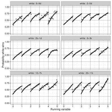
Figure 6: Predicted probability for the white to win. Each curve is estimated by polynomial logistic regression of degree two. The gray bands represent the 95% confidence intervals. The dots indicate the local averages. The drop in the probability at cutoff points can be interpreted as the correponding handicap effect.

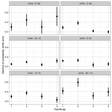
Figure 7: The handicap effect estimated by the local linear regression. Bandwidths are selected by the criteria suggested by Imbens and Kalyanaraman (2012). The dots and segments represent the point estimate and the corresponding confidence interval of the significance level 95%.

5 Concluding Remarks

This paper provides an estimate for the causal impact of handicaps in the go game, taking advantage of the regression discontinuity design due to the unique assignment rule of handicaps. Typically handicaps reduces the probability that the white wins by about 30 percent point, while variations are observed across the amount of handicaps.

Handicap assignments are often managed heuristically based on the experiences that have grown over the history. Statistical evidence as presented in this paper will help complement the practice and enhance more effective operation of games and competition.

References

- Davezies and Le Barbanchon (2014) Davezies, L. and Le Barbanchon, T. (2014). Regression Discontinuity Design with Continuous Measurement Error in the Running Variable, Working Paper 2014-27, Centre de Recherche en Economie et Statistique.
- Dimmery (2016) Dimmery, D. (2016). rdd: Regression Discontinuity Estimation. R package version 0.57.
- Imbens and Kalyanaraman (2012) Imbens, G. and Kalyanaraman, K. (2012). Optimal Bandwidth Choice for the Regression Discontinuity Estimator. Review of Economic Studies, 79 (3), 933–959.
- Imbens and Lemieux (2008) Imbens, G. W. and Lemieux, T. (2008). Regression Discontinuity Designs: A Guide to Practice. Journal of Econometrics, 142 (2), 615–635.
- Lee and Lemieux (2010) Lee, D. S. and Lemieux, T. (2010). Regression Discontinuity Designs in Economics. Journal of Economic Literature, 48 (2), 281–355.
- Yanagi (2014) Yanagi, T. (2014). The Effect of Measurement Error in the Sharp Regression Discontinuity Design, KIER Discussion Paper Series No. 910.
- Yu (2012) Yu, P. (2012). Identification of Treatment Effects in Regression Discontinuity Designs with Measurement Error.