Tensor Contractions with Extended BLAS Kernels
on CPU and GPU

Abstract

Tensor contractions constitute a key computational ingredient of numerical multi-linear algebra. However, as the order and dimension of tensors grow, the time and space complexities of tensor-based computations grow quickly. In this paper, we propose and evaluate new Blas-like primitives that are capable of performing a wide range of tensor contractions on CPU and GPU efficiently. We begin by focusing on single-index contractions involving all the possible configurations of second-order and third-order tensors. Then, we discuss extensions to more general cases.

Existing approaches for tensor contractions spend large amounts of time restructuring the data which typically involves explicit copy and transpose operations. In this work, we summarize existing approaches and present library-based approaches that avoid memory movement. Through systematic benchmarking, we demonstrate that our approach can achieve 10x speedup on a K40c GPU and 2x speedup on dual-socket Haswell-EP CPUs, using Mkl and CuBlas respectively, for small and moderate tensor sizes. This is relevant in many machine learning applications such as deep learning, where tensor sizes tend to be small, but require numerous tensor contraction operations to be performed successively. Concretely, we implement a Tucker decomposition and show that using our kernels yields atleast an order of magnitude speedup as compared to state-of-the-art libraries.

I Introduction and Scope

Multilinear algebraic computations, are ubiquitous in multiple scientific domains such as machine learning and modern data science [4], quantum chemistry and physics [14], signal and image processing [9], chemometrics [7], and biochemistry [13]. The study of tensor computations has a long and diverse history, as early as in the work by Hitchcock [11]. The domains and references provided herein are by no means exhaustive but merely a small representative sample of the various flavors in which tensor computations are used in science. Tensors are multi-way arrays which can be viewed as a generalization of matrices to allow multi-modality in data. Tensor contractions play a central role in a variety of algorithms and applications; for a motivating example, see Section II-C. However, non-trivial performance bottlenecks in several application areas are encountered due to the high space and time complexities associated with tensor computations. In this paper, motivated by the recent increased interest from machine learning and deep learning, we propose and study library-based communication avoiding approaches for performing tensor contractions.

Conventional approaches for computing general tensor contractions rely on matricization, the logical or explicit restructuring of the data so that the computation can be performed with a sequence of Basic Linear Algebra Subroutine (Blas) library calls. The Blas routines provide efficient and portable implementations of linear algebra primitives, with many fast implementations existing across many architectures [8].

To this point, the GEneral Matrix Multiply (Gemm) primitive specified within the Blas library is possibly the most optimized and widely used routine in scientific computing. Noting that the basic theoretical computational and communication complexities of most tensor contractions is equivalent to that of Gemm, these computations should scale equally well. However, we find that existing tensor libraries such as the Tensor Toolbox and Cyclops Tensor Framework perform explicit data transposition to compute almost all tensor contractions and the cost of data restructuring often dominates the cost of the actual computation. Other approaches have previously proposed intrusive compiler and static analysis solutions, whereas we provide a much simpler library-based solution [16, 17].

Findings and contributions

We introduce a new Blas primitive, known as StridedBatchedGemm, that allows the majority of tensor contractions to be computed without any explicit memory motion. We detail the so-called exceptional cases that cannot be evaluated with StridedBatchedGemm and demonstrate that an efficient solution exists with another small extension to the primitive.

We demonstrate performance improvement using our approach on both CPU and GPU in direct benchmarks in addition to an application study. The Tucker decomposition is an important tensor application in machine learning wherein the advantage of our strategy compared to existing libraries is clear.

Finally, the value of this approach and its applications are being recognized by NVIDIA. As of this writing, the proposed interface exists in the CuBlas 8.0 Release Candidate and is likely to appear the official release later this summer.

II Background

II-A Related Work

Peise et al [22] extended results from Napoli et al [19] in mapping tensor contractions to sequences of Blas routines and modeling the performance of these mappings. In this work, they systematically enumerate and benchmark combinations of possible Blas kernels one could use to compute a given tensor contraction to conclude that the best performing algorithms involve the Gemm kernel. Some evaluation strategies are neglected to be considered, such as flattening or developing new, generic linear algebraic subroutines that could yield improved performance.

Li et al [16] also recognizes the cost of explicit copies and proposes evaluation strategies exactly comparable to the flattening and batching strategies addressed in this paper. Their discussion of loop modes and component modes map to our discussion of batch modes and Gemm modes. However, Li et al do not discuss strategies beyond tensor-times-matrix multiply. Furthermore, they only consider mode-$n$ tensor-times-matrix contractions of the form $Y_{i_{1}\cdots i_{n-1}j\cdots i_{N}}=\sum_{i_{n}}X_{i_{1}\cdots i_{N}}U_{ji_{n}}$, which avoids the more complicated cases in this paper. Abdelfattah et al [3] presents a framework using batched Gemm for tensor contractions on GPUs. However, they focus on optimizing only limited number of tensor contraction kernels on extreme small size tensors. Other works in [1] [20] improve the tensor computation performance by doing loop reorganization and fusion.

The StridedBatchedGemm interface proposed in this paper has previously been mentioned by Jhurani et al [12] as a low-overhead interface for multiple small matrices on NVIDIA GPUs. Jhurani proposes the same interface for CuBlas that we propose in this paper and focuses on implementation concerns. In this work, we treat StridedBatchedGemm as an available primitive, benchmark evaluation strategies that utilize it, and examine how it may be further extended for use in multi-linear algebra.

The Blas-like Library Instantiation Software (Blis) framework [26] offers Gemms which support non-unit strides in both the row and column dimensions, which are attractive solutions to some of the problems in this paper. However, performance is expected to suffer due to decreases in cache line utilization, and SIMD opportunities.

Recent improvements in parallel and distributed computing systems have made complex tensor computation feasible. TensorFlow [2] can handle multi-linear algebra operations and it is primarily a data-flow and task-scheduling framework for machine learning.

II-B Notation

We denote tensors by uppercase letters, indices by lowercase letters and index lists by calligraphic letters. We assume all indexing is zero-based. $\mathbb{R}$ denotes the set of real numbers.

The order of a tensor is the number of modes it admits. A scalar is a zeroth-order tensor, a vector is a first-order tensor, a matrix (say $A_{mn}$) is a second-order tensor with the rows (indexed by $m$) being the first mode and columns (indexed by $n$) being the second mode, and a three-way array (say $A_{mnp}$) is a third-order tensor with the first, second and third modes indexed by $m$, $n$, and $p$, respectively. Note that we use the term index to name a mode and iterate through the elements in that mode.

The dimension of the $i^{\text{th}}$ mode, denoted dim<$i$>, is the number of elements it contains. The dimension of a mode of a tensor is denoted by the bold lowercase letter of the respective index; for example, the third-order tensor $A_{mnp}$ has dimension dim<$0$>$\times$dim<$1$>$\times$dim<$2$> or $\mathbf{m}\times\mathbf{n}\times\mathbf{p}$ where the first mode (indexed by $m$) takes values $0,\ldots,\mathbf{m}-1$, the second mode (indexed by $n$) takes values $0,\ldots,\mathbf{n}-1$, the third mode (indexed by $p$) takes values $0,\ldots,\mathbf{p}-1$.

We follow Einstein summation convention to represent tensor contractions.A general tensor contraction is written as

$$C_{\mathcal{C}}=\alpha\,A_{\mathcal{A}}\,B_{\mathcal{B}}+\beta\,C_{\mathcal{C}}$$ (1)

where $\mathcal{A},\mathcal{B},\mathcal{C}$ are ordered sequences of indices such that $\mathcal{C}\equiv(\mathcal{A}\cup\mathcal{B})\setminus(\mathcal{A}\cap\mathcal{B})$. The indices in $\mathcal{A}\cap\mathcal{B}$ are called contracted indices. The indices in $\mathcal{C}$ are called free indices.

II-C An Important Practical Application

In unsupervised learning, tensor decomposition [4] is gaining a lot of attention and is the crux of model estimation via the method of moments. A variety of problems such as topic model estimation, Gaussian mixtures model estimation, and social network learning can be provably, consistently and efficiently solved via the tensor decomposition techniques under certain mild assumptions.

The basic building blocks of these algorithms involve tensor contractions. Two frequently used tensor decomposition methods are the CP decomposition [10] and the Tucker decomposition [25]. In [27], the authors use the Tucker decomposition to extract new representations of the face images despite different expressions or camera viewpoints. To illustrate the fundamental importance of tensor contractions, we will pick one of the most common tensor decomposition algorithms, namely the higher-order orthogonal iteration (HOOI) [15] for asymmetric Tucker decomposition, and use it as a case-study. In the Einstein notation, the factorization of a third-order tensor $T\in\mathbb{R}^{\mathbf{m}\times\mathbf{n}\times\mathbf{p}}$ is given by $T_{mnp}=G_{ijk}A_{mi}B_{nj}C_{pk}$, where $G\in\mathbb{R}^{\mathbf{i}\times\mathbf{j}\times\mathbf{k}}$ is the core tensor, $A\in\mathbb{R}^{\mathbf{m}\times\mathbf{i}}$, $B\in\mathbb{R}^{\mathbf{n}\times\mathbf{j}}$, $C\in\mathbb{R}^{\mathbf{p}\times\mathbf{k}}$. From Kolda et al [24], we summarize the algorithm for the third-order tensor case in Algorithm 1. Following their notation, $T_{(r)}$ denotes the mode-$r$ unfolding of tensor $T$. For further technical details, we refer the reader to Kolda et al [24].

0:  Tensor $T\in\mathbb{R}^{\mathbf{m}\times\mathbf{n}\times\mathbf{p}}$, core tensor size $\mathbf{i}$, $\mathbf{j}$, $\mathbf{k}$, number of iterations $\mathcal{T}$.

0:  Factors $A^{\mathcal{T}}$, $B^{\mathcal{T}}$, $C^{\mathcal{T}}$ and core tensor $G$  

1:  Set $t=0$;

2:  Initialize $A^{0}\leftarrow\mathbf{i}$ leading left singular vector of $T_{(1)}$           $B^{0}\leftarrow\mathbf{j}$ leading left singular vector of $T_{(2)}$          $C^{0}\leftarrow\mathbf{k}$ leading left singular vector of $T_{(3)}$

3:  while $t<\mathcal{T}$ do

4:     $Y_{mjk}=T_{mnp}B_{nj}^{t}C^{t}_{pk}$

5:     $A^{t+1}$ $\leftarrow$ $\mathbf{i}$ leading left singular vector of $Y_{(1)}$.

6:     $Y_{ink}=T_{mnp}A^{t+1}_{mi}C^{t}_{pk}$

7:     $B^{t+1}$ $\leftarrow$ $\mathbf{j}$ leading left singular vector of $Y_{(2)}$.

8:     $Y_{ijp}=T_{mnp}B^{t+1}_{nj}A^{t+1}_{mi}$

9:     $C^{t+1}$ $\leftarrow$ $\mathbf{k}$ leading left singular vector of $Y_{(3)}$.

10:  end while

11:  $G_{ijk}=T_{mnp}A^{\mathcal{T}}_{mi}B^{\mathcal{T}}_{nj}C^{\mathcal{T}}_{pk}$

Algorithm 1 Tucker decomposition algorithm.

II-D Conventional Tensor Contraction

The conventional approach for tensor contraction is to matricize the tensors via transpositions and copies. Libraries such as Basic Tensor Algebra Subroutines (Btas) [18], MATLAB Tensor Toolbox [6, 5], and Cyclops Tensor Framework [23] all perform some version of matricization, which is typically performed in four steps:

1. Consider a general tensor contraction of the form (1). Define the index sets $\mathcal{K}$, $\mathcal{I}$, $\mathcal{J}$ as

   $$\mathcal{K}=\mathcal{A}\cap\mathcal{B},\quad\mathcal{I}=\mathcal{A}\setminus(\mathcal{A}\cap\mathcal{B}),\quad\mathcal{J}=\mathcal{B}\setminus(\mathcal{A}\cap\mathcal{B})$$

2. Permute tensors $A$, $B$, and $C$ into the form

   $$C_{\mathcal{I}\mathcal{J}}=\alpha\,A_{\mathcal{I}\mathcal{K}}\,B_{\mathcal{K}\mathcal{J}}+\beta\,C_{\mathcal{I}\mathcal{J}}$$ (2)

3. Evaluate (2) using one of four BLAS kernels:

   $$\begin{cases}\textsc{Dot}&\left|{\mathcal{K}}\right|=\left|{\mathcal{A}}\right|\text{ and }\left|{\mathcal{K}}\right|=\left|{\mathcal{B}}\right|\\ \textsc{Ger}&\left|{\mathcal{K}}\right|=0\\ \textsc{Gemv}&\left|{\mathcal{K}}\right|=\left|{\mathcal{A}}\right|\text{ xor }\left|{\mathcal{K}}\right|=\left|{\mathcal{B}}\right|\\ \textsc{Gemm}&\text{else}\end{cases}$$

4. Permute the result, $C_{\mathcal{I}\mathcal{J}}$, into the desired output, $C_{\mathcal{C}}$.

This approach to tensor contractions is completely general – it works for any two tensors of arbitrary order and any number of contraction indices. However, for even the simplest contractions, the cost of explicitly permuting the tensor data typically outweigh the cost of the computation to be performed. See Section III-A for examples.

III Approach

In this section, we present library-based evaluation strategies for performing general tensor contractions in-place – without explicit copies and/or transpositions.

III-A Motivating Observations

Figure 1: The fraction of time spent in copies/transpositions when computing the contraction $C_{mnp}=A_{mk}B_{pkn}$ using the conventional approach. Lines are shown with 1, 2, 3, and 6 total transpositions performed on either the input or output. (Left) CPU. (Right) GPU.

Case study 1

Consider $C_{mnp}=A_{mk}B_{nkp}$. The conventional approach presented in Section II-D results in an evaluation wherein one switches, by means of explicit copy operations, modes $n$ and $k$ in $B$ to produce $C_{mnp}=A_{mk}B_{knp}$, which is now of the form (2) and can be evaluated directly with a Gemm. Alternatively, we observe that we may perform the computation without explicit copy by launching $\mathbf{p}$ individual Gemms.

Case study 2

Consider $C_{mnp}=A_{km}B_{pkn}$. The conventional approach presented in Section II-D results in an evaluation wherein we may require more than one transposition. For concreteness, we analyzed how Btas performs this contraction. We observed that Btas uses four explicit transpositions that results in the following algorithm:

1. Permute $A_{km}$ to $A_{mk}$.

2. Permute $B_{pkn}$ to $B_{kpn}$.

3. Permute $C_{mnp}$ to $C_{mpn}$.

4. Compute $C_{mpn}=\alpha A_{mk}B_{kpn}+\beta C_{mpn}$ with Gemm.

5. Permute $C_{mpn}$ to $C_{mnp}$.

Similarly, in the MATLAB Tensor Toolbox, the main idea is to reshape all tensors to matrices. For instance, in Case 2.4 in Table II, it reshapes $A_{km}$ to $A_{mk}$ and reshapes tensor $B_{pkn}$ to matrix $B_{k(pn)}$ with the first dimension as $\mathbf{k}$ and the second dimension as $\mathbf{p*n}$. Cyclops also uses index reordering methods for fully dense tensors. The reordering is avoided only in the more restrictive case of high-dimensional symmetric tensors.

We note that some of the steps in the above approach can certainly be avoided with an improved algorithm that still implements the conventional approach. For example, Step 1 can be avoided by using a Gemm that implicitly transposes the first matrix via a CblasTrans parameter or equivalent in Step 4. Another optimization would be to avoid Step 3 altogether when $\beta=0$. Other approaches require even fewer transposition steps. Ultimately, observe that we may perform the computation without explicit copy by performing $\mathbf{p}$ individual Gemms.

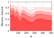
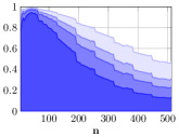
In Figure 1, we measure the cost of these explicit transpose operations in a representative tensor contraction on CPU and GPU. On the CPU we use Mkl’s mkl_somatcopy and cblas_sgemm, and on the GPU we use CuBlas’s cublasSgeam and cublasSgemm to perform each required matrix transposition and Gemm respectively. Note that transposition primitives are not specified in Blas, but are vendor-specific Blas-like extensions provided to perform common transpose operations. For this reason, these optimized functions are not typically used in tensor libraries with, instead, custom transposition implementations taking their place. These custom implementations are likely not as optimized as the vendor implementations.

As we can see from Figure 1, on the CPU, almost 40% of the time is used in copy and transpose, even when only a single mode transposition is performed. Clearly, with more transpose operations, the fraction is higher, requiring 60-80% of the total time. This correlates well with data presented in [16] where it is reported that Tensor Toolbox takes approximately 70% of the total time performing copies and transpositions in one algorithm. By avoiding these transpositions we may obtain 10x speedup on the GPU for small tensors with $\mathbf{n}\lesssim 100$, and more than 2x speedup on the CPU for almost all $\mathbf{n}$.

Although the fraction of time spent in transposition will asymptotically approach zero as $\mathbf{n}$ grows in both cases, the high bandwidth of the GPU allows the computation to dominate the communication much more quickly. Indeed, the reported maximum bandwidth of the K40c GPU is 288GB/sec and the dual-socket Xeon E5-2630 v3 CPU achieves 118GB/sec.

Additionally, that the gap between computational performance and communication performance continues to increase, so the cost of transposition is likely to increase in the future. Even now, especially for small tensor sizes, it is clear that the cost of performing explicit copies and transpositions is significant and should be avoided.

III-B Extended Notation

We would like to express evaluation strategies for tensor contractions succinctly, so we introduce additional notation.

In this paper, tensors are assumed to be stored in the column-major format. In other words, the $i^{\text{th}}$ mode has a memory stride – termed “leading dimension” in Blas – denoted ld<$i$> with $\text{\tt ld<$0$>}=1$. Using this notation, $A_{mnp}$ is stored as $A[m+n*\text{\tt ld<$1$>}+p*\text{\tt ld<$2$>}]$. Note that the common packed-storage case is obtained when, for all $i$, we have $\text{\tt ld<$i$>}=\prod_{0\leq k<i}\text{\tt dim<$k$>}$.

We now formalize three operations that are used in tensor contraction evaluations.

1. Batching: $[i]$ denotes that mode $i$ is batched, A batched mode is considered fixed.

2. Flattening: $(ij)$ denotes that modes $i$ and $j$ are flattened, i.e., modes $i$ and $j$ are now considered together as a single mode. The combined mode $h=(ij)$ is considered free.

3. Transpose: $A_{mn}^{\top}$ denotes a matrix transpose. Transposes may only be applied to tensors with exactly two free modes.

The purpose of these notations is that they map directly to looped Blas calls and the appropriate evaluation can often be read directly from the notated expression. Next, we review some rules that the above notation must follow in order to obtain a well-formed evaluation expression.

1. A batched mode $[i]$ cannot be the first mode of any matrix term. That is, $A_{[m]nk}$ is not allowed. Batching in the first mode would cause the $\mathbf{m}$ resulting logical $\mathbf{n}\times\mathbf{k}$ matrices to be strided in both rows and columns and, therefore, cannot be used as a matrix in any Blas routine.

2. A flattening $(ij)$ requires that ld<$j$> = ld<$i$> dim<$i$>. Unfortunately, the notation alone is therefore not sufficient to determine which modes may be flattened; it is contingent on the representation as well. In the common packed-storage case, however, this flattening condition is always true.

3. If a flattening operation occurs on the right side, it must occur on the left side with the same modes in the same order. For example, $C_{m(np)}$ = $A_{mk}B_{k(pn)}$ is not allowed.

4. Standard transposition rules apply: $C_{nm}^{\top}$ = $A_{mk}B_{kn}$ implies $C_{nm}$ = $B_{kn}^{\top}A_{mk}^{\top}$. However, modes may not be swapped under transposition. For example, $A_{mk}^{\top}$ can not be replaced with $A_{km}$.

This notation allows us to quickly read off the intended extended Blas evaluation expression for arbitrary tensor contractions. See Table I for examples.

Contraction	Blas Evaluation
$C_{m(np)}=A_{mk}B_{k(np)}$		Gemm (’N’,’N’, $\mathbf{m}$, $\mathbf{np}$, $\mathbf{k}$, 1, $A$, lda<1>, $B$, ldb<1>, 0, $C$, ldc<1>);
$C_{(mn)p}=B_{(mn)k}A_{pk}^{\top}$		Gemm (’N’,’T’, $\mathbf{mn}$, $\mathbf{p}$, $\mathbf{k}$, 1, $B$, $\texttt{ldb<1>}\cdot\texttt{ldb<2>}$, $A$, lda<1>, 0, $C$, $\texttt{ldc<1>}\cdot\texttt{ldc<2>}$);
$C_{m[n]p}=A_{mk}B_{k[n]p}$	for $n$ in [0,$\mathbf{n}$)	Gemm (’N’,’N’, $\mathbf{m}$, $\mathbf{p}$, $\mathbf{k}$, 1, $A$, lda<1>, $B+n\cdot\texttt{ldb<1>}$, ldb<2>, 0, $C+n\cdot\texttt{ldc<1>}$, ldc<2>);
$C_{mn[p]}=B_{k[p]m}^{\top}A_{kn}$	for $p$ in [0,$\mathbf{p}$)	Gemm (’T’,’N’, $\mathbf{m}$, $\mathbf{n}$, $\mathbf{k}$, 1, $B+p\cdot\texttt{ldb<1>}$, ldb<2>, $A$, lda<1>, 0, $C+p\cdot\texttt{ldc<2>}$, ldc<1>);
$C_{[n]p}=B_{pk}A_{k[n]}$	for $n$ in [0,$\mathbf{n}$)	Gemv (’N’, $\mathbf{p}$, $\mathbf{k}$, 1, $B$, ldb<1>, $A+n\cdot\texttt{lda<1>}$, 1, 0, $C+n$, ldc<1>);

TABLE I: Example mapping between tensor contractions with batched and flattened modes in our notation and the corresponding Blas expression evaluation. Note that the appropriate Blas primitive, transposition, matrix pointer, and leading dimension parameters to Gemm can be read off directly from the notation.

III-C BatchedGemm

Figure 2: The arithmetic intensity of computing $\mathbf{n}$ Gemms of size $\mathbf{n}\times\mathbf{n}$ versus the achieved performance on a K40c GPU and 16 cores (32 threads) of a dual socket CPU.

Instead of relying on explicit mode transpositions, Peise et al [21, 22] considered mapping tensor contractions to Blas primitives directly – enumerating all possible Blas primitives that could be used and their nesting within loops. Of course, the evaluation strategies that relied on level-3 Blas primitives (Gemm) rather than level-2 primitives (Gemv, Ger) were much more efficient. This often resulted in the need for many small Gemms to be performed, which usually does not achieve ideal performance.

The need to compute many small Gemms has not gone unnoticed by the leading implementations of Blas. NVIDIA supplied the capability to multiply pairs of many small matrices in CuBlas v4.1 [CUDA Toolkit v4.1] via the function cublasXgemmBatched. Similarly, as of Mkl 11.3$\beta$, cblas_Xgemm_batch is available with a similar interface and is also specifically optimized for small matrix sizes.

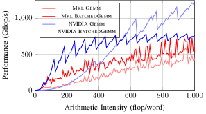
In Figure 2, we plot the achieved performance on CPU and GPU of these BatchedGemm functions by evaluating $\mathbf{n}$ Gemms of size $\mathbf{n}\times\mathbf{n}$ using each strategy with Mkl 11.3.1 and CuBlas 7.5. Note that there are much higher performance in both cases when $\mathbf{n}$ is small. When $\mathbf{n}$ is large, there is clearly room for optimization in cublasSgemmBatched.

Both of these interfaces are based on pointers to matrix pointers, which often require allocation and/or precomputation at the point-of-call. This makes them awkward to use in the context of tensor contractions where the strides between matrices are regular and the generality provided by these interfaces goes unused.

III-D StridedBatchedGemm

Building on the BatchedGemm extensions to Blas, we propose StridedBatchedGemm (Listing 1) which offers a simplified interface for the constant-strided BatchedGemm and more optimizations opportunities for implementors. The interface and reference implementation of StridedBatchedGemm is provided in Listing 1. The lda, ldb, ldc parameters are the standard “leading dimension” parameters that appear in level-3 Blas primitives and denote to the stride between columns of the matrix. We refer to the new loa, lob, loc parameters as the “leading order” parameters and denote the stride between matrices of the batch.

There are a number of advantages to a StridedBatchedGemm primitive. First, StridedBatchedGemm is actually more restrictive than the BatchedGemm that has already appeared in Mkl and CuBlas, but we argue that a BatchedGemm with a constant stride between matrices is a common enough case to consider specializing for. By providing this interface, the common case with constant strides between matrices is not forced to perform allocations or precomputations as it currently must perform in order to use BatchedGemm. Additionally, these extra restrictions provide additional knowledge of the memory layout of the computation and offers additional optimizations opportunities in SIMDization, prefetching, and tiling. In other words, the ”batch-loop” in StridedBatchedGemm now directly participates in the polyhedral computation as an affine for-loop. With the pointer-interface in BatchedGemm, the ”batch-loop” cannot fully participate in a polyhedral model of the computation and is certainly not a candidate for vectorization or cache blocking.

Case	Contraction	Kernel1	Kernel2	Kernel3	Case	Contraction	Kernel1	Kernel2
1.1	$A_{mk}B_{knp}$	$C_{m(np)}=A_{mk}B_{k(np)}$	$C_{mn[p]}=A_{mk}B_{kn[p]}$	$C_{m[n]p}=A_{mk}B_{k[n]p}$	4.1	$A_{kn}B_{kmp}$	$C_{mn[p]}=B_{km[p]}^{\top}A_{kn}$
1.2	$A_{mk}B_{kpn}$	$C_{mn[p]}=A_{mk}B_{k[p]n}$	$C_{m[n]p}=A_{mk}B_{kp[n]}$		4.2	$A_{kn}B_{kpm}$	$C_{mn[p]}=B_{k[p]m}^{\top}A_{kn}$
1.3	$A_{mk}B_{nkp}$	$C_{mn[p]}=A_{mk}B_{nk[p]}^{\top}$			4.3	$A_{kn}B_{mkp}$	$C_{mn[p]}=B_{mk[p]}A_{kn}$
1.4	$A_{mk}B_{pkn}$	$C_{m[n]p}=A_{mk}B_{pk[n]}^{\top}$			4.4	$A_{kn}B_{pkm}$	$TRANS(A_{kn}^{\top}B_{pk[m]}^{\top})$	$C_{[m][n]p}=B_{pk[m]}A_{k[n]}$
1.5	$A_{mk}B_{npk}$	$C_{m(np)}=A_{mk}B_{(np)k}^{\top}$	$C_{mn[p]}=A_{mk}B_{n[p]k}^{\top}$		4.5	$A_{kn}B_{mpk}$	$C_{mn[p]}=B_{m[p]k}A_{kn}$
1.6	$A_{mk}B_{pnk}$	$C_{m[n]p}=A_{mk}B_{p[n]k}^{\top}$			4.6	$A_{kn}B_{pmk}$	$TRANS(A_{kn}^{\top}B_{p[m]k}^{\top})$	$C_{[m][n]p}=B_{p[m]k}A_{k[n]}$
2.1	$A_{km}B_{knp}$	$C_{m(np)}=A_{km}^{\top}B_{k(np)}$	$C_{mn[p]}=A_{km}^{\top}B_{kn[p]}$	$C_{m[n]p}=A_{km}^{\top}B_{k[n]p}$	5.1	$A_{pk}B_{kmn}$	$C_{(mn)p}=B_{k(mn)}^{\top}A_{pk}^{\top}$	$C_{m[n]p}=B_{km[n]}^{\top}A_{pk}^{\top}$
2.2	$A_{km}B_{kpn}$	$C_{mn[p]}=A_{km}^{\top}B_{k[p]n}$	$C_{m[n]p}=A_{km}^{\top}B_{kp[n]}$		5.2	$A_{pk}B_{knm}$	$C_{m[n]p}=B_{k[n]m}^{\top}A_{pk}^{\top}$
2.3	$A_{km}B_{nkp}$	$C_{mn[p]}=A_{km}^{\top}B_{nk[p]}^{\top}$			5.3	$A_{pk}B_{mkn}$	$C_{m[n]p}=B_{mk[n]}A_{pk}^{\top}$
2.4	$A_{km}B_{pkn}$	$C_{m[n]p}=A_{km}^{\top}B_{pk[n]}^{\top}$			5.4	$A_{pk}B_{nkm}$	$TRANS(B_{nk[m]}A_{pk}^{\top})$	$C_{[m]n[p]}=B_{nk[m]}A_{[p]k}$
2.5	$A_{km}B_{npk}$	$C_{m(np)}=A_{km}^{\top}B_{(np)k}^{\top}$	$C_{mn[p]}=A_{km}^{\top}B_{n[p]k}^{\top}$		5.5	$A_{pk}B_{mnk}$	$C_{(mn)p}=B_{(mn)k}A_{pk}^{\top}$	$C_{m[n]p}=B_{m[n]k}A_{pk}^{\top}$
2.6	$A_{km}B_{pnk}$	$C_{m[n]p}=A_{km}^{\top}B_{p[n]k}^{\top}$			5.6	$A_{pk}B_{nmk}$	$TRANS(B_{n[m]k}A_{pk}^{\top})$	$C_{[m]n[p]}=B_{n[m]k}A_{[p]k}$
3.1	$A_{nk}B_{kmp}$	$C_{mn[p]}=B_{km[p]}^{\top}A_{nk}^{\top}$			6.1	$A_{kp}B_{kmn}$	$C_{(mn)p}=B_{k(mn)}^{\top}A_{kp}$	$C_{m[n]p}=B_{km[n]}^{\top}A_{kp}$
3.2	$A_{nk}B_{kpm}$	$C_{mn[p]}=B_{k[p]m}^{\top}A_{nk}^{\top}$			6.2	$A_{kp}B_{knm}$	$C_{m[n]p}=B_{k[n]m}^{\top}A_{kp}$
3.3	$A_{nk}B_{mkp}$	$C_{mn[p]}=B_{mk[p]}A_{nk}^{\top}$			6.3	$A_{kp}B_{mkn}$	$C_{m[n]p}=B_{mk[n]}A_{kp}$
3.4	$A_{nk}B_{pkm}$	$TRANS(A_{nk}B_{pk[m]}^{\top})$	$C_{[m][n]p}=B_{pk[m]}A_{[n]k}$		6.4	$A_{kp}B_{nkm}$	$TRANS(B_{nk[m]}A_{kp})$	$C_{[m]n[p]}=B_{nk[m]}A_{k[p]}$
3.5	$A_{nk}B_{mpk}$	$C_{mn[p]}=B_{m[p]k}A_{nk}^{\top}$			6.5	$A_{kp}B_{mnk}$	$C_{(mn)p}=B_{(mn)k}A_{kp}$	$C_{m[n]p}=B_{m[n]k}A_{kp}$
3.6	$A_{nk}B_{pmk}$	$TRANS(A_{nk}B_{p[m]k}^{\top})$	$C_{[m][n]p}=B_{p[m]k}A_{[n]k}$		6.6	$A_{kp}B_{nmk}$	$TRANS(B_{n[m]k}A_{kp})$	$C_{[m]n[p]}=B_{n[m]k}A_{k[p]}$

TABLE II: List of 36 possible single mode contraction operations between a second-order tensor and a third-order tensor and possible mappings to Level-3 Blas routines. Note that 8 cases may be performed with Gemm, 28 cases may be performed with StridedBatchedGemm, and 8 cases remain exceptional.

In Table II, we have enumerated all unique single-mode contractions between a second-order and third-order tensor using the notation from Section III-B. All but 8 contractions can be computed with only a single call to StridedBatchedGemm.

III-E Exceptional Cases

The eight exceptional cases in Table II – Cases 3.4, 3.6, 4.4, 4.6, 5.4, 5.6, 6.4, and 6.6 – occur when batching forces the evaluation to either be a BatchedGemv or violate the no-first-mode rule.

This can be resolved by making an extension to the operation parameters allowed for BatchedGemm. Typically, the available operation parameters are “normal”, “transpose”, “conjugate”, and “Hermitian”. To account for the exceptional cases, “extended X” could be added to allow violations of the no-first-mode rule and consider all three modes involved in the batching simultaneously.

For example, Case 3.6 and 6.4 could then be written

$$C_{mn[p]}=B_{[p]mk}\,A_{nk}^{\top} C_{m[n]p}=B_{[n]km}^{\top}\,A_{kp}$$

and evaluated via

sb_gemm(OP_EX_N, OP_T,
        M, N, K,
        1,
        B, ldb<1>, ldb<2>,
        A, lda<1>, 0,
        0,
        C, ldc<1>, ldc<2>,
        P);

sb_gemm(OP_EX_T, OP_N,
        M, P, K,
        1,
        B, ldb<1>, ldb<2>,
        A, lda<1>, 0,
        0,
        C, ldc<2>, ldc<1>,
        N);

When the extended operation is passed, it is known that batching is in the first mode of the input which always has leading dimension 1. Thus, the leading order parameter to sb_gemm contains no information. Instead, leading dimensions of the other two modes in row-column order of the batched matrix are passed as the leading dimension and leading order parameters.

The implementation of a computation like this is expected to perform a “3D” tiling of $B$ into cache in order to efficiently contract with the standard 2D cache tiling of $A$.

III-F Generalization

In this section, we explain the generality of our approach and how it can be easily applied and extended to single-mode contractions involving tensors of arbitrary order.

Consider an arbitrary single-mode tensor contraction of the form (1). It is straightforward to see by simple counting that the number of unique contractions is $[(|\mathcal{A}|+|\mathcal{B}|-2)!]\cdot|\mathcal{A}|\cdot|\mathcal{B}|$. We note that Table II is obtained with $|\mathcal{A}|=2$ and $|\mathcal{B}|=3$. Of these contractions, all of them may be performed without explicit mode transpositions by nesting the BatchedGemm operations.

We observe that some single-mode contractions of two tensors of arbitrary order can be evaluated by batching on different modes with the BatchedGemm operations. For example, consider $C_{mn[p][q]}=A_{mk[p]}B_{nk[q]}$ wherein we can batch in either $p$ and $q$. We prefer to choose the mode with the larger dimension for the BatchedGemm batching loop over the other (nested batching).

The nested-batching strategy in Listing 2 is general and extends to any two tensors of any order. Algorithms and heuristics for choosing the looped, batched, and Gemm-ed modes are provided in Section IV-D.

Listing 1: Interface and reference implementation of BLAS-like strided batched Gemm.

⬇

// C_p = alpha*opA(A_p)*opB(B_p) + beta*C_p

sb_gemm(op_type opA, op_type opB,

int m, int n, int k,

T alpha,

const T* A, int lda, int loa,

const T* B, int ldb, int lob,

T beta,

T* C, int ldc, int loc,

int batch_size)

{

// EXPOSITION ONLY

for (int p = 0; p < batch_size; ++p)

gemm(opA, opB,

m, n, k,

alpha,

A + p*loa, lda,

B + p*lob, ldb,

beta,

C + p*loc, ldc);

}

Listing 2: Nested batching.

⬇

for (int q = 0; q < Q; ++q)

sb_gemm(OP_N, OP_T,

M, N, K,

1,

A, lda<1>, lda<2>,

B+q*ldb<2>, ldb<1>, 0,

0,

C+q*ldc<3>, ldc<1>, ldc<2>,

P);

IV Results and Discussion

In this section, we benchmark varying evaluation strategies in order to define heuristics for computing general tensor contractions without copy or transposition. Additionally, we demonstrate the feasibility of the extended transpose parameter for exceptional case evaluations.

All performance measurements are performed on a heterogeneous CPU-GPU system with a dual-socket Intel Xeon E5-2630 v3 2.4GHz processor and an NVIDIA K40c GPU. Each CPU socket has 8 cores and 16 threads with an $8\times 256$KB L2 cache and a 20MB L3 cache. The K40c has 2880 streaming cores distributed across 15 multiprocessors operating at 0.75GHz and a 1.5MB L2 cache.

All data used are randomized dense matrices. To eliminate noise from parallel competition of multi-sockets, all CPU results are generated from serial runs (one core, one thread).

IV-A Conventional Evaluation

Figure 3: Performance ratio between the conventional approach with $\kappa$ mode transpositions over a BatchedGemm in $[p]$ for Case 1.3. For color from deep to light, $\kappa=1,2,3,6$. Performance on CPU using Mkl’s mkl_somatcopy, cblas_sgemm, and cblas_sgemm_batch. Performance on GPU using CuBlas’s cublasSgeam, cublasSgemm, and our modified cublasSgemmBatched.

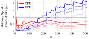
We further motivate the use of StridedBatchedGemm evaluations by plotting the speedup of the conventional approach – transpositions until a single Gemm can be called – over a single StridedBatchedGemm call in evaluation of Case 1.3 from Table II for tensors of size $\mathbf{n}\times\mathbf{n}\times\mathbf{n}$. Figure 3 shows that StridedBatchedGemm is significantly faster than performing even a single transposition followed by a flattened Gemm, especially for small matrices. Here, a single transposition means $\mathbf{n}$ calls to mkl_somatcopy on CPU or cublasSgeam on GPU in order to fully exchange two modes. The dark lines include only a single transposition and the lighter lines include 2, 3, and 6 transpositions.

On CPU, the StridedBatchedGemm evaluation outperforms the conventional approach for all $\mathbf{n}<512$. On GPU, the benefit from performing a single flattened Gemm eventually outweighs the cost of performing the transposition and for $\mathbf{n}\gtrsim 200$ the conventional approach achieves a speedup over the StridedBatchedGemm. This speaks to the highly optimized Gemm in CuBlas and that, perhaps, additional optimization gains from CuBlas’s BatchedGemm may be available.

IV-B Extended BLAS Evaluation

In this section, we compare evaluation strategies given the extended Blas kernels. On GPU, the StridedBatchedGemm interface is provided by modifying cublasSgemmBatched from CuBlas 7.5. On CPU, the StridedBatchedGemm interface is implemented in serial with looped calls to cblas_sgemm from Mkl 11.2. Both implementations thereby avoid additional allocation and/or precomputation at the call site. The serial execution on CPU emphasizes the cache effects discussed in the following sections.

IV-B1 Flattening

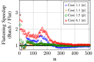
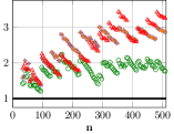
Cases 1.1, 1.5, and 6.1 can be evaluated without explicit transpositions with either a single flattened Gemm or a single BatchedGemm. We expect the flattened Gemm evaluation to outperform the BatchedGemm evaluation due to the optimization level of existing Gemms over that of the recently emerging BatchedGemm functions.

In Figure 4, we plot the speedup achieved by using a flattened Gemm evaluation over a StridedBatchedGemm evaluation. In Figure 4, the speedup is greater than one when FlattenedGEMM is faster than the StridedBatchedGemm. Clearly, most of the time, flattened Gemm is faster. Furthermore, we note the CuBlas implementation of StridedBatchedGemm is a great candidate for optimization as it appears to be significantly underperforming with respect to Gemm.

We also note the dependence of the performance on the shape of the flattened Gemm and the mode of the StridedBatchedGemm. On CPU, we find that the major determining factor in performance is the batching mode of the output. That is, the StridedBatchedGemm evaluation performs best when batched in the third mode of $C$ – in Case 1.5 $[p]$ and 1.1 $[p]$. On GPU, the output batching mode makes no difference. It is unclear why the batched evaluation performs so well on Case 1.5 $[p]$.

Figure 4: Performance ratio for a BatchedGemm over a flattened Gemm in evaluation of Cases 1.1, 1.5, and 6.1. (Left) CPU. (Right) GPU.

IV-B2 Batching

In this section, we attempt to quantify the performance gain by batching in the last mode versus an earlier mode and whether the input tensor or the output tensor should be prioritized for this optimization.

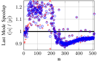
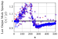
Case 1.1 and 2.1 can both be batched in the second ($[n]$) or third ($[p]$) mode. In Figure 5, we plot the speedup in performing the BatchedGemm in $[p]$ over performing it in $[n]$. When the size of the tensor is small, $\mathbf{n}\lesssim 256$, batching in the third mode is advantageous and can result in up to 1.25x speedup on CPU. When $\mathbf{n}\gtrsim 256$, it is approximately 1.1x faster to batch in the second mode rather than the third. We expect this is an effect of the 256KB L1 cache, which would house the contiguous $B_{kn}$ submatrix for each $p$ when $\mathbf{n}\lesssim 256$. Beyond that size both batching strategies will have forced cache misses within each Gemm, but by batching in the middle mode more data is shared between individual Gemms.

On GPU, we see no discernible preference in the choice of batching mode. The GPU has a much less sophisticated memory system with no prefetcher and the performance difference is primarily determined by the number of global memory transactions issued. When $\mathbf{n}\geq 32$, the coalescing width is reached so nearly the same number of transactions will be issued in each case – with small differences caused by alignment. We confirmed this by profiling the number of global memory reads and writes issued by each kernel and verifying that they correlate with the small differences in performance observed.

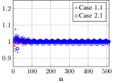
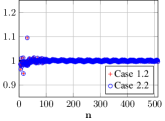
Additionally, we consider the mixed-mode batching evaluations to determine if the input or output array is the primary determination of batching performance. In Figure 6, we plot the speedup in performing StridedBatchedGemm in the last mode of the output but the middle mode of the input, $[p]$, over performing it in the middle mode of the output and the last mode of the input, $[n]$, for Cases 1.2 and 2.2. The results are very similar to those of Figure 5 indicating that batching mode of the output tensor $C$ is more important than the batching mode of the input tensor $B$ on CPU. This is consistent with reference implementations of Gemm which accumulate results directly into the output matrix.

Figure 5: Speedup obtained from batching in the last mode, $[p]$, rather than the middle mode, $[n]$, for Cases 1.1 and 2.1. (Left) CPU. (Right) GPU.

Figure 6: Speedup obtained from batching in the last output mode, $[p]$, rather than the middle output mode, $[n]$, for Cases 1.2 and 2.2. (Left) CPU. (Right) GPU.

IV-B3 Exceptional Cases

Figure 7: GPU tiling parameter profile from PPCG on K40c for Case 6.4. Performance values are $\log_{10}([\mu sec])$ and tests performed for $\mathbf{m}=\mathbf{n}=\mathbf{k}=\mathbf{p}=256$. White indicates the run failed.

Figure 8: Benchmark of three evaluation strategies for Case 6.4: A BatchedGemv, a mode transposition followed by a BatchedGemm, and an extended transpose kernel generated by PPCG.

In this section, we demonstrate the feasibility of evaluation strategies for the exceptional cases.

The Polyhedral Parallel Code Generator (PPCG) [28] is a source-to-source compiler capable of generating CUDA kernels from nested control loops in C. We use PPCG to generate a CUDA kernel for exceptional Case 6.4 and compare its performance against other evaluation strategies.

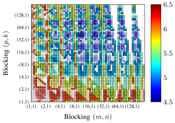
First, Case 6.4 has four nested loops and PPCG accepts a tiling parameter for each. We search the parameter space $(m,n,p,k)\in[1,2,4,8,16,32,64,128]^{4}$ for the most efficient variant in Figure 7. The kernels were generated with $\alpha=1$ and $\beta=0$ statically known as generated versions with dynamic $\alpha,\beta$ had significant branching and divergent overhead, whereas we are primarily interested in the access patterns and tiling.

The tiling parameters that result in the highest performance are $(16,4,32,4)$. Via inspection, we verify that the generated kernel is performing a 2D shared memory tiling for $A$, a “3D” shared memory tiling for $B$, and accumulating the $C$ results in registers.

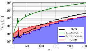
Using the $(16,4,32,4)$ kernel, we benchmark against two possible evaluation strategies: (1) A BatchedGemv which requires no explicit transposition, and (2) A mode transposition in $k$ and $m$ followed by a BatchedGemm in $[n]$. In Figure 8, we show the execution time for each with the explicit transposition/Gemm stacked to show their relative proportion in the two-step evaluation. The PPCG kernel outperforms the explicit transposition/Gemm evaluation for small matrices and remains within a factor of 2-3x as $\mathbf{n}$ grows. We expect an expert implementation of the extended transpose parameter kernel would be able to close this gap and remain competitive with BatchedGemm for all $\mathbf{n}$.

IV-C Machine Learning Application

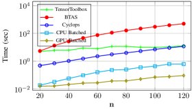
In this section, we present the benchmarking results for the application that we discussed in Section II-C. For simulations on the CPU, we compare the performance on the Tucker decomposition using TensorToolbox, Btas, Cyclops and our StridedBatchedGemm. For simulations on the GPU, we don’t have available GPU library to compare with, so we just evaluate our GPU implementation against StridedBatchedGemm. We fix the number of iterations as $\mathcal{T}=200$, set the core tensor size as $\mathbf{i}=\mathbf{j}=\mathbf{k}=10$, and set the dimensions as $\mathbf{m}=\mathbf{n}=\mathbf{p}$. From Figure 9, using our CPU StridedBatchedGemm, we obtain more than 10 times speedup compared to Cyclops/TensorToolbox and almost four orders of magnitude compared to Btas. Also, as expected, our GPU StridedBatchedGemm confers further speedup.

Figure 9: Performance on Tucker decompostion.

IV-D Evaluation Priorities

Rather than attempt to model the algorithm and machine as in [22, 19], we simply provide evaluation guidelines based on the data provided. These are a number of heuristics that may be important in constructing the most efficient evaluation strategy.

1. Flatten modes whenever possible. A single large Gemm is more efficient.

2. In the interest of performing the highest intensity computation within a BatchedGemm, we recommend performing the largest Gemms possible within a BatchedGemm and batching in the mode with largest dimension.

3. Preferring to batch in the last mode versus earlier modes can depend on the input parameters and machine.

We summarize these evaluation guidelines with pseudocode for performing a single-index tensor contraction without copy or transposition in Algorithm 2.

V Conclusions and Future Work

Our experience reveals that the emergence of BatchedGemm provides significant computational advantages for multi-linear algebraic computations. The primitive allows us to push a larger high intensity computations to vendor-provided implementations. Leading implementations already provide BatchedGemm on highly parallel machines. To simplify their use and provide additional optimization opportunities, we propose StridedBatchedGemm and demonstrate its use for generalized tensor contractions. Calls to StridedBatchedGemm have significant opportunity to perform at or near the performance of Gemm and, by avoiding explicit transpositions or permutations of the data, accelerate these computations significantly.

Our improvement is most significant on small and moderate sized tensors. This is very important because in many applications, e.g. deep learning for training a recursive tensor network, we require evaluating a large number of tensor contractions of small sizes.

Although we focused on single-node performance, these evaluations may be used as building blocks for distributed memory implementations, which we intent to pursue as part of our future work. Further study into the optimized implementations, architecture-dependent implementations, and performance of the exceptional case kernels is warranted. More complicated contractions, such as multi-index contractions or sparse tensor algebra, also pose challenging problems.

1:  In: Tensor $A_{\mathcal{A}}$, $\mathcal{A}=[a_{1},\dots,a_{M}]$,

2:  In: Tensor $B_{\mathcal{B}}$, $\mathcal{B}=[b_{1},\dots,b_{N}]$, $\mathcal{A}\cap\mathcal{B}=\{k\}$.

3:  In, Out: Tensor $C_{\mathcal{C}}$, $\mathcal{C}=[c_{1},\ldots,c_{N+M-2}]$. WLOG, $c_{1}\in\mathcal{A}$.

4:  Common substrings in $\mathcal{A}$, $\mathcal{B}$ and/or $\mathcal{C}$ for flattening candidates.

5:  Relabel flattened modes

6:  Compute $\mathcal{P}=\{c_{i}\ |\ i\neq 1,c_{i}\not\equiv a_{1},c_{i}\not\equiv b_{1}\}$

7:  if $\left|{\mathcal{C}\setminus\mathcal{P}}\right|=\left|{\{c_{1}\}}\right|=1$. then

8:     [Case $C_{c_{1}\cdots}=A_{k\cdots c_{1}\cdots}B_{k\cdots}$]

9:     Let $c^{*}\in\mathcal{P}\setminus\mathcal{A}$ be index with max dimension

10:     Let $c^{+}\in\mathcal{P}\setminus\{c_{1},c^{*}\}$ be index with max dimension

11:     Nested in all $c_{j}\in P\setminus\{c^{*},c^{+}\}$, BatchedGemm in $c_{1},c^{*},k,[c^{+}]$

12:  else if $\left|{\mathcal{C}\setminus\mathcal{P}}\right|=\left|{\{c_{1},c_{b}\}}\right|=2$ then

13:     [Case $C_{c_{1}\cdots c_{b}\cdots}=A_{k\cdots c_{1}\cdots}B_{c_{b}\cdots k\cdots}$]

14:     Let $c^{*}\in\mathcal{P}$ be index with max dimension

15:     Nested in all $c_{j}\in P\setminus\{c^{*}\}$, BatchedGemm in $c_{1},c_{b},k,[c^{*}]$

16:  else if $\left|{\mathcal{C}\setminus\mathcal{P}}\right|=\left|{\{c_{1},c_{a}\}}\right|=2$ then

17:     [Case $C_{c_{1}\cdots c_{a}\cdots}=A_{c_{a}\cdots c_{1}\cdots k\cdots}B_{k\cdots}$]

18:     Let $c^{*}\in\mathcal{P}\setminus\mathcal{A}$ be index with max dimension

19:     Nested in all $c_{j}\in P\setminus\{c^{*}\}$, Ex. BatchedGemm in $c_{1},c^{*},k,[c_{a}]$

20:  else if $\left|{\mathcal{C}\setminus\mathcal{P}}\right|=\left|{\{c_{1},c_{a},c_{b}\}}\right|=3$ then

21:     [Case $C_{c_{1}\cdots c_{a}\cdots c_{b}\cdots}=A_{c_{a}\cdots c_{1}\cdots k\cdots}B_{c_{b}\cdots k\cdots}$]

22:     Nested in all $c_{j}\in P$, Ex. BatchedGemm in $c_{1},c_{b},k,[c_{a}]$

23:  end if

Algorithm 2 Single-Mode Tensor Contraction

References

- [1] G. Baumgartner A. Allam, J. Ramanujam and P. Sadayappan. Memory minimization for tensor contractions using integer linear programming. IPDPS’06, 2006.
- [2] M. Abadi et al. TensorFlow: Large-scale machine learning on heterogeneous systems. Software available on tensorflow.org.
- [3] Baboulin M. Dobrev V. Dongarra J. Earl C. Falcou J. Haidar A. Karlin I. Kolev Tz. Masliah I. Tomov S Abdelfattah, A. High-performance tensor contractions for gpus. ICCS’16.
- [4] A. Anandkumar, R. Ge, D. Hsu, S.M. Kakade, and M. Telgarsky. Tensor decompositions for learning latent variable models. JMRL, 15(1):2773–2832, 2014.
- [5] Brett W. Bader and Tamara G. Kolda. Algorithm 862: MATLAB tensor classes for fast algorithm prototyping. ACM Trans. Math. Softw., 32(4):635–653, 2006.
- [6] Brett W. Bader, Tamara G. Kolda, et al. Matlab tensor toolbox version 2.6. Available online, http://www.sandia.gov/~tgkolda/TensorToolbox/, February 2015.
- [7] R. Bro and H. A. Kiers. A new efficient method for determining the number of components in parafac models. Journal of chemometrics, 17(5):274–286, 2003.
- [8] Aydin Buluç and John R Gilbert. The combinatorial blas:design, implementation, and applications. IJHPCA’11.
- [9] N. Goyal, S. Vempala, and Y. Xiao. Fourier pca and robust tensor decomposition. In Proceedings of the 46th Annual ACM Symposium on Theory of Computing, pages 584–593.
- [10] R.A. Harshman. Foundations of the parafac procedure: Models and conditions for an explanatory multi-model factor analysis. UCLA Working Papers in Phonetics, 16:1–84, 1970.
- [11] Frank L Hitchcock. The expression of a tensor or a polyadic as a sum of products. J. of Math.and Physics, 6(1):164–189, 1927.
- [12] C. Jhurani and P. Mullowney. A GEMM interface and implementation on NVIDIA GPUs for multiple small matrices. J. of Parallel and Distributed Computing, 75:133–140, 2015.
- [13] V. Kazeev, M. H. Khammash, M. Nip, and C. Schwab. Direct solution of the chemical master equation using quantized tensor trains. ETH-Zürich, 2013.
- [14] V. Khoromskaia and B. N Khoromskij. Tensor numerical methods in quantum chemistry: from hartree–fock to excitation energies. Physical Chemistry Chemical Physics, 2015.
- [15] L. Lathauwer, B. Moor, and J. Vandewalle. On the best rank-1 and rank-(,r2,…rn) approximation of higher-order tensors. SIAM J. Matrix Anal. Appl., 21:1324–1342, 2000.
- [16] J. Li, C. Battaglino, L. Perros, Ji. Sun, et al. An input-adaptive and in-place approach to dense tensor-times-matrix multiply. In SC’15, pages 76:1–76:12.
- [17] Q. Lu, X. Gao, et al. Empirical performance model-driven data layout optimization and library call selection for tensor contraction expressions. J. Parallel Distrib. Comput., 72(3):338–352, Mar 2012.
- [18] N. Nakatani, B. Verstichel, G. Chan, J. Calvin, et al. Btas v0.0.1. Available online, https://github.com/BTAS/BTAS.
- [19] E. Di Napoli, D. Fabregat-Traver, G. Quintana-Ortí, and P. Bientinesi. Towards an efficient use of the BLAS library for multilinear tensor contractions. AMC, 235:454 – 468, 2014.
- [20] T. Nelson, A. Rivera, P. Balaprakash, et al. Generating efficient tensor contractions for gpus. ICPP’15.
- [21] E. Peise and P. Bientinesi. Performance modeling for dense linear algebra. In SC/12: High Performance Computing, Networking Storage and Analysis.
- [22] E. Peise, D. Fabregat-Traver, and P. Bientinesi. On the performance prediction of BLAS-based tensor contractions. In PMBS’15.
- [23] E. Solomonik, D. Matthews, J. R Hammond, and J. Demmel. Cyclops tensor framework: reducing communication and eliminating load imbalance in massively parallel contractions. In Parallel & Distributed Processing, pages 813–824, 2013.
- [24] G. Kolda Tamara and W. Bader Brett. Tensor decompositions and applications. SIAM Review, 51(3):455–500, Mar 2009.
- [25] Ledyard R. Tucker. Some mathematical notes on three-mode factor analysis. Psychometrika, 31(3):279–311, 1966.
- [26] Field G. Van Zee and Robert A. van de Geijn. Blis: A framework for rapidly instantiating blas functionality. ACM Trans. Math. Softw., 41(3):14:1–14:33, June 2015.
- [27] M. Alex O. Vasilescu and D. Terzopoulos. Multilinear analysis of image ensamble: Tensorfaces. ECCV’02.
- [28] S. Verdoolaege, J. C. Juega, and A.and others Cohen. Polyhedral parallel code generation for cuda. ACM Trans. Archit. Code Optim., 9(4):54:1–54:23, January 2013.