The Gaia-ESO survey: Hydrogen lines in red giants directly trace stellar mass

Red giant stars are perhaps the most important type of stars for Galactic and extra-galactic archaeology: they are luminous, occur in all stellar populations, and their surface temperatures allow precise abundance determinations for many different chemical elements. Yet, the full star formation and enrichment history of a galaxy can be traced directly only if two key observables can be determined for large stellar samples - age and chemical composition. While spectroscopy is a powerful method to analyse the detailed abundances of stars, stellar ages are the ”missing link in the chain”, since they are not a direct observable. However, spectroscopy should be able to estimate stellar masses, which for red giants directly infer ages provided their chemical composition is known.

Here we establish a new empirical relation between the shape of the hydrogen line in the observed spectra of red giants and stellar mass determined from asteroseismology. The relation allows to determine stellar masses and ages with the accuracy of 10-15%. The method can be used with confidence for stars in the following range of stellar parameters: $4000<T_{\rm eff}<5000$ K, $0.5<\log g<3.5$, $-2.0<$ [Fe$/$H] $<0.3$, and luminosities $\log L/L_{\rm Sun}<2.5$. Our analysis provides observational evidence that the H_α spectral characteristics of red giant stars are tightly correlated with their mass and therefore their age. We also show that the method samples well all stellar populations with ages above $1$ Gyr. Targeting bright giants, the method allows to obtain simultaneous age and chemical abundance information far deeper than would be possible with asteroseismology, extending the possible survey volume to remote regions of the Milky Way and even to neighbouring galaxies like Andromeda or the Magellanic Clouds already with present instrumentation, like VLT and Keck facilities.

1 Introduction

One of the key problems in stellar and galactic astrophysics is to determine the age of a star. The star formation history of a population or galaxy can be best traced if we know how to connect the chemo-dynamical data of stars to their formation time.

Age determinations for the Galactic field stars have traditionally been limited to stars on the upper main sequence and on the subgiant branch. The most convenient and widely-used approach relies on fitting stellar isochrones to the classical observables (e.g. $T_{\!\mbox{\scriptsize\em\rm eff}}$, $\log{g}$, and $[\rm{Fe}/\rm{H}]$) (Pont & Eyer 2004, Jorgensen & Lindegren 2005). To a lesser extent, empirically calibrated methods are used (Soderblom 2010, 2015). They rely on various observational findings, such as emission lines that are related to the chromospheric activity, the depletion of Li with stellar age as the convection zone of a star thickens, and surface rotation, which slows down with increasing age. For the cool main-sequence stars, more elegant and accurate adaptations of the rotation method have been proposed (Garcia et al. 2014, Meibom et al. 2015), but they also rely on ultra-precise light-curves.

For red giant stars, the stars of most prominent interest in the context of Galactic and extra-galactic archaeology, classical isochrone methods are not useful: even if the metal content is known, isochrones of different ages are very close and would require $T_{\!\mbox{\scriptsize\em\rm eff}}$ and $\log{g}$ determinations with better than $0.5$% accuracy. Only if luminosities of the stars are accurately known, e.g. because distances are available and reddening is not a problem, can evolutionary models be used to determine stellar mass (Ghezzi & Johnson 2015). However, also these determinations suffer from systematic errors in input stellar parameters and uncertainties of the stellar models. One may relate the process of ageing to in situ stellar nucleosynthesis, e.g. the ratio of carbon over nitrogen abundance increases as the star experiences multiple dredge-up episodes and the products of stellar nucleosynthesis are mixed to the surface (Masseron & Gilmore 2014, Martig et al. 2016, Ness et al. submitted).

Recently, asteroseismology has emerged as a promising tool to determine masses of stars that display solar-like oscillations, i.e. stochastic oscillations excited by turbulent motions in the stellar convective envelope. Asteroseismic observations provide the surface gravity and mean density of a star, and, in combination with $T_{\!\mbox{\scriptsize\em\rm eff}}$ and $[\rm{Fe}/\rm{H}]$, yield precise masses for stars of all types (Chaplin et al. 2014, Pinsonneault et al. 2014), from the main sequence (MS) through the hydrogen-shell-burning (RGB) to the core-helium burning (Red Clump, hereafter RC) phase. Asteroseismology is a very promising method, however it has two caveats. First, the accuracy of masses and ages derived depends on asteroseismic scaling relations. These relations may suffer from systematic biases of a few percent (e.g. Belkacem et al. 2011, Miglio et al. 2012, Coelho et al. 2015, White et al. 2015). Secondly, the method is mainly useful for sub-Galactic studies in the limited volume of the Milky Way, since the photometric data quality quickly deteriorates with magnitude and hence distance. Thus the technique cannot provide any mass or age estimates for larger distances, in- and outside the Galaxy.

The determination of the mass and composition of an evolved red giant star is, unlike for a main sequence star, an excellent proxy for its age. The time a star lives as a red giant is a small fraction of its total main sequence lifetime. The latter is determined through stellar evolutionary models by the initial mass and composition of the star. Then, the age of a red giant star is to a very good approximation only a function of those two quantities. If masses, or proxies for masses, can be estimated from observations, age-dating of giants is more straightforward than for main-sequence stars (Soderblom 2010).

Here we report on a newly observed relationship between the shape of the optical hydrogen line (H_α) and the mass of red giant stars. More massive stars appear to have fainter, i.e. weaker, H_α lines. We make use of high-resolution and high signal-to-noise spectra from different observational programs, including the Gaia-ESO large spectroscopic survey (Gilmore et al. 2012, Randich et al. 2013) and asteroseismic data from the CoRoT and Kepler space missions. Our approach is purely empirical. We cannot yet identify the physical mechanism underlying the relation, because there are no red giant model atmospheres built from first principles that could be used to reproduce the observed H_α line, to guide our understanding of the relationship with the stellar mass. The relationship, which we established on Galactic field stars, also gives accurate results for the stars in open and globular clusters, enabling direct spectroscopic stellar mass measurements without isochrone fitting.

The paper is structured as follows. Our observations and the data analysis are presented in Sec. 2, along with a brief summary of the state-of-the-art in modelling Balmer lines in the spectra of cool stars. The new method to derive masses and their implied ages is described in Section 3.2. In Sec. 5 we outline some applications of the method in the context of Galactic and extra-galactic astrophysics.

2 Observations and analysis

2.1 Spectroscopic observations

Our main dataset is the high-resolution stellar spectra from the Gaia-ESO 2nd and 3rd data releases (iDR2iDR3). The majority of the spectra have signal-to-noise (S/N) ratios between $50$ and $220$. In the top tier we have the stars with high-quality asteroseismic data from CoRoT, but we, too, include red giants observed in open and globular clusters (Table 1). The stars in clusters do not belong to our core dataset, though, since their masses and ages are determined by another method, the cluster colour-magnitude diagram (CMD) fitting. The data reduction of the UVES spectra has been described in Sacco et al. (2014) in detail. The radial velocity correction was performed masking the Balmer lines and regions affected by telluric contamination. The spectra were normalised by dividing them with a function, which describes the stellar continuum emission convolved with the FLAMES-UVES instrumental response as described in Sacco et al. (2014). In total, the Gaia-ESO sub-sample contains $21$ CoRoT stars in the Galactic field and $73$ stars in $7$ star clusters. The observational details are listed in Tables 3 and 5 in Appendix.

In addition, we include $47$ stars from Thygesen et al. (2012) that were observed by Kepler and included in the first APOKASC Catalog (Pinsonneault et al. 2014). The evolutionary status is known for some of them. The stellar spectra were taken on different facilities with resolving powers ranging from $67\,000$ (NOT) to $80\,000$ (NARVAL). The spectra are available from Thygesen et al. (2012). The S$/$N ratios are between $80-100$ to $200$. Our sample, too, includes two very metal-poor stars, KIC 4671239 (Hennes) and KIC 7693833 (Rogue). These objects are the targets of Silva Aguirre et al. (2016, in preparation). The spectrum of KIC 4671239 is now publicly available from the NOT database, and KIC 7693833 was observed by Thygesen et al. (2012). The data reduction of these spectra is described in Thygesen et al. (2012).

The full sample contains $69$ Galactic field stars with asteroseismic masses and $73$ stars in the clusters. Figure 1 shows the location of the stars on the Hertzsprung-Russell diagram. These are red giants or red clump stars with $T_{\!\mbox{\scriptsize\em\rm eff}}$  in the range $4000-5000$ K, and $\log$ g from $0.5$ to $3.6$. The stars span a wide range of metallicity from $-2.64$ to $0.5$.

For consistency, we renormalise all available spectra using the same procedure as in Schönrich & Bergemann (2014) that fits selected continuum windows with a low-order polynomial.

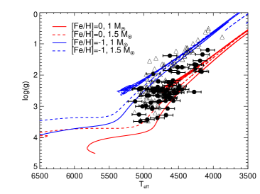
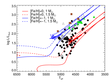
Figure 1: The Hertzsprung-Russell diagram for the observed stellar sample: black filled points - the stars with asteroseismic masses, triangles - the stars in stellar clusters. The stars in the globular clusters NGC 2808 and NGC 4372 are shown with green triangles and brown squares, respectively. The Garstec evolutionary tracks (Serenelli et al. 2013) for different masses and metallicities are also shown.

Table 1: Stellar parameters for star clusters. The references to metallicities and ages are also given.

Cluster	[Fe/H]	Age	Mass	Reference
	dex	Gyr	M$\odot$
M 67	0.06	4.30	1.32	Salaris et al. (2004)
NGC 2243	$-$0.48	4.66	1.20	Salaris et al. (2004)
NGC 5927	$-$0.50	10.75 $\pm$ 0.38	0.94	Vandenberg et al. (2013)
NGC 2808	$-$1.18	11 $\pm$ 0.38	0.84	Vandenberg et al. (2013)
NGC 1851	$-$1.18	11 $\pm$ 0.25	0.84	Vandenberg et al. (2013)
NGC 6752	$-$1.54	12.50 $\pm$ 0.25	0.79	Vandenberg et al. (2013)
NGC 4372	$-$2.17	11.2 - 12.5	0.81	De Angeli et al. (2005)

2.2 Model atmospheres and spectroscopic analysis

For the Gaia-ESO dataset, we use the recommended $T_{\!\mbox{\scriptsize\em\rm eff}}$  and [Fe/H] available from the iDR3 stellar parameter analysis run (Table 4). The stellar parameters values were determined as described in Smiljanic et al. (2014) and in Bergemann et al. (2014), using several different methods of spectroscopic analysis. The radiation transport is solved in LTE with MARCS model atmospheres (Gustafsson et al. 2008). The typical uncertainty in the parameter values is 100 K in $T_{\!\mbox{\scriptsize\em\rm eff}}$ and $0.1$ dex in $[\rm{Fe}/\rm{H}]$. For one of the NGC 4372 stars, 12253419-7235252, we adopt the following uncertainties: $\delta$ $T_{\!\mbox{\scriptsize\em\rm eff}}$$\leavevmode\nobreak\ =100$ K,  $\delta\log g=0.5$ dex, $\delta[\rm{Fe}/\rm{H}]=0.2$ dex, because no data is available in the survey database. The uncertainties are conservative and reflect the deviation of individual spectroscopic estimates. These uncertainties have a very small impact on the mass estimates: the 100 K error in $T_{\!\mbox{\scriptsize\em\rm eff}}$ propagates as a $5\%$ error in mass, and the error of $0.1$ dex in $[\rm{Fe}/\rm{H}]$ propagates as a 1.5% error in mass. The comparison with the independent photometric estimates gives us confidence in the the accuracy of stellar parameters. The spectroscopic $T_{\!\mbox{\scriptsize\em\rm eff}}$  estimates agree to better than $70$ K with the temperatures determined using the method of Infra-Red Fluxes Casagrande et al. (2014).

For the Thygesen et al. (2012) stellar sample, we use the values of $T_{\!\mbox{\scriptsize\em\rm eff}}$  and $[\rm{Fe}/\rm{H}]$ that were determined by Bruntt et al. (2012). The stellar parameters are provided in Table 7. One of the very metal-poor (VMP) stars, Rogue, has metallicity $[\rm{Fe}/\rm{H}]=-2.23$ and was analysed by Thygesen et al. (2012). For the other, Hennes, the mean of two values given in Silva Aguirre et al. (2016, in preparation) and used by Guggenberger et al. (in preparation) is $[\rm{Fe}/\rm{H}]=-2.64\pm 0.22$.

2.3 Asteroseismic data and analysis

Stellar masses are determined using the global seismic quantities, available from the CoRoT and Kepler space mission observations. For the Gaia-ESO stellar sample, the asteroseismic data taken from Mosser et al. (2010). The large frequency separation, $\Delta\nu$, is approximately the average frequency separation of radial oscillation modes of consecutive order. The second seismic quantity is $\nu_{\rm max}$, the frequency at which the oscillations power spectrum exhibits its maximum power. $\Delta\nu$ and $\nu_{\rm max}$ scale with global stellar parameters as

$$\frac{\Delta\nu}{\Delta\nu_{\odot}}\simeq\sqrt{\frac{M/{M_{\odot}}}{(R/{R_{\odot}})^{3}}},\ \ \ \frac{\nu_{\rm max}}{\nu_{\rm max}{{}_{\odot}}}\simeq\frac{M/M_{\odot}}{(R/{R_{\odot}})^{2}\sqrt{T_{\rm eff}/T_{\rm eff}{{}_{\odot}}}}.$$ (1)

For each star, $\Delta\nu$ and $\nu_{\rm max}$ together with $T_{\!\mbox{\scriptsize\em\rm eff}}$ and $[\rm{Fe}/\rm{H}]$ values (Section 2.2) are used as inputs to the BeSPP code (Serenelli et al. 2013), a Bayesian grid-based modelling algorithm for determination of fundamental stellar properties (mass, age, evolutionary stage). BeSPP uses a large grid of Garstec stellar evolutionary tracks ($6\times 10^{7}$ stellar models, $0.6\leq M/\leavevmode\nobreak\ M_{\odot}\leq 3.0$), from the pre-main sequence to the beginning of the thermal pulses on the asymptotic giant branch (Weiss & Schlattl 2008). The posterior probability of each model is constructed as the product of the likelihood of the observables given the model and a set of prior probabilities related to the initial mass function, star formation rate and age-metallicity relation (see Serenelli et al. 2013, for details). The evolutionary state of stars, when known as it is the case for some stars in Thygesen’s sample, is also added as a binary prior. The full probability distribution function is then marginalised to obtain the posterior probability distributions for stellar mass and age. For the VMP stars, Rogue and Hennes, we use the best available asteroseismic masses (Silva Aguirre et al. 2016, in preparation), where a new version of the scaling relations by Guggenberger et al. (in preparation) was employed. We use their results, because the validity of standard scaling relations at low metallicity is currently under debate (Epstein et al. 2014).

2.4 State-of-the-art in modelling H_α  spectra of cool stars

It is well-known that strong spectral lines, including the H_α, Mg II UV doublet, and Ca II near-IR triplet cannot be fit in the spectra of cool stars with the classical models of stellar photospheres, i.e. the models based on the standard assumptions of 1D hydrostatic equilibrium and LTE (Rutten 2008; Rutten & Uitenbroek 2012, and references therein).

To illustrate the problem, we show the observed and synthetic line profiles for the two reference stars, the Sun (KPNO FTS atlas) and HD 122563 (the UVES POP spectrum, Bagnulo et al. 2003) in Fig. 2. The model spectra were computed in LTE using the broadening theory of Barklem et al. (2000) using the time- and spatially-averaged 3D hydrodynamical models from the Stagger grid (see Collet et al. 2011, Bergemann et al. 2012, Magic et al. 2013a,b) and the MARCS models (Gustafsson et al. 2008). In both cases, the models fail to describe the observed line shape: the observed profile is stronger than the best-fit model. The plot also shows non-local thermodynamic equilibrium (NLTE) line profiles computed using the H model atom from Mashonkina et al. (2008). While NLTE radiation transport does improve the fit in the H_α core, the model line is still too narrow compared to the observed data.

Remarkably, every RGB and RC star in the sample suffers from a similar systematic offset. Figure 3 compares the observed equivalent widths (EWs) of the H_α line for our stellar sample with asteroseismic masses (Section 2.1) with the best-fit 1D and average 3D model atmospheres. Comparison with the observed EWs shows a much greater than expected spread of the line strengths: the differences amount to almost $\sim 700$ mÅ  for the coolest stars, i.e. more than a $50$% error. The error shows a striking correlation with the surface stellar parameters, the effective temperature and surface gravity. Taking into account the mean 3D structures (Fig. 3, bottom panel) does not improve the agreement with the H_α observations suggesting that some other physical process is needed to explain the data.

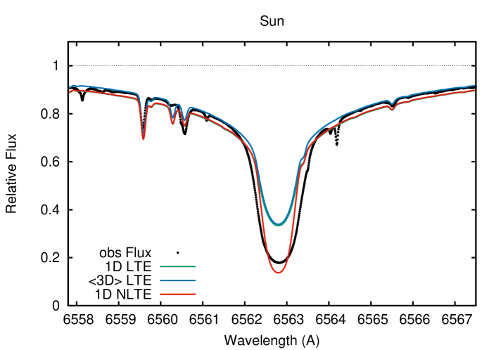
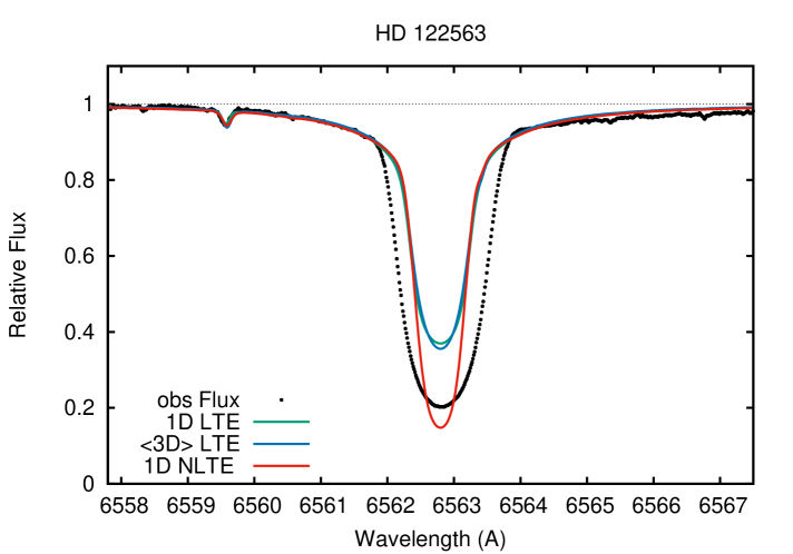
Figure 2: Model line profiles (colour lines) computed with different physics (1D LTE, mean 3D LTE, 1D NLTE) in comparison with the observed spectrum of the Sun (dots, top) and the metal-poor red giant HD 122563 (dots, bottom). The models lie far away from the data, thus we resort to an empirical method (Sect. 2.5).

While the systematic discrepancy has been known for decades, the methodological strategies to improve the models have been quite fragmented so far. Dupree et al. (1984) were among the first to suggest that adding chromospheres and mass flows to the 1D static model photospheres in the framework of ”extended atmosphere models” may work for cool stars. Such semi-empirical models assume that the chromospheres are excited by magnetic and mechanical disturbances propagating as electromagnetic-hydrodynamical waves (Alfvén 1942, Babcock 1961, Hartmann & McGregor 1980). The deposition of energy and momentum due to shock waves defines chromospheric energy balance, thus, at the very least, incident wave energy flux and the magnetic field are needed to compute the model. The ability of such models to fit the observed stellar spectra, however, critically depends on the availability of additional information. The observed H_α line profiles in the stellar spectra are used to iteratively constrain the free parameters, including the temperature (hereafter, $T$)-depth slope, the location of the $T$ minimum, and the velocity field (Meszaros et al. 2009; Dupree et al. 2016). All these parameters can not yet be calculated from first principles: in particular, the choice of the profile of turbulent velocity with depth is essential to fit the H_α width (Dupree et al. 2016). Moreover, one essential ingredient in the chromospheric models is NLTE radiation transport, since under the LTE assumption the line source function couples to the outwardly increasing temperature and causes an unphysical emission in the line cores (Przybilla & Butler 2004).

Rutten & Uitenbroek (2012) explored the formation of the solar H_α line using the 1D solar plane-parallel Kurucz model atmosphere and the semi-empirical solar chromospheric model by Fontenla et al. (2009). Their results (see their Fig. 8) suggest that NLTE radiation transport and chromospheric back-radiation are two necessary, albeit not sufficient, ingredients to describe the H_α profile. Indeed, while the Kurucz (Kurucz 1979) model predicts too narrow H_α line cores, in the model with an overlying (but empirically constrained) chromosphere the H_α core forms much higher in the atmosphere and is more opaque. On the other hand, their best model also produces too little opacity in the H_α core to fit the observed solar spectrum, similar to what is shown in Fig. 2 (top panel), although the NLTE line centre intensity (at 6562.8 Å) is closer to the observational data. A similar approach has been explored by Przybilla & Butler (2004), who showed that the irradiation of the inner photospheric layers by the chromosphere does little for the H_α profile in the solar spectrum (their Fig.2, top panel). Remarkably, four different solar model atmospheres, with and without chromospheres, produce essentially identical NLTE H_α profiles, challenging the argument that chromospheres are essential in describing the H_α line shapes. Thus, apart from the conceptual difficulty with computing chromospheres from first principles, it is still unclear what effect do chromospheres have on the stellar H_α lines. Disconcerting as it may be, as such, the 1D static or dynamical models with parametrised chromospheres do not yet offer a suitable framework for the quantitative analysis of H_α profiles in stellar spectra.

Figure 3: Comparison of the observed and synthetic equivalent widths of the H_α  line for the reference asteroseismic stellar sample. See Sect 2.4 for more detail.

More advanced 3D radiation magneto-hydrodynamic (MHD) simulations of chromospheres have been developed only recently (Carlsson & Stein 2002, Hansteen 2004, Gudiksen et al. 2010, Leenaarts 2010, Hansteen et al. 2015). The models are clearly more physically realistic than the 1D or 2D implementations, however, at present their applicability to other stars than the Sun remains questionable, since the simulations are, too, parametrised and require making use of spatially-resolved stellar observations, such as those provided by the MDI instrument for the Sun (Leenaarts et al. 2012). Also, there are still some open issues that pose a challenge to the simulations (Leenaarts 2010). First, the MHD models combined with the Hinode/SOT Ca II observations of the Sun predict that the power in acoustic waves is far too small to explain the chromospheric radiative energy losses (Carlsson et al. 2007). Second, fitting the H_α core with the MHD simulations has traditionally been problematic, because of the missing H_α opacity in the chromosphere. Leenaarts et al. (2012, 2015) showed that including non-equilibrium ionisation of hydrogen in the calculations of the equation-of-state in the 3D MHD models could help to resolve the long-standing disagreement with the H_α line-core imaging observations of the Sun. The simulations show that the opacity in the outer H_α core is correlated with the gas temperature, while the opacity in the inner core is mostly sensitive to the gas density. However it remains yet to be investigated whether the MHD models with prescribed radiative cooling rates (from the 1D chromospheric simulations that is only computationally tractable presently) describe the observed solar H_α line profile shape, not only the monochromatic brightness contrast across small areas on the solar surface. Finally, the 3D MHD chromospheric simulations for stars other than the Sun are currently not available, therefore neither quantitative nor qualitative statements about the behaviour of H_α lines in other stars, especially those with very different interior properties, such as RGB or RC, can be made.

2.5 Empirical fits to the H_α  profile

As discussed in the previous section, it is presently not possible to construct a grid of stellar atmosphere models that include all the sophisticated physical processes needed to describe the hydrogen line profiles in the observed spectra of RGB and RC stars. On the other hand, the obvious systematic misfit in the H_α line (Figs. 2, 3) is puzzling and it has prompted us to take a different, empirically motivated, approach to the problem. We ask whether there is a mathematical function that fits the H_α line profiles in the spectra of all our sample stars.

Since the red wing of the H_α  line is blended by a metallic feature (the line of neutral cobalt), we focus on the unblended left side of the core of the line, as shown by arrows in Fig. 5. The line mask is the same for all stars, it covers the wavelength range $6562.0-6562.8$ Å. By selecting this mask, we ensure that the Co I blend has no effect on the fit. The left limit at 6562.0 Å is set to minimise the contribution of the Si I and Fe I blends. None of the stars in the sample show evidence of emission in the wings or significant core shifts that could introduce spurious artefacts in the fit. Such features are usually seen in the spectra of metal-poor, $[\rm{Fe}/\rm{H}]<-1$, red giants brighter than $\log L/L_{\odot}\sim 2.5$ (Cacciari et al. 2004; Meszaros et al. 2009), while all but two of our reference stars with asteroseismic masses are fainter than this luminosity threshold (Fig. 1). We also do not see signatures of emission or line core shift in the most metal-poor stars in our sample, e.g. KIC 7693833, KIC 8017159 (Fig. 5).

We have explored different functions and find that the observed blue wing of the H_α line is well described by a cubic exponential function:

$$f(\lambda)=1-f_{0}\cdot\exp(-\left(|\lambda-\lambda_{0}|/W_{H_{\alpha}}\right)^{3})$$ (2)

where $\lambda_{0}$ is the central wavelength of the line, $6562.819$ Å (Baker 2008) and is fixed, $f_{0}$ the minimum flux in the line core, and $W_{H_{\alpha}}$ - a free parameter which correlates with the width of the spectral line and, as it will be shown later, with the mass of a star. It is important to stress that this is a purely mathematical function that has no input from the stellar atmosphere models or instrumental effects, such as the spectrograph line spread function. For our spectra, the resolving power is so high that the latter effects do not matter. However, for low-resolution spectra, values of $W_{H_{\alpha}}$ derived from different observational set-ups can not be compared directly. The free parameters to be fit to an observed profile are the line depth parameter, $f_{0}$, and the line width parameter, $W_{H_{\alpha}}$; their measured values for the full stellar sample are given in Tables 4,6,7. The uncertainty of the fitting is determined by shifting the continuum by $\pm 2\sigma$ from the best-fit solution and repeating the function fit. The difference with the best-fit normalisation then gives the uncertainty in the $W_{H_{\alpha}}$ estimate, which for all stars in the sample is below $0.01$ Å. It is thus reasonable to adopt the same error of $W_{H_{\alpha}}$ for all stars.

Figure 5 compares the function fit from the Eq. 2 with the observed H_α line profiles in several program stars. The theoretical line profiles computed in 1D LTE and NLTE are also shown.

Line bisectors, included in the plot insets, help to understand how the observed H_α shape changes as a function of stellar parameters. The bisectors were computed by dividing the spectral line into $15$ segments. Then the bisector velocity $v_{\rm bis}$ was estimated at full width at half-maximum of the line profile, as the wavelength shift relative to the central H_α wavelength. The Co I blend at 6563.42 Å, which is very strong in the solar metallicity giants ($[\rm{Fe}/\rm{H}]>-1$), causes an inverse $c$-shaped bisector profile (Figure 5, bottom panels), with $v_{\rm bis}$ up to 2 km$/$s. In the low-metallicity spectra, $[\rm{Fe}/\rm{H}]<-2$, the behaviour is inverted and the bisector profile has a $c$-shape. The bisector velocity measurements for the full asteroseismic sample are shown in Fig. 4. The line blending explains why the bisector velocity $v_{\rm bis}$ shows a strong correlation with $[\rm{Fe}/\rm{H}]$. We stress, though, that we fit only the blue part of the H_α core, so that the Co blend in the red wing has no effect on the $W_{H_{\alpha}}$ measurements.

Figure 4: Bisector velocity at the FWHM of the H_α profile (km$/$s) as a function of metallicity $[\rm{Fe}/\rm{H}]$ for the observed stellar sample.

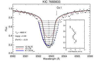
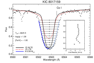
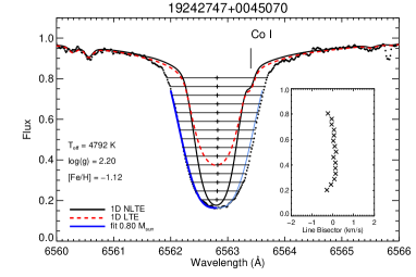
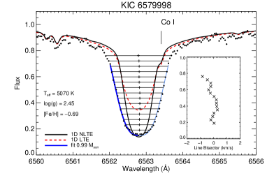
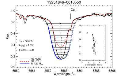
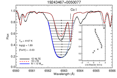
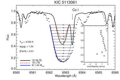
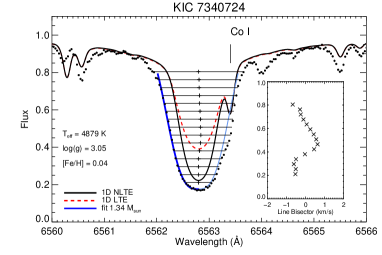
Figure 5: The observed H_α  profile (black dots) in the selected program stars and the best-fit empirical model from the eq. 2 (bold blue line, $6562.0$ to $6562.8$ Å). The red and black lines correspond to the best-fit theoretical models computed in 1D LTE respectively 1D NLTE. The part of the H_α line used in the fit is the same for all stars in the sample. The thin blue line is shown to help guide the eye only - the red wing of H_α is not used in the fit. Line bisectors are indicated in the inset. The spectra are arranged in order of increasing metallicity.

It should be noted that the H_α line develops strong wings in stars hotter than about $4900-5000$ K, depending on metallicity; this is the temperature limit where interactions with ions, electrons, and hydrogen atoms become important leading to the specific profile shape with self-broadening, van der Waals, and Stark damping wings. Thus, the simple shape, as described by the cubic exponential function may not apply, and caution is advised when fitting the Eq. 2 to the spectra of lower RGB or subgiant branch stars.

3 Results

3.1 H_α and stellar parameters

We have explored the correlation of the measured H_α line properties with different stellar parameters. The results for our reference asteroseismic sample and for the stars in the clusters are shown in Fig. 6. In the $[\rm{Fe}/\rm{H}]-W_{H_{\alpha}}$ plot, only the mean values of the measured cluster metallicity and $W_{H_{\alpha}}$ are shown, because the observed scatter in $[\rm{Fe}/\rm{H}]$ (as seen in Table 6) could be caused by the measurement uncertainties.The error bars show $1\sigma$ standard deviation of the individual $W_{H_{\alpha}}$ measurements within each cluster.

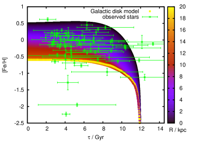
Figure 13: The age-metallicity relation (AMR) for our observed stellar sample in the Milky Way disk, computed using the asteroseismic masses and spectroscopic metallicities. The AMR for different Galactocentric radii (R in kpc) from a chemical evolution model of the Galactic disk (Schönrich & Binney 2009) is represented by the colour map.

The plots show that there is no clear dependence on $T_{\!\mbox{\scriptsize\em\rm eff}}$, but there are correlations between $W_{H_{\alpha}}$ and $\log g$, as well as between $W_{H_{\alpha}}$ and metallicity. The more metal-rich stars appear to have narrower H_α lines (smaller $W_{H_{\alpha}}$), as opposed to the more metal-poor stars, which show broader H_α profiles and, thus, lie at large values for $W_{H_{\alpha}}$. This correlation with metallicity is interesting, because it already looks quite similar to a classic age-metallicity relation (Fig. 13 in the Appendix). Also, given the $W_{H_{\alpha}}$ - metallicity correlation, it is also not surprising to find the correlation of $W_{H_{\alpha}}$ with asteroseismic $\log g$. Surface gravity depends on the star’s mass and radius, thus this correlation may indicate there is a more fundamental underlying relationship, such as that with stellar mass.

The stars in NGC 2808 ($[\rm{Fe}/\rm{H}]=-1.11$) show the largest intra-cluster spread of the $W_{H_{\alpha}}$ estimates that is reflected in the large uncertainty of its mean value. The most metal-poor cluster NGC 4372 ($[\rm{Fe}/\rm{H}]=-2.20$), too, stands out in the $W_{H_{\alpha}}-[\rm{Fe}/\rm{H}]$ plot. The only noteworthy difference of the NGC 2808 and NGC 4372 stars with respect to the other clusters is their comparatively high luminosity (Fig. 1): most of the observed stars in these two clusters have $\log L/L_{\odot}\geq 2.5$, which is where one could expect the effect of asymmetries and periodic variations in the H_α profile to become important (Cacciari et al. 2004, Meszaros et al. 2009). However, visual inspection of the observed data did not reveal any obvious problems with the spectra. Neither do we have repeated observations of these stars to check the effect of variability. Thus, currently, we do not have a suitable explanation for the behaviour of $W_{H_{\alpha}}$ in the most luminous stars in the globular clusters and set it aside as a problem to be addressed in future work.

Figure 6: The H_α width parameter measurements in the observed stellar sample versus stellar effective temperature, surface gravity, and metallicity. The stars with asteroseismic data are shown with filled circles and the stars in the clusters with filled triangles.

3.2 Mass effects in the Balmer line

While the $W_{H_{\alpha}}$ vs. $[\rm{Fe}/\rm{H}]$ and $\log g$ plots already suggested that $W_{H_{\alpha}}$ is related to the mass and hence age of stars, we can directly probe this by plotting the dependence between $W_{H_{\alpha}}$ and the independently determined asteroseismic mass (Fig. 7). This correlation is well-defined and it appears that all stars, also those in star clusters, follow the same $W_{H_{\alpha}}$-mass trend within the errors. H_α lines tend to be narrower in the spectra of more massive stars, but broader in the spectra of less massive stars. All we now need for a mass estimate from spectroscopy is to fit a relationship between $W_{H_{\alpha}}$ and the independent mass determinations. For the sake of simplicity, we fit a linear relation between H_α and the logarithmic mass of stars in our sample, i.e. $\log{M}=a\cdot{W_{H_{\alpha}}}+b$. This is done by a $\chi^{2}$ fit to the bootstrapped data in order to avoid that a few stars with small mass uncertainties dominate the results. In addition, we find an almost perfect linear relation between $a$ and $b$. Thus, $b$ can in turn be expressed as a linear function of the slope $a$, with the advantage that the uncertainty of the fit can be expressed in terms of the uncertainty in $a$, determined from the bootstrapping. The final result is:

$$\log{M({\rm H_{\alpha}})}=a\cdot\left({W_{H_{\alpha}}}-0.73\right)+0.08;$$ (3)

where $a=-2.73\pm 0.72$. This is shown in Figure 7 as the black solid line. Dashed black lines show the 1$\sigma$ uncertainty of the fit, as obtained from the bootstrap analysis described above. The shaded area is the average root-mean-square difference between the data and the fit.

Fig. 8 (a) compares our empirical masses determined from the Eq. 3 with the reference asteroseismic masses for the program stars. Panel (b) shows the results from the classical ”stellar isochrone” approach that makes use of the stellar parameters from spectroscopy ($T_{\!\mbox{\scriptsize\em\rm eff}}$, $\log{g}$, $[\rm{Fe}/\rm{H}]$) and isochrones (Serenelli et al. 2013). The masses determined empirically from the H_α measurements are more precise compared to the classical stellar evolution approach. The plot, however, reveals that we are slightly over-estimating masses at the low-mass end, and under-estimating masses for more massive stars. At present, it is not clear what is the origin of this systematics - the asteroseismic estimates or some kind of a second parameter problem in H_α. More data will be needed to explore this differences. Taking into account the uncertainty in the $a$ coefficient, and by cross-validation with the reference asteroseismic masses, we conclude that the accuracy of our mass estimates is about $0.15$ M_⊙.

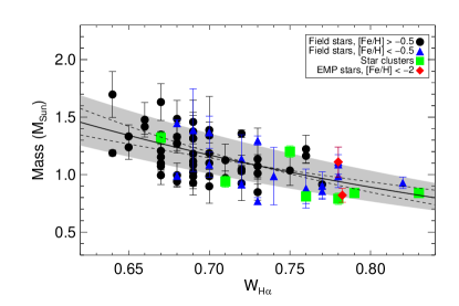
Figure 7: The observed relation between the H_α  spectral line widths versus asteroseismic masses of stars. Star clusters from the Gaia-ESO survey are shown with green diamonds. The very metal-poor stars in the sample, $[\rm{Fe}/\rm{H}]<-2$, are shown with red symbols. Dashed black lines show the 1$\sigma$ uncertainty of the fit. The shaded area is the average rms between the data and the fit. See Sect. 3.

3.3 Stellar ages

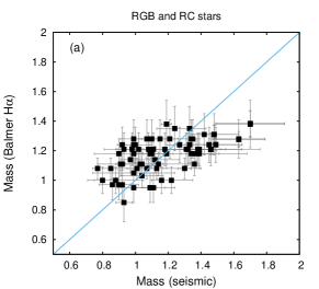
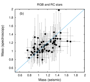
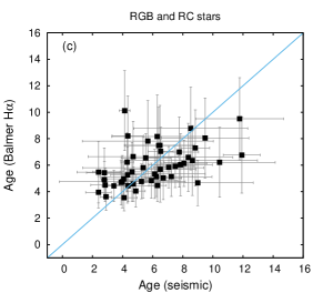
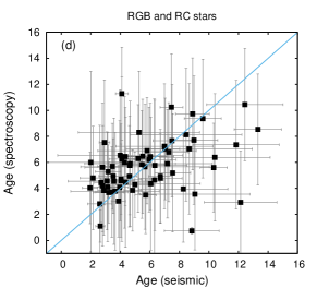
Figure 8: The comparison of masses (top panel) and ages (bottom panel) determined using the $W_{H_{\alpha}}$ coefficient directly (a,c) and the classical method of stellar isochrones (b,d).

In view of the relationship discussed above, another interesting point is whether the H_α line profiles show any evidence of ageing, i.e. a star getting older. This is unlikely, even though there is observational evidence that chromospheric activity decreases with stellar age (Steiman-Cameron et al. 1985). If true, one could see some effects in the observed stellar spectra, since the degree of line core filling by the chromospheric temperature inversion would change in lockstep with age. Younger and more active stars would show brighter line cores.

However, we can use a different approach. The initial mass and chemical composition are the two fundamental quantities needed to determine the age of red giant stars. One complication is a substantial mass loss: from observations only the present-day mass can be determined, while age estimates require knowledge of the initial mass of a star. Mass loss may affect the absolute ages of very evolved ($\log{g}\,\lesssim$ 1.5) low mass RGB and RC stars. This difficulty, however, is universally present in any method for determining the age of red giant stars based on their mass, including asteroseismology, and addressing it is outside of the scope of the paper. In this work, we want to understand whether stellar ages derived from the H_α width coefficient directly are consistent with the ages determined from asteroseismology, which is the best currently available method.

We use the masses determined from the H_α line width parameter (Eq. 2) and the Eq. 3 in BeSPP, the Bayesian grid-based modelling code (see Sect. 2.3). The resulting ages are shown in Fig. 8 (panel c) for the stars, for which we have confidence in the reliability of the H_α mass estimates (i.e. those with $T_{\!\mbox{\scriptsize\em\rm eff}}$$<4900$ K, Sect. 2.5). The age uncertainties are computed as $\pm 34\%$ around the median value. The very large errors of the ages determined with the classical method reflect the uncertainty of the input spectroscopic gravities, which are of the order $\sim 0.2$ dex.

Fig. 8 highlights the main problem of the classical mass and age determination on the RGB. In the standard isochrone fitting method (panels b,d of Fig. 8), the likelihood on the RGB is nearly flat, because all isochrones line up together. To distinguish stars with the age difference of even $10$ Gyr, extreme and so far unachievable precision in $T_{\!\mbox{\scriptsize\em\rm eff}}$  and $\log g$ ($10$ K and $0.02$ dex) is needed. In the Bayesian framework, the ages determined using uninformative data are completely dominated by the priors, especially the initial mass function (Serenelli et al. 2013, Fig. 4). For a simple stellar population, this approach may work producing an age distribution which does not look too odd, but just by chance. Moreover, this is barely applicable to any real astrophysical system, such as the Galactic disk, which is a conglomerate of stars formed in different environments in-situ or even outside the Milky Way.

4 Testing for biases

The observed correlation between the measured parameter $W_{H_{\alpha}}$ and the stellar metallicities in Figure 6 raises the question if our fitting relation might be just an omitted variable bias of some age-metallicity relation, or if our mass estimates are affected by a metallicity bias, e.g. through the dependence of the H_α line profile shape on the chemical composition of the stellar atmosphere, i.e. on metallicity. Similarly we need to check for dependencies on $\log g$ and $T_{\!\mbox{\scriptsize\em\rm eff}}$.

We can test this quite easily: since our sample is well-populated (independently) in all dimensions (asteroseismic mass, $T_{\!\mbox{\scriptsize\em\rm eff}}$, $[\rm{Fe}/\rm{H}]$, $\log g$), additional dependencies would show in regression analysis against the other variables and thus give an indication if the equation is subject to omitted variable bias. Our relation between mass and $W_{H_{\alpha}}$ was derived from the comparison with asteroseismic masses without respect to the other parameters, so we can simply test for a correlation between the residuals of the mass determination and, say, $\log g$. If $\log g$ had an impact on our $W_{H_{\alpha}}$ estimates, it would show in the regression analysis and be apparent in the plot of residuals (Figure 9). However, visual inspections as well as the sample’s statistics affirm that the mass residuals between our spectroscopic method and asteroseismology show no correlation with the other stellar parameters (Figure 9). To test this statistically, we did a linear regression with the equation

$$\Delta_{M}=a_{i}P_{i}+b_{i}+\epsilon$$ (4)

Table 2: Left: the fit parameters in a weighted regression using the errors from asteroseismic and spectroscopic mass determinations. Right: the fit parameters from a simple linear regression.

parameter	$a_{i}$	$b_{i}$	$a^{\prime}_{i}$	$b^{\prime}_{i}$
$T_{\!\mbox{\scriptsize\em\rm eff}}$$-4500$ K	$(-1.3\pm 1.1)10^{-4}\leavevmode\nobreak\ \leavevmode\nobreak\$$M_{\odot}$K-1	$(0.032\pm 0.021)$ $M_{\odot}$	$(-1.5\pm 1.0)10^{-4}$	$(0.023\pm 0.021)$
$[\rm{Fe}/\rm{H}]$	$(0.077\pm 0.036)\leavevmode\nobreak\ \leavevmode\nobreak\$$M_{\odot}$dex-1	$(0.044\pm 0.022)$ $M_{\odot}$	$(0.036\pm 0.034)$	$(0.017\pm 0.021)$
$\log g-2.5$	$(-0.020\pm 0.052)\leavevmode\nobreak\ \leavevmode\nobreak\$$M_{\odot}$dex-1	$(0.020\pm 0.019)$ $M_{\odot}$	$(0.000\pm 0.043)$	$(0.007\pm 0.020)$

where $\Delta_{M}=M_{H\alpha}-M_{\rm seismic}$ is the difference/residual between our masses and the asteroseismic masses, $P_{i}$ is the parameter in question ($[\rm{Fe}/\rm{H}]$, $\log g$, $T_{\!\mbox{\scriptsize\em\rm eff}}$), $a_{i}$ is the slope (which should be $\sim 0$ in the ideal case) and $b_{i}$ is the offset. The results are reported in Table 2, where we show on the left the fit parameters in a weighted regression using the errors from asteroseismic and spectroscopic mass determinations and on the right the fit parameters from a simple linear regression. The table shows that the only trend that reaches the $2\sigma$ significance limit is the trend with metallicity. However this trend halves when we do a simple linear regression instead of weighted least squares. It is mostly caused by mild outliers on the very metal-poor end and the most metal-rich star in the sample: any trend fully vanishes when we exclude the stars with $[\rm{Fe}/\rm{H}]<-2.0$ and $[\rm{Fe}/\rm{H}]>0.3$. While this can well be just a lucky draw, it might point to (partly known) problems with asteroseismic scaling relations. On the other hand this test indicates that our method can be used with good confidence in the metallicity range $-2.0<[\rm{Fe}/\rm{H}]<0.3$.

Figure 9: The difference between the H_α masses and asteroseismic masses as a function of $T_{\!\mbox{\scriptsize\em\rm eff}}$, $[\rm{Fe}/\rm{H}]$, and $\log g$.

5 Discussion

An important question is the applicability of our method. Currently, the best methods for measuring the mass and age of stars use either asteroseismology or fits of turn-off or sub-giant stars to evolutionary tracks. Asteroseismology requires bright apparent magnitudes, while turn-off stars and subgiants are too faint for observations at large distances.

Under conservative assumptions, we have shown that our method works for stars with $0.5<\log{g}<3.5$, $4000<$ $T_{\!\mbox{\scriptsize\em\rm eff}}$ $<5000$ K, $-2<[\rm{Fe}/\rm{H}]<0.3$, and $\log L/L_{\odot}\lesssim 2.5$. These stars, which comprise the RGB, HB, and AGB branches in the H-R diagram, are intrinsically bright, especially when compared to their dwarf and TO counterparts. Thus, our method may prove to be a valuable tool to measure masses and ages for spectroscopically feasible stars beyond the solar neighbourhood, extending to even dwarf galaxies and the Andromeda galaxy.

To examine the effect of spectral resolution of the observed data, the $W_{H_{\alpha}}$ measurements for the Gaia-ESO stellar sample are shown in Fig. 11. The original UVES spectra were degraded from $R=47\,000$ to several values of resolving power, representative of other instrument facilities (Fig. 10), such as the medium-resolution Giraffe spectrograph at the VLT ($R=16\,000$) and the high-resolution mode of the WEAVE and 4MOST facilities ($R=20\,000$). No changes were made to the fitting procedure or the H_α linemask. Interestingly, degrading the data to about half ($R=20\,000$) or one third ($R=16\,000$) of the original resolution does not have a significant effect on the H_α measurements. The offset from the high-resolution data is of the order $0.02$ respectively $0.03$ Å that can be taken into account by shifting the zero-point of the $W_{H_{\alpha}}$-mass relationship (Eq. 3). For resolving powers $R=10\,000$ and lower, the differences between the original resolution and degraded measurements are large enough to introduce systematic errors in the mass estimates. However, the relationship is still there, thus it may be possible to calibrate the Eq. 3 on low-resolution spectra.

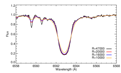
Figure 10: The impact of spectral resolution on the H_α line profile. The observed UVES spectrum of the star $19251846+0016550$ was taken from the Gaia-ESO archive.

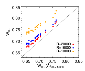
Figure 11: The comparison of the H_α width parameter measurements for different values of spectral resolving power.

In terms of galaxy formation, an interesting question is what is the fraction of observable stars in a typical L^∗ type galaxy that could be potentially studied with this technique. Fig. 12 shows the number of stars in our $T_{\!\mbox{\scriptsize\em\rm eff}}$-$\log{g}$ parameter space per $1000L_{\odot}$ in the Johnson-Cousins $V$ band, as a function of age (x-axis) and metallicity (colour coding). The plot was created using the population synthesis code underlying Schönrich & Bergemann (2014), and it represents a typical Galactic disc, calculated with the updated version (Schönrich & McMillan 2016) of the Schönrich & Binney (2009) model. The plot shows that all stellar populations with ages above $1$ Gyr are well-sampled at any metallicity, from the metal-rich $[\rm{Fe}/\rm{H}]+0.5$ to the most metal-poor $[\rm{Fe}/\rm{H}]-2.5$. The selection is up to an order of magnitude more efficient for metal-rich populations, because the cooler effective temperatures move larger parts of the giant branches into our $T_{\!\mbox{\scriptsize\em\rm eff}}$- $\log{g}$ parameter region. The gradient mostly reflects the radial metallicity gradient, with more stars being selected in the more metal-rich inner disc regions. This bias must be taken into account when comparing to galaxy models or when an unbiased dataset is constructed. Nevertheless, the selection probability is sufficiently large for all ages and metallicities, allowing to sample any population with age $\tau>1$ Gyr in units of $\geq 10^{5}$ solar masses.

To test for omitted variable biases in our empirical formula, we tested the residuals between masses derived from our method and the astroseismic values for trends with the stellar parameters $T_{\!\mbox{\scriptsize\em\rm eff}}$, $\log g$, $[\rm{Fe}/\rm{H}]$. This test confirmed that no significant trends could be found. I.e. our method does not have any significant bias with any stellar parameter, arguing against omitted variable biases and supporting the validity of the empirical formula.

To conclude, we have shown that our method samples well all stellar populations with ages above $1$ Gyr and still delivers sufficient sample sizes for moderate mass dwarf galaxies. Targeting bright giants, the method allows to obtain simultaneous age and chemical abundance (by applying the usual spectroscopic method of model atmospheres to the observed stellar spectrum) information far deeper than would be possible with asteroseismology of red giants, extending the possible survey volume to remote regions of the Milky Way and even to neighbouring galaxies like Andromeda or the Magellanic Clouds with present instrumentation on telescopes, like the VLT, Keck, or LBT. For example, with UVES/VLT or with the HIRES instrument at Keck (Vogt et al. 2011), optical high- or medium-resolution spectra can be acquired for stars with V magnitude $\sim 19$; in contrast the majority of red giants with asteroseismic ages from CoRoT or Kepler missions are brighter than $14$ mag (Mosser et al. 2010, Batalha et al. 2010, Hekker et al. 2011, Huber et al. 2014). In the future, our method opens a novel possibility to measure directly and consistently ages and chemical abundances of individual stars in more distant galaxies in the Local Group, e.g. with 4MOST, WEAVE, and E-ELT (Zerbi et al. 2014), which will reach stars with $V\sim 21$.

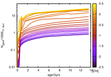
Figure 12: The number of red giant stars per $1000L_{\odot}$ in the Johnson-Cousins $V$ band, depending on age and metallicity (colour coding).

6 Summary and conclusions

We have analysed hydrogen (H_α) line profiles of $69$ red giant stars with high-resolution optical spectra obtained with different instruments. A part of the stellar spectra were acquired within the Gaia-ESO spectroscopic survey (Gilmore et al. 2012, Randich et al. 2013). For all these stars, asteroseismic data from CoRoT and Kepler observations are available, allowing us to compute their mass and age. We also include $73$ stars in $7$ open and globular clusters; their masses are derived from the CMD fitting. The sample covers a wide range range in metallicity, from metal-rich $+0.5$ to very metal-poor, $[\rm{Fe}/\rm{H}]<-2.5$, stars.

We find that the observed H_α profile presents a systematic dependence on fundamental stellar parameters. The profile of the unblended blue wing can be represented by a simple cubic-exponential function, which provides an excellent fit to the observed line profiles. The only parameters in the fit are the steepness, or width, of the H_α line and the minimum flux in the line core (Eq. 1). Both values appear to correlate with surface gravity and metallicity that suggests a more fundamental underlying relationship with the mass of a star. Indeed, there is a well-defined correlation between the steepness of H_α and stellar mass that can be described by a simple linear model (Eq. 2). This allows determination of masses with the accuracy 10-15% independent of stellar atmosphere and interior modelling. Although masses can be determined quite precisely with our method, it should be kept in mind that the estimates are slightly offset from the asteroseismic scale, such that at the low-mass end stellar masses are on average too high by $\sim 0.1$ M_⊙ and slightly lower at the high-mass end. This discrepancy could be caused by the asteroseismic mass estimates or by the second parameter problem of the H_α line. Still, the empirical masses can be used to determine ages of stars. The uncertainties of ages derived from the H_α line profile measurements are respectively $20-30$%, better than the classical stellar isochrone methods.

We cannot yet identify the physical mechanism underlying the relationship, because there are no stellar model atmospheres built from first principles that could be used to reproduce the observed H_α lines in red giants and explore their sensitivity to stellar mass. The standard 1D LTE models predict too weak H_α profiles compared to the observations. The more advanced 1D NLTE models with dynamics and winds are parametrised and do not explain the formation of the H_α lines, because they are designed to match the observed H_α profile shapes. 3D MHD chromospheric models have been computed for the Sun, but are not yet available for quantitative spectroscopy of stars with very different properties, like the RGB and RC stars. Having such models for a few red giants would be essential to understand the slope of the H_α-mass relation. Most likely, this would require global convection modelling and the inclusion of chromosphere. One other possibility is that stellar model atmospheres lack information about the stellar interior structure which, nevertheless, has an impact on the stellar atmosphere properties as recent work (Pinsonneault et al. 2014; Christensen-Dalsgaard et al. 2014) suggests. One interesting problem for the follow-up work would be to test the effect of variability in the H_α line on the $W_{H_{\alpha}}$ mass diagnostic. There is observational evidence (e.g. Cacciari et al. 2004, Meszaros et al. 2009 and references therein) that metal-poor stars ($[\rm{Fe}/\rm{H}]\lesssim-1.0$) more luminous than $\log(L/L_{\odot})\sim 2.5$ show time-dependent emission in the H_α wings, as well as asymmetries in the line core. There is currently no evidence for such processes in more metal-rich stars. Most red giants in our asteroseismic sample are fainter than this luminosity threshold and do not show emission or core shifts in the H_α line. With a large sample of stars for which spectra taken at different epochs are available it would be possible to test the effect of variability and possibly extend the method to very luminous red giants.

Our empirical results have interesting implications for spectroscopic observations of distant evolved stars: extremely metal-poor first stars, stars in the ’dark’ part of the Galaxy - the halo, in distant star clusters, Magellanic Clouds and in other galaxies of the Local Group, which will be routinely observable with new facilities like 4MOST and E-ELT. The instruments will reach targets as faint as V $\sim 21$ mag, that is $5$ times fainter compared to what is currently possible with asteroseismic methods, e.g. using Kepler or CoRoT mission data, and even with future missions like TESS. The observed optical spectra, in particular the conspicuous H_α line, may directly provide mass and age determinations for these stars, eliminating the need for model-dependent fitting methods based on stellar evolution and population synthesis models. We have also shown that our method, based on the spectral line H_α, samples well all stellar populations with ages above $1$ Gyr and still delivers sufficient sample sizes for moderate mass dwarf galaxies. Thus, the applications of our method are numerous, and extend our ability to measure the mass and age of stars to a much larger volume.

7 Appendix material

Table 3: Observational data for the Gaia-ESO stars.

CoRoT ID	Gaia-ESO ID	SNR	RAJ2000	DECJ2000	RV
			deg	deg	km$/$s
100922474	19251846+0016550	160	+291.3269167	+0.2819444	145
100974118	19253501+0022086	46	+291.3958750	+0.3690556	66
100864569	19250002+0026244	52	+291.2500833	+0.4401111	21
100856697	19245756+0052282	66	+291.2398333	+0.8745000	2
100853452	19245652+0031116	71	+291.2355000	+0.5198889	13
100597609	19232660+0127026	62	+290.8608333	+1.4507222	13
100821572	19244648+0119504	122	+291.1936667	+1.3306667	$-$38
100733870	19241853+0053232	54	+291.0772083	+0.8897778	11
101023768	19255284+0012484	222	+291.4701667	+0.2134444	51
100813799	19244402+0121257	134	+291.1834167	+1.3571389	59
100826123	19244789+0127475	43	+291.1995417	+1.4631944	57
100888944	19250775+0014218	17	+291.2822917	+0.2393889	$-$22
101080756	19261922+0023210	35	+291.5800833	+0.3891667	4
100761750	19242747+0045070	151	+291.1144583	+0.7519444	$-$160
100610961	19233129+0141224	58	+290.8803750	+1.6895556	85
100784327	19243467+0050077	119	+291.1444583	+0.8354722	14
100500736	19225173+0122202	31	+290.7155417	+1.3722778	13
101100065	19262648+0029588	77	+291.6103333	+0.4996667	22
101193334	19270157+0035230	44	+291.7565417	+0.5897222	18
100596299	19232616+0145326	21	+290.8590000	+1.7590556	50
101594554	19294723+0007019	39	+292.4467917	+0.1171944	40

Table 4: Stellar parameters and H_α  measurements for the Gaia-ESO field stars. Surface gravities are determined using the asteroseismic data.

CoRoT ID	Gaia-ESO ID	$W_{H_{\alpha}}$	$f_{0}$	age	error	mass	error	$T_{\!\mbox{\scriptsize\em\rm eff}}$	$\sigma$	$\log{g}$	$\sigma$	$[\rm{Fe}/\rm{H}]$	$\sigma$	$\log\frac{L}{L_{\rm Sun}}$
		Å	Å	Gyr		M⊙		K		dex		dex		dex
100922474	19251846+0016550	0.76	0.83	3.17	0.87	1.22	0.13	4957	23	2.39	0.01	-0.45	0.05	1.73
100974118	19253501+0022086	0.76	0.83	3.96	0.57	1.16	0.06	4933	58	2.51	0.01	-0.16	0.07	1.51
100864569	19250002+0026244	0.69	0.83	6.71	1.47	1.11	0.07	4772	52	2.77	0.01	-0.11	0.08	1.32
100856697	19245756+0052282	0.66	0.81	2.88	0.41	1.42	0.07	4681	134	2.56	0.01	0.18	0.12	1.64
100853452	19245652+0031116	0.71	0.82	7.03	0.99	0.97	0.06	4665	68	2.38	0.01	0.06	0.10	1.64
100597609	19232660+0127026	0.69	0.82	3.46	1.01	1.32	0.15	4638	62	2.47	0.02	0.11	0.03	1.74
100821572	19244648+0119504	0.68	0.81	13.31	1.60	0.92	0.03	4627	75	2.63	0.01	-0.12	0.04	1.39
100733870	19241853+0053232	0.67	0.80	5.80	3.33	1.10	0.10	4557	105	2.38	0.01	0.14	0.13	1.58
101023768	19255284+0012484	0.70	0.82	2.70	0.46	1.39	0.08	4765	57	2.52	0.01	-0.06	0.08	1.71
100813799	19244402+0121257	0.66	0.81	3.10	1.14	1.48	0.15	4638	79	2.72	0.01	0.14	0.08	1.65
100826123	19244789+0127475	0.68	0.81	2.60	0.81	1.49	0.16	4686	36	2.48	0.02	0.23	0.02	1.68
100888944	19250775+0014218	0.69	0.82	12.14	2.46	0.93	0.05	4949	181	2.58	0.01	-0.06	0.20	1.42
101080756	19261922+0023210	0.67	0.81	5.47	1.50	1.21	0.10	4658	43	2.66	0.01	-0.02	0.15	1.41
100761750	19242747+0045070	0.76	0.82	12.43	2.58	0.80	0.05	4792	58	2.15	0.02	-1.12	0.09	1.92
100610961	19233129+0141224	0.69	0.83	3.21	1.04	1.38	0.14	4790	36	2.71	0.02	-0.15	0.07	1.54
100784327	19243467+0050077	0.71	0.82	6.99	3.28	1.12	0.15	4167	87	1.79	0.02	-0.03	0.05	2.16
100500736	19225173+0122202	0.73	0.82	8.98	1.61	0.85	0.07	4802	49	2.39	0.01	-0.01	0.06	1.64
101100065	19262648+0029588	0.67	0.81	7.28	1.32	0.99	0.08	4520	45	2.42	0.01	0.23	0.07	1.59
101193334	19270157+0035230	0.70	0.83	6.02	1.60	1.19	0.09	4619	46	2.62	0.02	0.00	0.10	1.47
100596299	19232616+0145326	0.67	0.83	1.95	0.51	1.63	0.16	4684	42	2.56	0.02	0.07	0.11	1.76
101594554	19294723+0007019	0.68	0.83	4.04	0.90	1.27	0.08	4566	63	2.22	0.01	-0.20	0.09	1.87

Table 5: Observational data for the Gaia-ESO stars in clusters.

Cluster	Gaia-ESO ID	SNR	RAJ2000	DECJ2000	RV
			deg	deg	(km$/$s)
M67	08510838+1147121	163	+132.7849167	+11.7866944	33
M67	08513045+1148582	209	+132.8768750	+11.8161667	41
M67	08513577+1153347	191	+132.8990417	+11.8929722	34
M67	08514507+1147459	228	+132.9377917	+11.7960833	33
NGC1851	05133868-4007395	77	+78.4111667	$-$40.1276389	319
NGC1851	05134382-4001154	64	+78.4325833	$-$40.0209444	316
NGC1851	05134740-4004098	50	+78.4475000	$-$40.0693889	320
NGC1851	05135599-4004536	52	+78.4832917	$-$40.0815556	318
NGC1851	05135634-4003448	117	+78.4847500	$-$40.0624444	325
NGC1851	05135918-4002496	154	+78.4965833	$-$40.0471111	310
NGC1851	05135946-4005226	64	+78.4977500	$-$40.0896111	315
NGC1851	05135977-4002009	82	+78.4990417	$-$40.0335833	312
NGC1851	05140069-4003242	90	+78.5028750	$-$40.0567222	320
NGC1851	05140180-4002525	61	+78.5075000	$-$40.0479167	311
NGC1851	05140376-4001458	136	+78.5156667	$-$40.0293889	315
NGC1851	05141054-4003192	80	+78.5439167	$-$40.0553333	315
NGC1851	05141074-4004189	95	+78.5447500	$-$40.0719167	328
NGC1851	05141171-3959545	51	+78.5487917	$-$39.9984722	313
NGC1851	05141447-4001109	92	+78.5602917	$-$40.0196944	321
NGC1851	05141566-4000059	49	+78.5652500	$-$40.0016389	314
NGC1851	05141576-4003299	194	+78.5656667	$-$40.0583056	319
NGC1851	05141615-4001502	71	+78.5672917	$-$40.0306111	313
NGC1851	05141638-4003542	65	+78.5682500	$-$40.0650556	317
NGC1851	05141957-4004055	95	+78.5815417	$-$40.0681944	327
NGC1851	05141979-4006446	44	+78.5824583	$-$40.1123889	320
NGC1851	05142070-4004195	43	+78.5862500	$-$40.0720833	321
NGC1851	05142480-4002227	63	+78.6033333	$-$40.0396389	317
NGC1851	05142875-4003159	63	+78.6197917	$-$40.0544167	324
NGC1851	05142892-4004454	78	+78.6205000	$-$40.0792778	324
NGC1851	05135946-4005226	62	+78.4977500	$-$40.0896111	314
NGC1851	05140180-4002525	60	+78.5075000	$-$40.0479167	310
NGC1851	05141054-4003192	78	+78.5439167	$-$40.0553333	315
NGC1851	05142875-4003159	61	+78.6197917	$-$40.0544167	324
NGC2243	06292300-3117299	67	+97.3457917	$-$31.2916111	58
NGC2243	06292939-3115459	75	+97.3724583	$-$31.2627500	59
NGC2243	06294149-3114360	69	+97.4228750	$-$31.2433333	59
NGC2243	06294582-3115381	82	+97.4409167	$-$31.2605833	59
NGC2243	06290541-3117025	60	+97.2725417	$-$31.2840278	59
NGC2243	06290934-3110325	150	+97.2889167	$-$31.1756944	60
NGC2243	06291101-3120394	140	+97.2958750	$-$31.3442778	60
NGC2243	06292300-3117299	196	+97.3457917	$-$31.2916111	59
NGC2243	06292939-3115459	165	+97.3724583	$-$31.2627500	58
NGC2243	06293009-3116587	131	+97.3753750	$-$31.2829722	59
NGC2243	06293240-3117294	121	+97.3850000	$-$31.2915000	58
NGC2243	06293518-3117239	87	+97.3965833	$-$31.2899722	60
NGC2243	06294149-3114360	191	+97.4228750	$-$31.2433333	59
NGC2243	06294582-3115381	207	+97.4409167	$-$31.2605833	60
NGC2808	09110169-6451360	75	+137.7570417	$-$64.8600000	118
NGC2808	09112752-6451312	55	+137.8646667	$-$64.8586667	103
NGC2808	09115120-6448375	91	+137.9633333	$-$64.8104167	110
NGC2808	09121405-6448429	89	+138.0585417	$-$64.8119167	109
NGC2808	09122114-6447139	71	+138.0880833	$-$64.7871944	105
NGC2808	09123097-6456085	59	+138.1290417	$-$64.9356944	102
NGC2808	09123170-6449222	72	+138.1320833	$-$64.8228333	96
NGC2808	09123679-6451451	54	+138.1532917	$-$64.8625278	112
NGC2808	09123986-6455430	88	+138.1660833	$-$64.9286111	99
NGC2808	09124112-6446258	80	+138.1713333	$-$64.7738333	109
NGC2808	09124587-6453014	75	+138.1911250	$-$64.8837222	90
NGC2808	09125432-6445045	146	+138.2263333	$-$64.7512500	95
NGC2808	09115120-6448375	68	+137.9633333	$-$64.8104167	110
NGC2808	09120415-6450224	75	+138.0172917	$-$64.8395556	102
NGC2808	09123986-6455430	68	+138.1660833	$-$64.9286111	98
NGC6752	19103866-5954507	123	+287.6610833	$-$59.9140833	$-$27
NGC6752	19104208-6005293	133	+287.6753333	$-$60.0914722	$-$22
NGC6752	19114113-5959266	96	+287.9213750	$-$59.9907222	$-$32
NGC4372	12250660-7239224	92	186.5506	$-$72.67316	66
NGC4372	12253419-7235252	126	186.5506	$-$72.67316	70
NGC4372	12253882-7245095	77	186.5506	$-$72.67316	75
NGC4372	12264293-7241576	83	186.5506	$-$72.67316	69
NGC4372	12264875-7239413	80	186.5506	$-$72.67316	75
NGC5927	15272429-5037134	28	232.0144	-50.70945	$-$106
NGC5927	15275926-5039023	28	+231.9969167	$-$50.6506389	$-$103

Table 6: Stellar parameters and H_α measurements for the Gaia-ESO cluster stars. See Sect. 2.5 for more details.

Cluster	Gaia-ESO ID	$W_{H_{\alpha}}$	$f_{0}$	$T_{\!\mbox{\scriptsize\em\rm eff}}$	$\sigma$	$\log{g}$	$\sigma$	$[\rm{Fe}/\rm{H}]$	$\sigma$
		Å	Å	K		dex		dex
M67	08510838+1147121	0.66	0.81	4980	37	3.46	0.16	-0.05	0.07
M67	08513045+1148582	0.67	0.81	4939	50	3.47	0.08	0.05	0.09
M67	08513577+1153347	0.66	0.82	4964	25	3.46	0.10	-0.03	0.05
M67	08514507+1147459	0.67	0.82	4793	44	2.97	0.18	0.01	0.11
NGC1851	05133868-4007395	0.83	0.83	4375	24	1.12	0.36	-1.23	0.10
NGC1851	05134382-4001154	0.78	0.81	4871	55	2.00	0.05	-1.18	0.02
NGC1851	05134740-4004098	0.78	0.83	4892	51	2.36	0.01	-1.00	0.03
NGC1851	05135599-4004536	0.80	0.83	4837	24	2.17	0.14	-0.98	0.04
NGC1851	05135634-4003448	0.78	0.86	4291	34	0.99	0.38	-1.16	0.09
NGC1851	05135918-4002496	0.81	0.81	4917	35	1.55	0.04	-1.19	0.02
NGC1851	05135946-4005226	0.80	0.83	4539	111	1.66	0.16	-1.00	0.12
NGC1851	05135977-4002009	0.84	0.83	4509	6	1.42	0.13	-1.09	0.03
NGC1851	05140069-4003242	0.78	0.83	4536	5	1.23	0.17	-1.20	0.06
NGC1851	05140180-4002525	0.83	0.84	4562	90	1.63	0.21	-1.04	0.13
NGC1851	05140376-4001458	0.79	0.83	4619	35	1.83	0.07	-0.98	0.04
NGC1851	05141054-4003192	0.76	0.84	4412	47	1.39	0.08	-1.09	0.08
NGC1851	05141074-4004189	0.80	0.82	4372	19	1.14	0.26	-1.27	0.11
NGC1851	05141171-3959545	0.77	0.82	4938	9	2.20	0.31	-1.17	0.07
NGC1851	05141447-4001109	0.82	0.85	4317	6	1.21	0.57	-1.10	0.13
NGC1851	05141566-4000059	0.77	0.82	4947	28	2.15	0.03	-1.06	0.00
NGC1851	05141576-4003299	0.89	0.86	4366	36	1.21	0.33	-1.18	0.07
NGC1851	05141615-4001502	0.76	0.83	4880	37	2.22	0.09	-1.08	0.06
NGC1851	05141638-4003542	0.76	0.82	4761	50	1.99	0.15	-1.02	0.07
NGC1851	05141957-4004055	0.80	0.82	4394	9	1.12	0.22	-1.22	0.11
NGC1851	05141979-4006446	0.76	0.83	4993	48	2.38	0.19	-1.04	0.08
NGC1851	05142070-4004195	0.76	0.83	4949	98	2.38	0.15	-1.10	0.10
NGC1851	05142480-4002227	0.79	0.81	4712	160	1.73	0.49	-1.20	0.15
NGC1851	05142875-4003159	0.83	0.83	4600	6	1.59	0.12	-1.06	0.07
NGC1851	05142892-4004454	0.81	0.85	4443	17	1.50	0.07	-0.97	0.02
NGC1851	05135946-4005226	0.80	0.83	4539	111	1.66	0.16	-1.00	0.12
NGC1851	05140180-4002525	0.82	0.85	4562	90	1.63	0.21	-1.04	0.13
NGC1851	05141054-4003192	0.77	0.84	4412	47	1.39	0.08	-1.09	0.08
NGC1851	05142875-4003159	0.82	0.83	4600	6	1.59	0.12	-1.06	0.07
NGC2243	06292300-3117299	0.75	0.83	5039	43	2.63	0.11	-0.48	0.02
NGC2243	06292939-3115459	0.74	0.83	5031	28	2.54	0.16	-0.42	0.02
NGC2243	06294149-3114360	0.72	0.83	4788	48	2.60	0.26	-0.44	0.04
NGC2243	06294582-3115381	0.73	0.83	4962	55	2.39	0.14	-0.49	0.06
NGC2243	06290541-3117025	0.75	0.84	4961	24	2.52	0.11	-0.43	0.04
NGC2243	06290934-3110325	0.72	0.83	4910	36	2.72	0.10	-0.41	0.04
NGC2243	06291101-3120394	0.77	0.82	4895	30	2.46	0.18	-0.43	0.05
NGC2243	06292300-3117299	0.75	0.82	5039	43	2.63	0.11	-0.48	0.02
NGC2243	06292939-3115459	0.75	0.83	5031	28	2.54	0.16	-0.42	0.02
NGC2243	06293009-3116587	0.78	0.83	4689	49	2.15	0.39	-0.48	0.07
NGC2243	06293240-3117294	0.77	0.83	5028	47	2.57	0.13	-0.43	0.03
NGC2243	06293518-3117239	0.72	0.82	4980	35	2.89	0.08	-0.42	0.07
NGC2243	06294149-3114360	0.74	0.82	4788	48	2.60	0.26	-0.44	0.04
NGC2243	06294582-3115381	0.76	0.82	4962	55	2.39	0.14	-0.49	0.06
NGC2808	09110169-6451360	0.74	0.83	4356	59	1.28	0.26	-1.11	0.11
NGC2808	09112752-6451312	0.86	0.83	4709	19	1.66	0.24	-0.97	0.05
NGC2808	09115120-6448375	0.80	0.83	4292	29	1.27	0.07	-1.14	0.05
NGC2808	09121405-6448429	0.84	0.86	4423	41	1.27	0.25	-1.14	0.03
NGC2808	09122114-6447139	0.94	0.81	4520	8	1.49	0.10	-1.19	0.02
NGC2808	09123097-6456085	0.84	0.82	4598	8	1.72	0.04	-1.08	0.02
NGC2808	09123170-6449222	0.91	0.85	4384	34	1.27	0.30	-1.12	0.12
NGC2808	09123679-6451451	0.78	0.83	4710	40	1.71	0.15	-1.02	0.02
NGC2808	09123986-6455430	0.88	0.85	4316	62	1.22	0.30	-1.15	0.10
NGC2808	09124112-6446258	0.81	0.86	4358	52	1.25	0.19	-1.13	0.08
NGC2808	09124587-6453014	0.79	0.82	4417	38	1.39	0.09	-1.21	0.21
NGC2808	09125432-6445045	0.81	0.90	3872	36	0.78	0.25	-1.00	0.08
NGC2808	09115120-6448375	0.80	0.84	4292	29	1.27	0.07	-1.14	0.05
NGC2808	09120415-6450224	0.74	0.87	4207	62	1.01	0.22	-1.09	0.10
NGC2808	09123986-6455430	0.84	0.83	4316	62	1.22	0.30	-1.15	0.10
NGC6752	19103866-5954507	0.78	0.81	4845	62	1.80	0.10	-1.62	0.02
NGC6752	19104208-6005293	0.80	0.81	4736	59	1.65	0.26	-1.62	0.03
NGC6752	19114113-5959266	0.76	0.81	4966	21	1.98	0.11	-1.58	0.02
NGC4372	12250660-7239224	0.73	0.81	4669	41	1.41	0.43	-2.20	0.11
NGC4372	12253419-7235252	0.75	0.90	4414	100	1.09	0.50	-2.19	0.20
NGC4372	12253882-7245095	0.77	0.82	5101	442	2.00	0.83	-1.91	0.42
NGC4372	12264293-7241576	0.75	0.80	4698	21	1.42	0.15	-2.29	0.02
NGC4372	12264875-7239413	0.78	0.83	4639	23	0.93	0.21	-2.43	0.05
NGC5927	15272429-5037134	0.72	0.84	4796	83	2.44	0.25	-0.35	0.09
NGC5927	15275926-5039023	0.69	0.84	4411	98	2.21	0.12	-0.21	0.11

Table 7: Stellar parameters and H_α measurements for the Kepler stars from Thygesen et al. (2012). The stars marked with a star symbol are targets of Silva Aguirre et al. (2016, in preparation). Surface gravities are determined using the asteroseismic data.

Kepler ID	$W_{H_{\alpha}}$	$f_{0}$	age	error	mass	error	$T_{\!\mbox{\scriptsize\em\rm eff}}$	$\sigma$	$\log g$	$[\rm{Fe}/\rm{H}]$	$\sigma$		type
	Å	Å	Gyr		M⊙		K		dex	dex
2425631	0.69	0.83	2.79	1.19	1.46	0.19	4600	46	2.25	$-$0.04	0.05	1.96
2714397	0.70	0.82	4.05	1.37	1.09	0.11	5060	36	2.45	$-$0.59	0.28	1.79
3429205	0.65	0.81	3.52	0.98	1.33	0.10	5050	37	3.48	$-$0.11	0.10	0.85
3430868	0.73	0.83	8.84	1.86	1.01	0.06	5126	36	2.84	$-$0.06	0.07	1.39
3744043	0.64	0.81	4.62	0.51	1.19	0.03	4970	47	2.98	$-$0.31	0.09	1.27	RGB
3748691	0.69	0.83	4.35	1.75	1.31	0.14	4750	36	2.50	0.13	0.05	1.72	RGB
3955590	0.68	0.82	9.05	3.73	1.00	0.10	4645	36	2.23	$-$0.16	0.10	1.83
4072740	0.67	0.81	4.34	0.43	1.35	0.02	4805	53	3.37	0.23	0.15	0.88
4177025	0.70	0.83	10.40	3.73	0.90	0.15	4270	70	1.66	$-$0.24	0.06	2.21
4262505	0.68	0.83	3.43	1.10	1.33	0.12	4900	86	2.88	$-$0.20	0.06	1.40	RGB
4283484	0.82	0.83	5.71	0.72	0.93	0.05	5030	36	2.42	$-$0.77	0.05	1.75
4480358	0.77	0.84	8.45	3.78	0.90	0.12	4620	36	1.85	$-$0.96	0.11	2.16
4659706	0.64	0.80	2.15	0.87	1.70	0.21	4450	61	2.46	0.62	0.05	1.75
4671239∗	0.78	0.79	NaN	NaN	1.11	0.13	5000	100	2.40	$-$2.64	0.22	NaN
5113061	0.70	0.82	3.56	3.10	1.34	0.34	4190	36	1.54	0.01	0.06	2.47
5113910	0.72	0.84	6.06	3.34	1.03	0.14	4510	55	1.75	$-$0.31	0.05	2.27
5284127	0.67	0.81	6.31	0.61	1.07	0.04	4660	36	2.46	0.45	0.10	1.63	RC
5612549	0.77	0.84	6.71	0.80	0.92	0.05	4800	77	2.38	$-$0.33	0.05	1.70	RC
5701829	0.70	0.82	8.89	1.14	0.99	0.02	4880	59	3.08	$-$0.32	0.05	1.06
5779724	0.73	0.83	5.67	4.35	1.13	0.27	4240	36	1.68	$-$0.14	0.08	2.28
5859492	0.65	0.81	4.10	0.85	1.24	0.11	4800	36	2.49	0.19	0.09	1.72
5866965	0.72	0.85	8.66	4.27	0.92	0.15	4155	75	1.34	$-$0.52	0.09	2.49
6125893	0.69	0.82	3.64	3.00	1.39	0.37	4260	41	1.79	0.29	0.05	2.26
6547007	0.72	0.82	9.59	1.25	0.91	0.03	4785	36	2.50	$-$0.64	0.05	1.57
6579998	0.78	0.83	4.98	1.28	0.99	0.10	5070	36	2.45	$-$0.69	0.08	1.76	RC
6680734	0.73	0.82	6.33	2.18	1.07	0.10	4580	76	2.17	$-$0.38	0.05	1.90
6690139	0.68	0.82	2.64	0.30	1.45	0.03	5020	42	3.00	$-$0.13	0.05	1.35	RGB
6696436	0.72	0.83	7.54	1.22	1.04	0.04	4630	74	2.33	$-$0.26	0.09	1.74
6837256	0.73	0.83	2.92	0.35	1.30	0.04	4850	48	2.48	$-$0.65	0.05	1.77
7006979	0.70	0.82	4.64	0.61	1.10	0.05	4870	96	2.46	$-$0.19	0.25	1.72	RC
7340724	0.67	0.81	3.88	0.49	1.34	0.03	4879	112	3.05	0.04	0.10	1.22	RGB
7693833∗	0.78	0.79	4.10	0.42	1.09	0.04	4880	49	2.46	$-$2.23	0.06	1.72	RGB
7812552	0.68	0.82	7.47	0.77	0.99	0.02	5070	78	3.26	$-$0.59	0.05	0.95
8017159	0.74	0.82	5.26	4.11	0.99	0.25	4625	36	1.38	$-$1.95	0.05	2.67
8210100	0.70	0.82	3.15	1.00	1.37	0.14	4692	36	2.53	0.20	0.11	1.68	RC
8211551	0.73	0.82	10.32	0.92	0.77	0.03	4822	36	2.48	$-$0.20	0.06	1.53
8476245	0.78	0.81	4.29	1.10	1.09	0.09	4865	159	1.96	$-$1.28	0.22	2.22
8873797	0.69	0.81	7.50	1.28	0.98	0.07	4500	40	2.41	0.32	0.05	1.59	RC
9288026	0.76	0.83	7.19	3.02	0.88	0.17	5050	36	2.42	$-$0.36	0.05	1.73
9474021	0.69	0.85	3.99	4.23	1.18	0.37	4080	36	1.20	$-$0.47	0.05	2.71
10186608	0.69	0.83	5.95	1.82	1.02	0.13	4725	49	2.43	0.00	0.05	1.67	RC
10323222	0.68	0.82	4.83	0.59	1.27	0.03	4706	75	2.60	0.06	0.09	1.59	RGB
10403036	0.77	0.83	11.84	2.92	0.86	0.06	4505	87	1.92	$-$0.61	0.05	2.02
10404994	0.72	0.83	2.80	0.23	1.36	0.03	4855	42	2.54	$-$0.05	0.11	1.73	RC
11045542	0.72	0.84	4.66	3.08	1.14	0.21	4450	36	1.75	$-$0.51	0.09	2.29
11342694	0.67	0.80	8.27	3.01	1.15	0.11	4575	36	2.82	0.38	0.05	1.27
11444313	0.69	0.82	5.21	0.79	1.08	0.07	4750	36	2.46	$-$0.01	0.05	1.67	RC
11657684	0.75	0.83	5.51	1.63	1.04	0.13	4840	36	2.44	$-$0.09	0.07	1.71	RC

References

- Alfvén (1942) Alfvén, H. 1942, Nature, 150, 405
- Babcock (1961) Babcock, H. W. 1961, ApJ, 133, 572
- Bagnulo et al. (2003) Bagnulo, S., Jehin, E., Ledoux, C., et al. 2003, The Messenger, 114, 10
- Baker (2008) Baker 2008, Natl. Inst. Stand. Technol. Technical Note 1612, 8 pp
- Barklem et al. (2000) Barklem, P. S., Piskunov, N., & O’Mara, B. J. 2000, A&A, 355, L5
- Batalha et al. (2010) Batalha, N. M., Borucki, W. J., Koch, D. G., et al. 2010, ApJ, 713, L109
- Belkacem et al. (2011) Belkacem, K., Goupil, M. J., Dupret, M. A., et al. 2011, A&A, 530, A142
- Bergemann et al. (2012) Bergemann, M., Lind, K., Collet, R., Magic, Z., & Asplund, M. 2012, MNRAS, 427, 27
- Bergemann et al. (2014) Bergemann, M., Ruchti, G. R., Serenelli, A., et al. 2014, A&A, 565, A89
- Bruntt et al. (2012) Bruntt, H., Basu, S., Smalley, B., et al. 2012, MNRAS, 423, 122
- Cacciari et al. (2004) Cacciari, C., Bragaglia, A., Rossetti, E., et al. 2004, A&A, 413, 343
- Carlsson & Stein (2002) Carlsson, M., & Stein, R. F. 2002, ApJ, 572, 626
- Carlsson et al. (2007) Carlsson, M., Hansteen, V. H., de Pontieu, B., et al. 2007, PASJ, 59, 663
- Casagrande et al. (2014) Casagrande, L., Portinari, L., Glass, I. S., et al. 2014, MNRAS, 439, 2060
- Chaplin et al. (2014) Chaplin, W. J., Basu, S., Huber, D., et al. 2014, ApJS, 210, 1
- Christensen-Dalsgaard et al. (2014) Christensen-Dalsgaard, J., Silva Aguirre, V., Elsworth, Y., & Hekker, S. 2014, MNRAS, 445, 3685
- Coelho et al. (2015) Coelho, H. R., Chaplin, W. J., Basu, S., et al. 2015, MNRAS, 451, 3011
- Collet et al. (2011) Collet, R., Hayek, W., Asplund, M., et al. 2011, A&A, 528, A32
- D’Antona et al. (2016) D’Antona, F., Vesperini, E., D’Ercole, A., et al. 2016, MNRAS, 458, 2122
- De Angeli et al. (2005) De Angeli, F., Piotto, G., Cassisi, S., et al. 2005, AJ, 130, 116
- Dupree et al. (1984) Dupree, A. K., Hartmann, L., & Avrett, E. H. 1984, ApJ, 281, L37
- Dupree et al. (2009) Dupree, A. K., Smith, G. H., & Strader, J. 2009, AJ, 138, 1485
- Dupree et al. (2016) Dupree, A. K., Avrett, E. H., & Kurucz, R. L. 2016, ApJ, 821, L7
- Epstein et al. (2014) Epstein, C. R., Elsworth, Y. P., Johnson, J. A., et al. 2014, ApJ, 785, L28
- Fontenla et al. (2009) Fontenla, J. M., Curdt, W., Haberreiter, M., Harder, J., & Tian, H. 2009, ApJ, 707, 482
- García et al. (2014) García, R. A., Ceillier, T., Salabert, D., et al. 2014, A&A, 572, A34
- Ghezzi & Johnson (2015) Ghezzi, L., & Johnson, J. A. 2015, ApJ, 812, 96
- Gilmore et al. (2012) Gilmore, G., Randich, S., Asplund, M., et al. 2012, The Messenger, 147, 25
- Gudiksen et al. (2011) Gudiksen, B. V., Carlsson, M., Hansteen, V. H., et al. 2011, A&A, 531, A154
- Gustafsson et al. (2008) Gustafsson, B., Edvardsson, B., Eriksson, K., et al. 2008, A&A, 486, 951
- Hansteen (2004) Hansteen, V. H. 2004, Multi-Wavelength Investigations of Solar Activity, 223, 385
- Hansteen et al. (2015) Hansteen, V., Guerreiro, N., De Pontieu, B., & Carlsson, M. 2015, ApJ, 811, 106
- Hartmann & MacGregor (1980) Hartmann, L., & MacGregor, K. B. 1980, ApJ, 242, 260
- Hekker et al. (2011) Hekker, S., Gilliland, R. L., Elsworth, Y., et al. 2011, MNRAS, 414, 2594
- Huber et al. (2014) Huber, D., Silva Aguirre, V., Matthews, J. M., et al. 2014, ApJS, 211, 2
- Jørgensen & Lindegren (2005) Jørgensen, B. R., & Lindegren, L. 2005, A&A, 436, 127
- Kurucz (1979) Kurucz, R. L. 1979, ApJS, 40, 1
- Leenaarts (2010) Leenaarts, J. 2010, Mem. Soc. Astron. Italiana, 81, 576
- Leenaarts et al. (2012) Leenaarts, J., Carlsson, M., & Rouppe van der Voort, L. 2012, ApJ, 749, 136
- Leenaarts et al. (2015) Leenaarts, J., Carlsson, M., & Rouppe van der Voort, L. 2015, ApJ, 802, 136
- Magic et al. (2013) Magic, Z., Collet, R., Asplund, M., et al. 2013, A&A, 557, A26
- Magic et al. (2013) Magic, Z., Collet, R., Hayek, W., & Asplund, M. 2013, A&A, 560, A8
- Martig et al. (2016) Martig, M., Fouesneau, M., Rix, H.-W., et al. 2016, MNRAS, 456, 3655
- Mashonkina et al. (2008) Mashonkina, L., Zhao, G., Gehren, T., et al. 2008, A&A, 478, 529
- Masseron & Gilmore (2015) Masseron, T., & Gilmore, G. 2015, MNRAS, 453, 1855
- Meibom et al. (2015) Meibom, S., Barnes, S. A., Platais, I., et al. 2015, Nature, 517, 589
- Meszaros et al. (2009) Meszaros, S., Avrett, E., & Dupree, A. K. 2009, AJ, 138, 615
- Miglio et al. (2012) Miglio, A., Brogaard, K., Stello, D., et al. 2012, MNRAS, 419, 2077
- Mosser et al. (2010) Mosser, B., Belkacem, K., Goupil, M.-J., et al. 2010, A&A, 517, A22
- Ness et al. (2015) Ness, M., Hogg, D. W., Rix, H., et al. 2015, arXiv:1511.08204
- Pinsonneault et al. (2014) Pinsonneault, M. H., Elsworth, Y., Epstein, C., et al. 2014, ApJS, 215, 19
- Pont & Eyer (2004) Pont, F., & Eyer, L. 2004, MNRAS, 351, 487
- Przybilla & Butler (2004) Przybilla, N., & Butler, K. 2004, ApJ, 610, L61
- Randich et al. (2013) Randich, S., Gilmore, G., & Gaia-ESO Consortium 2013, The Messenger, 154, 47
- Rutten (2008) Rutten, R. J. 2008, First Results From Hinode, 397, 54
- Schönrich & Binney (2009) Schönrich, R., & Binney, J. 2009, MNRAS, 396, 203