Measuring protoplanetary disk gas surface density profiles with ALMA

Abstract

The gas and dust are spatially segregated in protoplanetary disks due to the vertical settling and radial drift of large grains. A fuller accounting of the mass content and distribution in disks therefore requires spectral line observations. We extend the modeling approach presented in Williams & Best (2014) to show that gas surface density profiles can be measured from high fidelity ¹³CO integrated intensity images. We demonstrate the methodology by fitting ALMA observations of the HD 163296 disk to determine a gas mass, $M_{\rm gas}=0.048\,M_{\odot}$, and accretion disk characteristic size $R_{c}=213$ au and gradient $\gamma=0.39$. The same parameters match the C¹⁸O 2–1 image and indicates an abundance ratio [¹³CO]/[C¹⁸O] of 700 independent of radius. To test how well this methodology can be applied to future line surveys of smaller, lower mass T Tauri disks, we create a large ¹³CO 2–1 image library and fit simulated data. For disks with gas masses $3-10\,M_{\rm Jup}$ at 150 pc, ALMA observations with a resolution of $0\farcs 2-0\farcs 3$ and integration times of $\sim 20$ minutes allow reliable estimates of $R_{c}$ to within about 10 au and $\gamma$ to within about 0.2. Economic gas imaging surveys are therefore feasible and offer the opportunity to open up a new dimension for studying disk structure and its evolution toward planet formation.

1 Introduction

The gas and dust in circumstellar disks share a common origin in the interstellar medium but rapidly evolve to a very different states. The high densities, cool temperatures, and low turbulence in disks provide the ideal conditions for the growth of dust grains to millimeter sizes and beyond. As the ratio of surface area to mass decreases, the grains feel a headwind from the slightly sub-Keplerian motion of the viscous gas and they drift inwards while also sedimenting toward the midplane. A wealth of fascinating physical processes can then occur in this two-fluid medium that are not found in other astronomical environments and that typically end with a planetary system (Armitage, 2013).

Protoplanetary disks radiate most strongly in the infrared and measurements of excess emission above the photosphere at these wavelengths is the most sensitive way to diagnose the presence of dust around stars. The emission at millimeter wavelengths is much weaker but the continuum is generally optically thin and therefore provides a more precise way to measure the amount and, through interferometry, the distribution of the dust (Williams & Cieza, 2011).

Molecular gas, though by far the dominant constituent by mass, is actually much harder to observe since the gas is too cool for H₂ to emit significantly. As with observations of molecular clouds and cores, the gas is most readily detected through millimeter observations of rotational transitions of CO and other trace molecules that lie within a warm molecular layer (Aikawa et al., 2002). The high optical depth of the infrared continuum obscures line emission which is otherwise seen in the inner regions of transition disks with dust-depleted holes (Pontoppidan et al., 2008). The dust becomes transparent at millimeter wavelengths and many rotational lines can in principle be detected. The ¹²CO lines are optically thick, however, and most useful as a diagnostic of the temperature and kinematics of the gas than of its mass (Beckwith & Sargent, 1993).

Williams & Best (2014, hereafter Paper I) showed the utility of CO isotopologue observations for measuring disk gas masses independently from that of the dust. The intensity of these rarer species, with their lower optical depths, depends primarily on the amount of the gas and secondarily on its temperature and density. Freeze-out in the cold midplane and photo-dissociation in the upper disk atmosphere must also be taken into account but we found that most of the gas in typical disks resides in the molecular layer between these two regions. We concluded that the combination of spatially and velocity integrated ¹³CO and C¹⁸O line luminosities constrains disk gas masses to a factor of about 3–10, a result that has recently been confirmed in a much larger Atacama Large Millimeter/Submillimeter Array (ALMA) survey of Lupus disks by Ansdell et al. (2016). This moderate level of precision is sufficient to show that the bulk gas-to-dust ratios in most protoplanetary disks are different than the interstellar medium value of 100, a key finding that may help explain why the abundant super-Earths and Neptunes in exoplanet surveys avoided runaway growth to Jupiters (Helled & Bodenheimer, 2014).

In this paper, we examine whether we can extend the modeling methodology in Paper I and use CO isotopologue maps to determine the distribution of the gas. Techniques to determine dust surface density profiles from resolved continuum images are now well established (e.g., Lay et al., 1997; Andrews & Williams, 2007). As the dust and gas are spatially decoupled, however, we cannot simply extrapolate this to the gas distribution (Panić et al., 2009). ALMA will make resolved disk images of CO isotopologues routine and there is a need to develop simple modeling tools that can quickly and reliably derive basic disk gas properties in a uniform way to allow comparative studies in large surveys. Our focus here is on observations of ¹³CO as it is strong enough to survey and is more dependent on the surface density of the gas than its temperature. §2 describes the modeling procedure, the creation of an image library, and an interpolation routine that allows a continuous sampling of parameter space necessary for error estimation. We then fit observations of the HD 163296 disk as a proof-of-concept. In the following section, §3, we create a generic grid of models more suitable for lower mass disks around lower mass, T Tauri stars. By comparing simulated images to gaussian fits and the rest of the image library, we find that that ALMA integrations of a few to a few tens of minutes (depending on gas mass) at $\sim 0\farcs 2-0\farcs 3$ resolution should reveal the gas surface density profiles of typical disks in nearby star-forming regions. We summarize these results and discuss their implications in §4.

2 The HD 163296 disk

Protoplanetary disks are generally compact with weak line emission. Consequently, there are only a few disks with well resolved, high signal-to-noise ¹³CO maps in the literature. The exceptional disk around the nearby (122 pc) Herbig Ae star HD 163296 is, fortunately, both big and bright. Moreover, early ALMA observations of ¹³CO and other lines are publicly available through its Science Verification program and it has been modeled independently by two groups (Rosenfeld et al., 2013; de Gregorio-Monsalvo et al., 2013). It is therefore an ideal source to demonstrate the feasibility of our procedure.

2.1 Description of the model

We follow the methodology in Paper I but create a library of resolved images rather than a table of total line luminosities. The gas is assumed to be azimuthally symmetric, in hydrostatic equilibrium and under Keplerian rotation. Nominally, there are nine free parameters but we are able to considerably reduce these based on previous studies. In particular, we set the stellar mass, $2.3\,M_{\odot}$, and inclination, $i=45^{\circ}$, based on Qi et al. (2011) and we use the gas temperature structure, $T_{\rm gas}(R,Z)$, described in Rosenfeld et al. (2013). This leaves just three remaining parameters, $M_{\rm gas}$, $R_{c}$, and $\gamma$, that determine the accretion disk gas surface density distribution (Lynden-Bell & Pringle, 1974),

$$\Sigma_{\rm gas}(R)=(2-\gamma)\,\frac{M_{\rm gas}}{2\pi R_{c}^{2}}\left(\frac{R}{R_{c}}\right)^{-\gamma}\,\exp\left[-\left(\frac{R}{R_{c}}\right)^{2-\gamma}\right].$$ (1)

Having specified the density and temperature structure, we define the warm molecular layer where CO is in the gas phase and can emit with a lower boundary set by a freeze-out temperature of 20 K and an upper boundary set by dissociation at column densities $N_{\rm H_{2}}>N_{\rm dissoc}=1.3\times 10^{21}\,{\rm H}_{2}$ cm^-2. Within this region, we assume a constant CO abundance $\rm{[\mbox{${}^{12}$CO}]/[H_{2}]}=1\times 10^{-4}$ and isotopologue ratio, [¹²CO]/[¹³CO]=70.

We then calculate the ¹³CO 2–1 line emission using the radiative transfer code RADMC-3D. The output is a spectral line datacube with a resolution of 5 AU and 0.1 ${\rm km~{}s^{-1}}$. The ordered motion of a Keplerian disk means that different regions of a disk generally have different radial velocities. As a result, we found that it is not necessary to make tomographic comparisons of channel maps to discriminate between models and that velocity integrated (zero-moment) maps suffice. This reduces the computational requirements of memory, disk space, and speed considerably. Finally, we compared models with LTE and NLTE excitation and found no substantial difference ($<1$ mJy ${\rm km~{}s^{-1}}$ pixel^-1).

2.2 Image interpolation

We created an image library by running 748 models over the range of parameters shown in Table 1. It is straightforward to determine the best fit model parameters by minimizing the squared difference between the image library to the data. This simple chi-squared analysis does not allow us to determine parameter errors, however, as the model is non-linear (Andrae et al., 2010). A more statistically robust approach is to sample the parameter space using a Markov Chain Monte Carlo (MCMC) technique. The radiative transfer calculation takes several minutes to run for each set of disk parameters and is too slow to carry out the required $\gg 10^{4}$ model calculations directly, however, and we therefore designed a simple routine to interpolate images within the model grid.

Table 1: Parameter range of the HD 163296 grid

Parameter	Range	Step	Units
$M_{\rm gas}$	4.0–5.5	0.5	$10^{-2}\,M_{\odot}$
$R_{c}$	160–320	10	au
$\gamma$	0.0–1.0	0.1
inclination	45	$\cdots$	∘

We wish to determine the image $I({\bf p})$ at a set of parameter values ${\bf p}=\{p_{i};\ i=0,1,...,N\}$. For each index $i$, we bound the parameter by grid points, $g_{i}^{0}\leq p_{i}\leq g_{i}^{1}$. There are $2^{N}$ vertices of the $N$-dimensional cube defined by these grid points, ${\bf v}=\{g_{i}^{j};\ i=0,1,...,N\}$ over all combinations $j=0,1$. We then linearly interpolate the image library,

$$I({\bf p})=\sum_{\bf v}w({\bf v})I({\bf v}),$$ (2)

where the weights at each vertex,

$$w({\bf v})=\prod_{i}\left(1-\frac{|p_{i}-v_{i}|}{g_{i}^{1}-g_{i}^{0}}\right).$$ (3)

This procedure is fast and can be readily modified to allow different weighting schemes or to extend over a wider parameter space beyond the bounding grid points. It sufficed for our purposes where we found that interpolated images averaged within 3% of a full radiative transfer calculation. This efficient method to calculate model images over a continuous range of parameter values now permits an MCMC analysis.

2.3 Parameter estimation

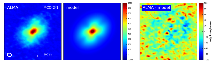
Figure 2: Comparison of ¹³CO integrated intensity images. The left panel shows the ALMA Science Verification map, the central panel the model fit for the median of MCMC model parameters, and the right panel shows the difference image. The colorbars show the range of intensities for each map; the ALMA and model images on the same scale from $-100$ to 1000 mJy ${\rm km~{}s^{-1}}$ beam^-1, and the difference image from $-100$ to 100 mJy ${\rm km~{}s^{-1}}$ beam^-1.

The MCMC modeling was run with a flat prior for each parameter over the range shown in Table 1 using the emcee software package (Foreman-Mackey et al., 2013). The projection of the 3-dimensional parameter space is shown in Figure 2, from which we calculate median and 68% ($\pm 1\sigma$) confidence intervals, $M_{\rm gas}=0.048^{+0.003}_{-0.003}\,M_{\odot},R_{c}=213^{+7}_{-7}\,{\rm AU},\gamma=0.39^{+0.09}_{-0.08}$. The inferred gas mass agrees well with that derived from the comparison of ¹³CO – C¹⁸O luminosities in Paper I ($0.047\,M_{\odot}$). The apparently high precision obtained here reflects the rigidity of the temperature structure imposed in our models, which we discuss further in §4.

The data, median fit, and difference image are shown in Figure 1. Given the simplicity of the model, the overall fit is good with peak residuals less than 10% of the image maximum and consistent with a gaussian with standard deviation 27 mJy ${\rm km~{}s^{-1}}$, comparable to the rms noise level of the data. Due to the separation in sky position with velocity, the channel maps (not shown here) are correspondingly well fit.

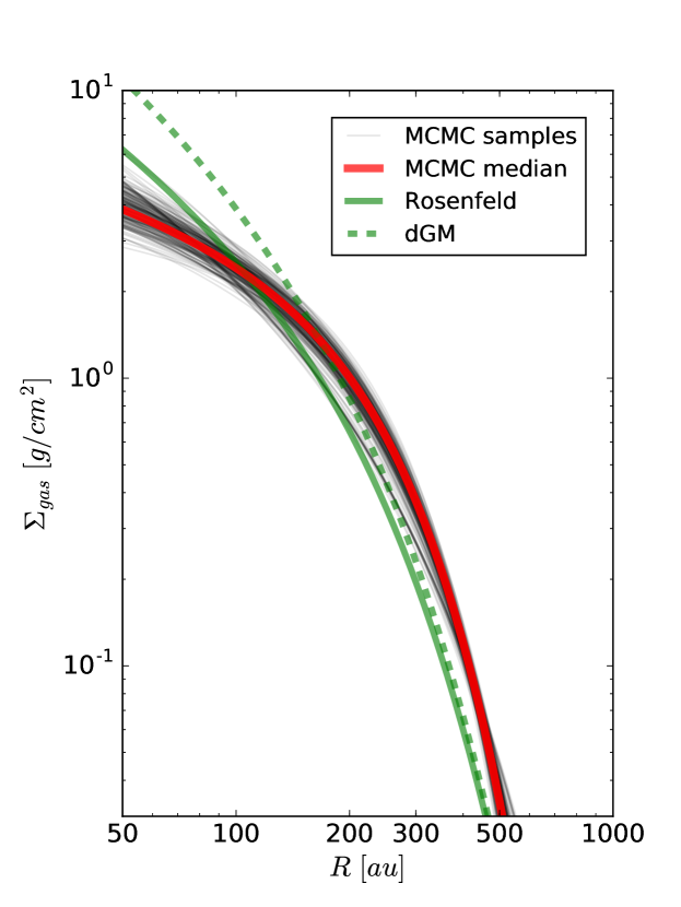
Figure 3: Gas surface density profiles derived from fitting the the HD 163296 ¹³CO 2–1 integrated map. 200 samples from the $5\times 10^{4}$ MCMC samples are shown in gray to illustrate the range probed by the random walk. The profile for the median parameter values is shown in red. For comparison, the profiles derived from fitting the ¹²CO 3-2 channel maps by (Rosenfeld et al., 2013; de Gregorio-Monsalvo et al., 2013) are shown in green. The differences, which are due to the higher optical depth of the ¹²CO line and the nature of the fits, are discussed further in the text.

The inferred surface density density profiles, $\Sigma_{\rm gas}(R)$, are shown in Figure 3. For comparison, we also plot the surface density profiles that were determined from fitting the ¹²CO 3-2 data by Rosenfeld et al. (2013) (after normalizing to the same [CO]/[H₂] abundance) and de Gregorio-Monsalvo et al. (2013). Both find higher central densities, steeper profiles, and smaller outer disk radii than our fits to ¹³CO. This cannot be due to higher optical depth in the ¹²CO line nor to selective photo-dissociation of ¹³CO in the outer parts of the disk, both of which would produce the opposite effect seen here, i.e., a larger CO and smaller ¹³CO disk. More likely, it simply reflects the uncertainties inherent in modeling a single line.

2.4 Comparison with the C¹⁸O image

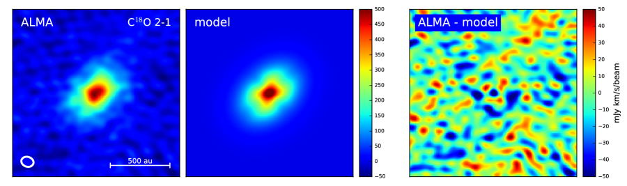
Figure 4: Comparison of C¹⁸O integrated intensity images. The left panel shows the ALMA Science Verification map, the central panel the model fit for the disk parameter values derived from the ¹³CO fitting, and the right panel shows the difference image. The colorbars show the range of intensities for each map; the ALMA and model images on the same scale from $-50$ to 500 mJy ${\rm km~{}s^{-1}}$ beam^-1, and the difference image from $-50$ to 50 mJy ${\rm km~{}s^{-1}}$ beam^-1.

The ALMA Science Verification data for HD 163296 also include the C¹⁸O 2–1 line which, being of lower optical depth than the same ¹³CO transition, allows a further test of the model. We ran the RADMC-3D radiative transfer for this C¹⁸O line with the median surface density parameters derived above and only varied the [CO]/[C¹⁸O] abundance to minimize the least squares difference with the zero-moment map. The data, image, and difference in Figure 4. The fit is very good with peak residuals at about 10% of the image maximum. The inferred abundance ratio is [CO]/[C¹⁸O]=700 and there are no obvious systematics in the difference image suggesting that the abundance does not greatly vary with disk radius.

As a rare isotopologue, C¹⁸O cannot self-shield as effectively as CO and is expected to be selectively photo-dissociated (van Dishoeck & Black, 1988). Indeed the comparison of ¹³CO and C¹⁸O line luminosities in Paper I showed evidence for this in Taurus disks. Detailed thermo-chemical models confirm that this can have a significant impact on the C¹⁸O emission from low-mass disks though not for such massive disks as HD 163296 (Miotello et al., 2014). Future observations of T Tauri disks can examine this important effect and assess whether it may explain the variation of oxygen isotopes in the Solar System (McKeegan et al., 2011).

3 T Tauri model grid

3.1 Description

Most stars are lower mass than HD 163296 and their dust disks tend to be considerably smaller in both mass and size (Andrews et al., 2010). Paper I and Ansdell et al. (2016) show that the median Class II disk gas mass in Taurus and Lupus is small, $\sim 1\,M_{\rm Jup}=10^{-3}\,M_{\odot}$, and that Minimum Mass Solar Nebula (MMSN) disks with masses $\sim 10^{-2}\,M_{\odot}$ are rare. Whereas most studies of disk structure to date have naturally tended toward observations of bright (i.e., massive) and large disks, recent work shows that some low-mass disks may be very small, at least as measured in the continuum (Piétu et al., 2014). Nevertheless, the ALMA Science Verification data of HD 163926 analyzed in §2 had, by today’s standards, low resolution and high noise. If we scale by the dynamic range in spatial and intensity scales, $\sim 10$ and 40 respectively, it seems feasible that current and future ALMA observations should be able to map the intensity profile of these lower mass disks with sufficient fidelity to derive their gas surface densities.

To be more quantitative and assess the best combination of resolution and noise level to measure gas profiles, we defined a generic model grid based on the parameters of disks around T Tauri stars. As with HD 163296, we fix the stellar mass and temperature structure under the expectation that they can be determined through fitting ¹²CO observations. Following the nomenclature in Paper I, their values are set to

$$M_{\rm star}=0.5\,M_{\odot},~{}T_{\rm mid,1}=100\,{\rm K},~{}T_{\rm atm,1}=500\,{\rm K},~{}q=0.5.$$ (4)

¹²CO kinematics, or even the continuum image, will also provide a good measure of the disk inclination to the line of sight. As the inclination changes the image surface brightness, however, it affects our ability to measure gas surface density profiles and we therefore consider a range of values in the grid. The set of surface density parameters and inclination are listed in Table 2. For comparison with planned and ongoing ALMA surveys, we created zero-moment maps of the ¹³CO 2–1 line for a distance of 150 pc and a pixel scale of 5 au ($0\farcs 03$).

Table 2: Parameter values of the T Tauri grid

Parameter	Range	Step	Units
$M_{\rm gas}$	0.1–3.0	0.1	$10^{-2}\,M_{\odot}$
$R_{c}$	20–200	20	au
$\gamma$	0.0–1.0	0.1
inclination	30–60	15	∘

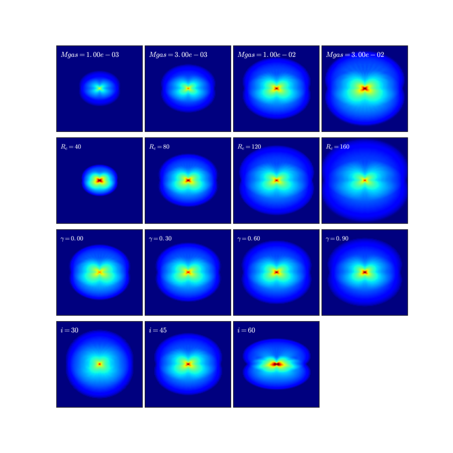
Figure 5: Montage of ¹³CO 2–1 integrated intensity maps from the T Tauri disk model library. Each row shows the effect of varying a single parameter, whose value is shown in the upper left of each subplot. Unless otherwise labeled, the default values are $M_{\rm gas}=10^{-2}\,M_{\odot},R_{c}=100\,{\rm au},\gamma=0.5,i=45^{\circ}$. The images are shown with square-root scaling varying from 0 to 100 mJy per 5 AU$\times$5 AU cell size.

The resulting image library consists of 9900 models. Figure 5 shows the effect of varying the three surface density parameters and inclination. $M_{\rm gas}$ scales the intensity at each pixel, though not perfectly linearly or uniformly across an image due to opacity. Disks with small $R_{c}$ are compact with a high central brightness whereas the largest disks have low surface brightness. The center also brightens as the density gradient $\gamma$ increases. The bottom row shows the strong effect of inclination on the disk aspect ratio and brightness distribution. We assume this to be fixed in deriving the three other parameters but allow for its variation when considering the statistical accuracy of a survey.

3.2 Criteria for distinguishing a disk from a gaussian

The gas surface density parameters each have a different effect on the ¹³CO zero-moment map and each can, in principle, be distinguished from one another. As observations are inherently noisy and of finite resolution, however, the determination of parameters will not be exact and may be biased. We can assess the effects of parameter variation, at least within the limitations of our model framework, by convolving the images and adding gaussian random noise.

ALMA can now readily achieve a resolution from $\ll 0\farcs 1$ to about an arcsecond at the 220 GHz frequency of ¹³CO 2–1. Independent of the array configuration, the noise per beam for a given frequency depends only on the integration time but as the flux per beam decreases with increasing resolution for a resolved source, there is a tradeoff between spatial and intensity dynamic range. Based on the model disk sizes and line fluxes, we consider a range of (circular) beamsizes from $0\farcs 1$ to $0\farcs 4$ FWHM, and rms noise levels from 1 to 30 mJy beam^-1 ${\rm km~{}s^{-1}}$. As a guide to the array integration time, the ALMA sensitivity calculator, shows that an rms of $\sigma=10$ mJy ${\rm km~{}s^{-1}}$ beam^-1 at 220 GHz can be achieved in 2 minute integrations at $-30^{\circ}$ declination.

Before comparing a simulated image against the model library, it is important to test the ansatz that the image can be distinguished as a disk and not a simpler gaussian description. We fit an elliptical gaussian to a simulated image and calculate the flux distribution of the residuals. A Kolomogorov-Smirnov test of the goodness of fit of a gaussian to the residual flux distribution then shows how well the image can be distinguished from the elliptical gaussian fit.

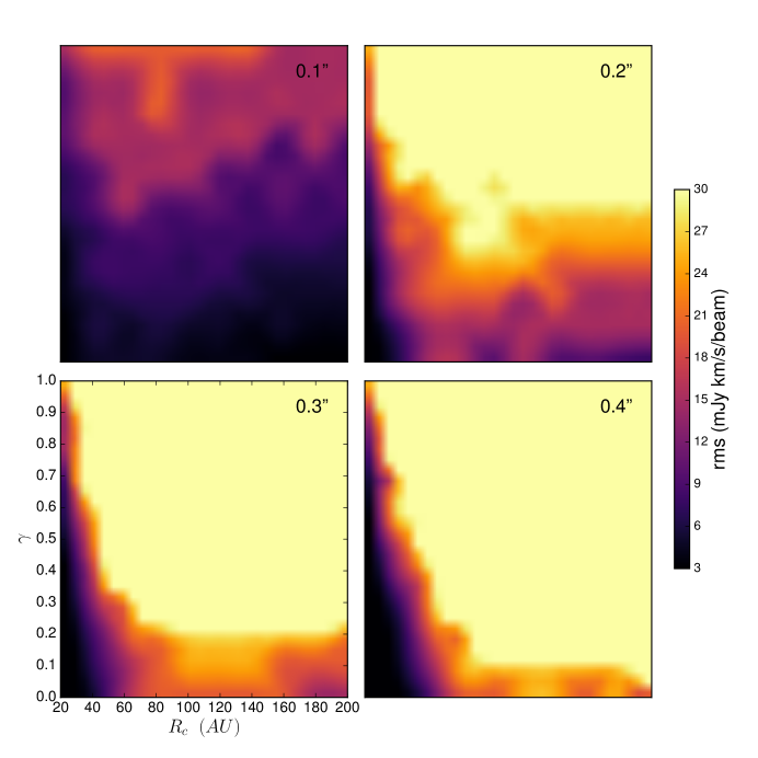
Figure 6: Plots of the rms noise level required to distinguish a T Tauri ¹³CO 2–1 disk model with $M_{\rm gas}=10^{-2}\,M_{\odot}$ from an elliptical gaussian fit. Each plot is shown as a function of $R_{c}$ and $\gamma$ and the different panels have different beam sizes, as labeled in the upper right corner. Large disks and steep profiles are readily distinguished from a gaussian at moderate resolution, $0\farcs 3-4$, but small and/or flatter disks require higher resolution and low rms.

For each convolved disk model, we increase the rms noise until a gaussian fit is sufficient. This noise level is plotted for the four different beam sizes and MMSN disks ($M_{\rm gas}=10^{-2}\,M_{\odot}$) as a function of $R_{c}$ and $\gamma$ in Figure 6. The bright yellow regions show where disks are readily distinguished as disk-like even in shallow integrations with relatively high noise levels, 30 mJy ${\rm km~{}s^{-1}}$ beam^-1. There is a balance between resolution and signal-to-noise. A smaller beamsize provides more independent measurements of the disk shape and is necessary to resolve compact disks, but there is less flux per beam. The smallest beamsize shown here, $0\farcs 1$, is so fine that very sensitive observations are necessary to image the gas structure. For larger beamsizes, the purple regions indicate that an rms of 10 mJy ${\rm km~{}s^{-1}}$ beam^-1 can distinguish all but the smallest disks, $R_{c}\lesssim 40$ au, with flat profiles, $\gamma\lesssim 0.5$. Not surprisingly, this unresolved region is larger for the largest beam size, $0\farcs 4$.

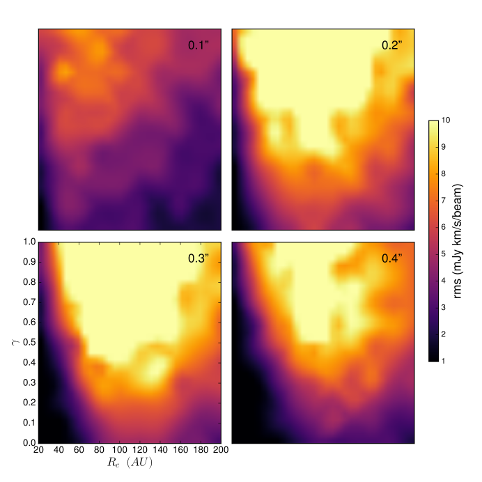
Figure 7: Similar plot as Figure 6 but for a Jupiter mass disk, $M_{\rm gas}=10^{-3}\,M_{\odot}$. Note the change in color scale for the rms. Due to the much lower flux levels, large disks are hard to distinguish from a gaussian even at the largest beam size here, $0\farcs 4$, and the optimum range is an intermediate resolution, $0\farcs 2-3$. Even then, low noise levels are required to study these low mass disks.

The fainter, lower mass disks require more sensitive observations. Figure 7 shows the same calculation as above for but a Jupiter mass disk, $M_{\rm gas}=10^{-3}\,M_{\odot}$, and a color scale scaled lower by a factor of three. As before, the signal-to-noise level in a $0\farcs 1$ beam is too low to study the gas structure, and small/flat disks are inaccessible to all but the most sensitive observations. However, unlike the MMSN disks, large and flat disks $R_{c}\gtrsim 160$ au, $\gamma\lesssim 0.3$ are also hard to study due to their low, extended surface brightness. For these low mass disks, an intermediate sized beam, $0\farcs 2-0\farcs 3$ and low noise levels, $\sim 3$ mJy ${\rm km~{}s^{-1}}$ beam^-1 ($\sim 20$ minute integrations) are optimal.

3.3 Accuracy of parameter estimation

If we can observe a disk with sufficient resolution and sensitivity to differentiate it from a gaussian, the next question is how well can we determine the gas surface density profile. We use the same image interpolation scheme described in §2.2 to continuously sample the parameter space and find the best fit to a given simulated image using the python scipy.optimize routine. We do not estimate errors in this case but rely on the statistics of the model comparisons to assess the accuracy to which we can measure each parameter.

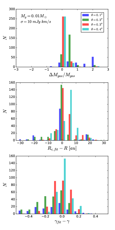
Figure 8: The precision with which the gas surface density profile of a disk can be measured, color-coded by resolution. The model disks have a gas mass, $M_{\rm gas}=10^{-2}\,M_{\odot}$, and the noise in the simulated observations is 10 mJy ${\rm km~{}s^{-1}}$ beam^-1. The top panel shows the fractional precision to which we recover the input gas mass. The two lower panels show the absolute difference between the input and best fit $R_{c}$ and $\gamma$. As only those disks which can be distinguished from a gaussian are shown, there are fewer models at the $\theta_{\rm FWHM}=0\farcs 1$ beam size (see Figure 6).

Figure 8 plots histograms of the difference between the input and fitted parameters for all disks with mass $M_{\rm gas}=10^{-2}\,M_{\odot}$, observed with an rms noise level of 10 mJy ${\rm km~{}s^{-1}}$ beam^-1. The histograms are color-coded by beam size and only those disks that can be distinguished from a gaussian are shown. Hence there are fewer disks in the dark blue ($\theta_{\rm FWHM}=0\farcs 1$). The top panel shows the relative difference between the fitted gas mass and the input value. In general the mass is measured from the profile fitting alone to within about 50% for all but the noisy, high resolution images. The two lower panels show the absolute difference between the input and measured $R_{c}$ and $\gamma$. The characteristic radius is generally measured to less than 10 au at all beam sizes, with the best results for a $0\farcs 2$ beam, and a slight bias toward overestimating sizes at the lowest resolution here, $0\farcs 4$. The gradient, $\gamma$, is most accurately measured at $0\farcs 3$ (red histogram) which typically provides an ideal combination of multiple resolution elements with high signal-to-noise across the disk.

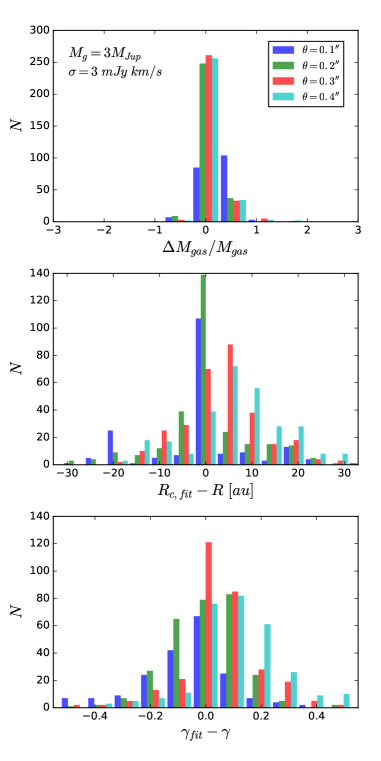
Figure 9: As Figure 8 but for disks with a gas mass $M_{\rm gas}=3\times 10^{-3}\,M_{\odot}$ and noise 3 mJy ${\rm km~{}s^{-1}}$ beam^-1.

Figure 9 plots histograms of the fits for all the disks with a lower mass, $M_{\rm gas}=3\,M_{\rm Jup}=3\times 10^{-2}\,M_{\odot}$, observed at a lower noise level, 3 mJy ${\rm km~{}s^{-1}}$ beam^-1. The results are similar to Figure 8 as might be expected given that the mass and noise level decreased by the same factor of $\sim 3$.

In summary and as a general guideline, the best results are obtained for an intermediate resolution, $0\farcs 2-0\farcs 3$, and once a disk is observed with sufficient signal-to-noise to distinguish it from a gaussian, we find that we can measure the disk size and gradient parameters to within about $\Delta R_{c}=10$ au, $\Delta\gamma=0.2$.

4 Discussion

Unlike the turbulent interstellar medium, the gas structure and kinematics in protoplanetary disks is relatively simple and prescriptive. The complexity in measuring gas masses and surface density profiles resides in the chemistry and radiative transfer required to interpret the observations. CO is an abundant, stable, and readily observable species. Its formation uses almost all available gas-phase C and O and its destruction follows two main pathways, photo-dissociation and freeze-out, that are amenable to semi-analytical models. The intricacies of isotopologue selective dissociation for ¹³CO is largely compensated by the ion-molecule exchange reaction, ¹²CO + ${}^{13}{\rm C}^{+}\longrightarrow\ ^{12}{\rm C}^{+}$ + ¹³CO, deep in the warm molecular layer (Visser et al., 2009). With a good balance between low optical depth and detectability, ¹³CO is the molecule of choice for measuring the gas mass distribution. Finally, because the ordered Keplerian rotation largely separates the emission from different parts of a disk into different spectral channels, we can compare model images to integrated intensity line maps without great loss of information, simplifying and speeding up the fitting process considerably.

Any mass or column density measurement that is derived from observations of a trace molecule fundamentally relies on knowledge of that molecule’s abundance relative to H₂. We assume that the [¹²CO]/[H₂] abundance is the same ($10^{-4}$) in disks as in molecular clouds and cores. There are, unfortunately, few tests of this and they disagree. France et al. (2014) directly measure the abundance from absorption lines through a flared, inclined disk and show agreement with the ISM value. On the other hand, comparison of HD and CO isotopologue lines in the TW Hya disk led Favre et al. (2013) to a much lower abundance. They attributed this to an active carbon chemistry that removes CO from the warm molecular layer and locks up volatiles on large dust grains in the cold midplane (see also Kama et al., 2016). This is a fascinating suggestion that should be testable with more complete inventories of disk gas and statistical studies of gas evolution. Of course, any uncertainty in the global CO abundance translates into the normalization, but not the shape, of the surface density profile.

Our ability to fit the integrated intensity map of ¹³CO 2–1 in the large, bright HD 163296 disk demonstrates the feasibility of our modeling procedure. Although our formal errors were small, our derived surface density profile differs from fits to the ¹²CO 3–2 map by Rosenfeld et al. (2013) and de Gregorio-Monsalvo et al. (2013). The ¹²CO line has a much higher optical depth, however, and and the primary focus of these two studies was on the temperature rather than density structure. A more holistic approach would be to analyze both lines to simultaneously determine the temperature and density structure. By allowing for variation in the the temperature, we would also expect larger errors in the surface density parameters than we report in this proof-of-concept study.

Most stars are lower mass than HD 163926 and most disks are corresponding less massive and also smaller. The first large study designed to measure disk gas masses in a representative sample is the ALMA Lupus survey by Ansdell et al. (2016). They found a very low median gas mass, $M_{\rm gas}\sim 1\,M_{\rm Jup}=10^{-3}\,M_{\odot}$, and the ¹³CO maps have much lower image fidelity than that of HD 163296. The T Tauri grid described in §3 shows that we can extend the same modeling technique, at least for the upper end of that sample, $M_{\rm gas}\gtrsim 3\,M_{\rm Jup}$, through higher resolution, higher sensitivity observations. For the ¹³CO 2–1 line, the requirement is a resolution of $0\farcs 2-0\farcs 3$ and a (mass dependent) noise level of 3–10 mJy ${\rm km~{}s^{-1}}$ beam^-1. The lower rms is achieved with ALMA in 20 minutes so line imaging surveys to determine disk gas surface density profiles are quite feasible in moderate amounts of time. Furthermore the 2–1 lines of both ¹²CO and C¹⁸O can be simultaneously observed with the Band 6 receivers. This is potentially a very powerful combination that permits the co-modeling of temperature and density and the study of selective photo-dissociation. The determination of the gas properties in this way would also provide an essential reference for measuring the abundance and distribution of other molecules.

There have been numerous surveys of the continuum emission from disks and analyses of their solid content. Studies of the disk gas content and distribution provides an additional observational dimension for following their diverse evolutionary pathways. As we gain a more complete picture of both components, gas and dust, we can hope to better understand planet formation and the tremendous range of exoplanet types.

Figure 1: The distribution of posterior probabilities in the MCMC fitting of the ¹³CO integrated intensity map of HD 163296. The three free parameters, gas mass, characteristic radius and surface density gradient are all well constrained.

References

- Aikawa et al. (2002) Aikawa, Y., van Zadelhoff, G. J., van Dishoeck, E. F., & Herbst, E. 2002, A&A, 386, 622
- Andrae et al. (2010) Andrae, R., Schulze-Hartung, T., & Melchior, P. 2010, ArXiv e-prints, arXiv:1012.3754
- Andrews & Williams (2007) Andrews, S. M., & Williams, J. P. 2007, ApJ, 659, 705
- Andrews et al. (2010) Andrews, S. M., Wilner, D. J., Hughes, A. M., Qi, C., & Dullemond, C. P. 2010, ApJ, 723, 1241
- Ansdell et al. (2016) Ansdell, M., Williams, J. P., van der Marel, N., et al. 2016, ArXiv e-prints, arXiv:1604.05719
- Armitage (2013) Armitage, P. J. 2013, Astrophysics of Planet Formation
- Astropy Collaboration et al. (2013) Astropy Collaboration, Robitaille, T. P., Tollerud, E. J., et al. 2013, A&A, 558, A33
- Beckwith & Sargent (1993) Beckwith, S. V. W., & Sargent, A. I. 1993, ApJ, 402, 280
- de Gregorio-Monsalvo et al. (2013) de Gregorio-Monsalvo, I., Ménard, F., Dent, W., et al. 2013, A&A, 557, A133
- Favre et al. (2013) Favre, C., Cleeves, L. I., Bergin, E. A., Qi, C., & Blake, G. A. 2013, ApJ, 776, L38
- Foreman-Mackey et al. (2013) Foreman-Mackey, D., Hogg, D. W., Lang, D., & Goodman, J. 2013, PASP, 125, 306
- France et al. (2014) France, K., Herczeg, G. J., McJunkin, M., & Penton, S. V. 2014, ApJ, 794, 160
- Helled & Bodenheimer (2014) Helled, R., & Bodenheimer, P. 2014, ApJ, 789, 69
- Kama et al. (2016) Kama, M., Bruderer, S., Carney, M., et al. 2016, A&A, 588, A108
- Lay et al. (1997) Lay, O. P., Carlstrom, J. E., & Hills, R. E. 1997, ApJ, 489, 917
- Lynden-Bell & Pringle (1974) Lynden-Bell, D., & Pringle, J. E. 1974, MNRAS, 168, 603
- McKeegan et al. (2011) McKeegan, K. D., Kallio, A. P. A., Heber, V. S., et al. 2011, Science, 332, 1528
- Miotello et al. (2014) Miotello, A., Bruderer, S., & van Dishoeck, E. F. 2014, A&A, 572, A96
- Panić et al. (2009) Panić, O., Hogerheijde, M. R., Wilner, D., & Qi, C. 2009, A&A, 501, 269
- Piétu et al. (2014) Piétu, V., Guilloteau, S., Di Folco, E., Dutrey, A., & Boehler, Y. 2014, A&A, 564, A95
- Pontoppidan et al. (2008) Pontoppidan, K. M., Blake, G. A., van Dishoeck, E. F., et al. 2008, ApJ, 684, 1323
- Qi et al. (2011) Qi, C., D’Alessio, P., Öberg, K. I., et al. 2011, ApJ, 740, 84
- Rosenfeld et al. (2013) Rosenfeld, K. A., Andrews, S. M., Hughes, A. M., Wilner, D. J., & Qi, C. 2013, ApJ, 774, 16
- van Dishoeck & Black (1988) van Dishoeck, E. F., & Black, J. H. 1988, ApJ, 334, 771
- Visser et al. (2009) Visser, R., van Dishoeck, E. F., & Black, J. H. 2009, A&A, 503, 323
- Williams & Best (2014) Williams, J. P., & Best, W. M. J. 2014, ApJ, 788, 59
- Williams & Cieza (2011) Williams, J. P., & Cieza, L. A. 2011, ARA&A, 49, 67