Entanglement of four-qubit systems: a geometric atlas with polynomial compass II (the tame world)

Abstract

We propose a new approach to the geometry of the four-qubit entanglement classes depending on parameters. More precisely, we use invariant theory and algebraic geometry to describe various stratifications of the Hilbert space by SLOCC invariant algebraic varieties. The normal forms of the four-qubit classification of Verstraete et al. are interpreted as dense subsets of components of the dual variety of the set of separable states and an algorithm based on the invariants/covariants of the four-qubit quantum states is proposed to identify a state with a SLOCC equivalent normal form (up to qubits permutation).

I Introduction

Entanglement is nowdays considered as a central ressource in quantum information processing. The large amount of work produced since the beginning of the $\text{XXI}^{\text{st}}$ century to understand the nature of entanglement demonstrates the interest of the community in this subject (see the review papersHHHH ; ES and the references therein). The question of the classification of entanglement of pure multipartite quantum states under the group SLOCC (Stochastic Local Operations with Classical Communication) is one of the most prominent challenging problems on the road to the understanding of entanglement. The complexity of this question grows up exponentially with the number of parts composing the quantum system. If the classification problem is completely solved for a few cases, it is known to be out of reach for most general situation (see RefLT5 for a discussion on the computational complexity of the algebraic invariants of five-qubit systems).

The case of the four-qubit Hilbert space is of special importance. First it has generated a large number of papers by itselfVDMV ; CD ; CDGZ ; BDD ; Levay1 ; Levay3 ; LT ; My ; GW . Then, as long as qubits are concerned, it is the only case where the number of SLOCC orbits is infinite but for which there still exists a list of 9 normal forms found by Verstraete et al.VDMV ; CD (6 of them depend on parameters) which, up to permutation of the qubits, parametrize all SLOCC orbits (i.e. up to permutation of the qubits, a given state is in one of the orbit of the 9 families). The four-qubit case also showed up in different contexts like in the study of the black-holes-qubits correspondenceBDL , in the study of graph-statesGJMW and in many quantum communication protocols like error correcting codesGBP . Thus we consider the four-qubit case as rich enough to motivate more investigation and develop new tools which we hope to be useful to study more difficult cases.

This paper is part of a sequence of articlesHLT ; HLT2 where we have investigated the structure of entanglement for small multipartite systems by combining two different approches: on one side we consider classical invariant theory and we try to understand what the invariants, covariants of the multipartite systems tell us about the SLOCC-orbits and, on the other side, we look at the geometrical structure of the space by building SLOCC algebraic varieties. Combining the two approaches, we obtain a stratification of the Hilbert space by SLOCC algebraic varieties (closure of classes or of union of classes) and criteria based on invariants/covariants, to distinguish them. In our first paperHLT we provided a geometric description of all entanglement classes with invariants/covariants criteria for Hilbert spaces with a finite number of orbits. In RefHLT2 we started to consider the four-qubit case by first looking at specific subvarieties of this Hilbert space. The first subvariety we considered was the nullcone, i.e. the variety of states which annihilate all SLOCC invariant polynomials. It turns out that the number of orbits contained in this variety is finite and thus the techniques developped in RefHLT could apply, leading to a classification, of the nilpotent four-qubit states, using covariants. In the same paper we also considered the case of the algebraic variety $\sigma_{3}(X)$, the third secant variety (see below for the definitions), defined by the simultaneous vanishing of $L$ and $M$, the two degree four generators of the ring of SLOCC invariant polynomials (see below for the definition). This latter case already contains an infinite number of orbits.

In this paper we investigate the geometry of the four-qubit Hilbert space by considering specific SLOCC invariant hypersurfaces: the hypersurfaces defined by the vanishing of the invariants of degree four $L,M$ and $N$ and the so-called hyperdeterminantGKZ $\Delta$ of format $2\times 2\times 2\times 2$. The idea of studing the geometry of the hypersurface defined by $\Delta$ to classify entanglement classes appeared ten years ago in the work of MiyakeMy . The paper of Miyake is based on the study of the singular locus of the hypersurface described ten years earlier by Weymann and ZelevinskyWZ . In this article we go further in the description of the stratification of the ambient space by singular locus of the hyperdeterminant. We consider singularities leading to deeper stratas and we are able to establish a connection between the statas of the ambient space defined by the singularities of $\Delta$ and the $9$ families given by Verstraete et al.’s classification. Like in our previous papersHLT ; HLT2 the geometric approach is combined with a classical invariant theory point of view allowing us to identify the strata to which a given state belongs. It leads to an algorithm based on invariants and covariants which provides, up to a qubit permutation, the family and parameters of a representative SLOCC equivalent to a given state.

The paper is organized as follow. In Section II we illustrate how the adjoint representation of $SO(8)$ on its Lie algebra $\mathfrak{so}(8)$ is connected to the SLOCC ($=SL_{2}(\mathbb{C})^{\times 4}$) orbits of $\mathcal{H}=\mathbb{C}^{2}\times\mathbb{C}^{2}\times\mathbb{C}^{2}\times\mathbb{C}^{2}$ by showing that the generators of the ring of invariants of four-qubit can be obtained by restriction of the generators of the $SO(8)$ polynomial invariants on $\mathfrak{so}(8)$. Similarly we show that the discriminant of the adjoint representation of $SO(8)$, also known as the defining equation of the dual of the adjoint variety, leads to the $2\times 2\times 2\times 2$-hyperdeterminant. In the proof, the hyperdeterminant is obtained as the discriminant of a quartic. This quartic depends on the embedding of $\mathcal{H}$ in $\mathfrak{so}(8)$. In Section III we investigate the three quartics corresponding to the three natural embeddings of $\mathcal{H}$ in $\mathfrak{so}(8)$. It leads to a first stratification of the ambient space based on the roots of the quartics. In particular, we show that this stratification provides a diagram of normal forms which is connected to the geometry of a special semiregular polytope: the demitesseract. In Section IV the geometry of SLOCC hypersurfaces corresponding to specific dual varieties is investigated. This section ends with a geometric stratification of the ambient space where the families of the four-qubit classification are in correspondence with geometric stratas. Moreover some of those stratas are given by a simple geometric interpretation in terms of duals of orbits of well known quantum states. Finally, combining Section III and IV we give an algorithm based on invariants and covariants of four-qubit to determine the Verstraete type of a given state. Section VI is dedicated to concluding remarks.

Notations
All along the paper a four-qubit state $\ket{\varphi}$ will be denoted by $\ket{\varphi}=\sum_{i_{1},\dots,i_{4}\in\{0,1\}^{4}}a_{i_{1}\dots i_{4}}\ket{i_{1}\dotsi_{4}}$ where $\ket{i_{1}\dotsi_{4}}$ stand for the vectors of the computational basis. When not specified the Hilbert space $\mathcal{H}$ will be the space of pure four-qubit quantum states, i.e. $\mathcal{H}=\mathbb{C}^{2}\otimes\mathbb{C}^{2}\otimes\mathbb{C}^{2}\otimes\mathbb{C}^{2}$ and the corresponding SLOCC group will be SLOCC=$SL_{2}(\mathbb{C})^{\times 4}$. When we work over the projective space $\mathbb{P}(\mathcal{H})$, an algebraic variety $Z\subset\mathbb{P}(\mathcal{H})$ is defined as the zero locus of a collection of homogeneous polynomials. For any subset $Y\subset\mathbb{P}(V)$, the notation $\overline{Y}$ will refer to the Zariski closureHa .

II Adjoint variety of $SO(8)$

The classification of four-qubit pure states under SLOCC is strongly connected to the Lie algebra $\mathfrak{so}_{8}$. In the original paper of Verstraete et al.VDMV , the action of the $SO(4)\times SO(4)$ subgroup of $SO(8)$, on the space of $8\times 8$ matrices is used to provide a first classification of SLOCC orbits of $\mathcal{H}=\mathbb{C}^{2}\otimes\mathbb{C}^{2}\otimes\mathbb{C}^{2}\otimes\mathbb{C}^{2}$. This idea is made more precise, and the classification corrected, in the work of Chterental and Djoković CD where the Lie algebra $\mathfrak{so}_{8}$ is decomposed under the involution defined by the diagonal matrix $g=\begin{pmatrix}I_{4}&0\\ 0&-I_{4}\end{pmatrix}$:

$$\mathfrak{so}_{8}=\mathfrak{k}\oplus\mathfrak{p}.$$ (1)

The $SO(4)\times SO(4)$ invariant subspace $\mathfrak{p}$ is

$$\mathfrak{p}=\{\begin{pmatrix}0&R\\ -R^{T}&0\end{pmatrix},R\in\mathcal{M}_{4}(\mathbb{C})\}$$ (2)

The action of $SO(4)\times SO(4)$ on $\mathfrak{p}$ corresponds to the action of SLOCC on $\mathcal{H}=\mathbb{C}^{2}\otimes\mathbb{C}^{2}\otimes\mathbb{C}^{2}\otimes\mathbb{C}^{2}$. The correspondence is given as follows. Let $\ket{\varphi}=\sum_{i,j,k,l\in\{0,1\}}a_{ijkl}\ket{ijkl}$ be a four-qubit state. One associates with $\ket{\varphi}$ the $4\times 4$ matrix

$$M_{\varphi}=\begin{pmatrix}a_{0000}&a_{0010}&a_{0001}&a_{0011}\\ a_{1000}&a_{1010}&a_{1001}&a_{1011}\\ a_{0100}&a_{0110}&a_{0101}&a_{0111}\\ a_{1100}&a_{1110}&a_{1101}&a_{1111}\end{pmatrix}.$$ (3)

Let $(A_{1},A_{2},A_{3},A_{4})$ be an element of the group SLOCC$=SL_{2}(\mathbb{C})^{\times 4}$. The action on $M_{\varphi}$ is given by $(A_{1}\otimes A_{2})M_{\varphi}(A_{3}\otimes A_{4})^{t}$. This action on the space of $4\times 4$ matrices becomes an action of $SO(4)\times SO(4)$ on $\mathfrak{p}$. This is described in RefCD via the following unitary matrix (see also Ref VDMV ):

$$T=\dfrac{1}{\sqrt{2}}\begin{pmatrix}1&0&0&1\\ 0&i&i&0\\ 0&-1&1&0\\ i&0&0&-i\end{pmatrix}.$$ (4)

One gets the correspondence: $(A_{1},A_{2},A_{3},A_{4})\in\text{SLOCC}\text{ acts on }\mathcal{H}$ and $\begin{pmatrix}P_{1}&0\\ 0&P_{2}\end{pmatrix}\in SO(4)\times SO(4)$ acts on $\mathfrak{p}$ with $P_{1}=T(A_{1}\otimes A_{2})T^{\dagger}$ and $P_{2}=T(A_{3}\otimes A_{4})T^{\dagger}$ such that

$$A_{1}\otimes A_{2}\otimes A_{3}\otimes A_{4}\ket{\varphi}=\begin{pmatrix}P_{1}&0\\ 0&P_{2}\end{pmatrix}\begin{pmatrix}0&TM_{\varphi}T^{\dagger}\\ -(TM_{\varphi}T^{\dagger})^{t}&0\end{pmatrix}\begin{pmatrix}P_{1}&0\\ 0&P_{2}\end{pmatrix}^{-1}.$$ (5)

The action of $SO(4)\times SO(4)$ on $\mathfrak{p}$ is nothing but the trace of the adjoint action of $SO(8)$ on $\mathfrak{p}$. This embedding of the vector space $\mathcal{H}$ into $\mathfrak{so}_{8}$ leads to the following observation.

Proposition II.1.

Let $\mathbb{C}[\mathfrak{so}_{8}]^{SO(8)}$ be the ring of invariant polynomials on $\mathfrak{so}_{8}$ for the adjoint action of $SO(8)$ and $\mathbb{C}[\mathcal{H}]^{\text{SLOCC}}$ the ring of invariant polynomials for the SLOCC action on the four-qubit Hilbert space. The restriction map

$$\mathbb{C}[\mathfrak{so}_{8}]^{SO(8)}\longrightarrow\mathbb{C}[\mathfrak{p}]^{SO(4)\times SO(4)}=\mathbb{C}[\mathcal{H}]^{\text{SLOCC}}$$ (6)

is an isomorphism. Moreover the restriction of the equation defining the dual variety of the adjoint orbit $X_{SO(8)}\subset\mathbb{P}(\mathfrak{so}_{8})$ to $\mathfrak{p}$ is the $2\times 2\times 2\times 2$ hyperdeterminant.

Proof.

It is well knownPV that the ring of invariant polynomials $\mathbb{C}[\mathfrak{so}_{2n}]^{SO(2n)}$ is a free algebra generated by homogeneous algebraically independent polynomials of degree $2,4,\dots,2(n-1),n$. Let us denote by $\mathcal{M}^{0}_{2n}(\mathbb{C})$ the space of traceless matrices of size $2n\times 2n$, and let us recall that $\mathfrak{so}_{2n}=\{A\in\mathcal{M}^{0}_{2n}(\mathbb{C}),A=-A^{t}\}$. The generators of $\mathbb{C}[\mathfrak{so}_{2n}]^{SO(2n)}$ can be obtained as the restriction to $\mathfrak{so}_{2n}$ of the sum of the $i\times i$ principal minors. For skew symmetric matrices only the even dimensionnal principal minors do not vanish. Moreover the determinant of a skew symmetric matrix factorizes as the square of the Pfaffian, $Pf$. In other words the generators of $\mathbb{C}[\mathfrak{so}_{2n}]^{SO(2n)}$ can be chosen to be $h_{2},\dots,h_{2n-2},Pf$ where $h_{2i}$ is the sum of the $2i\times 2i$ principal minors. In particular if we consider $\mathfrak{so}_{8}$, the generators are four polynomials of degree $2,4,6,4$. The ring of invariant polynomials for four-qubit states under SLOCCLT is also a free algebra generated by homogeneous algebraically independent polynomials of degree $2,4,4,6$. Let us denote them respectively $B,L,M$ and $D$, their descriptions will be given in the next section. The restriction of the sum of principal minors $h_{2},h_{4},h_{6}$ and the Pfaffian $Pf$ to $\mathfrak{p}$, i.e. to the vector space

$$\begin{pmatrix}0&TM_{\varphi}T^{\dagger}\\ -(TM_{\varphi}T^{\dagger})^{t}&0\end{pmatrix}$$ (7)

leads to the following equalities: ${h_{2}}_{|_{\mathfrak{p}}}=2B$, ${h_{4}}_{|_{\mathfrak{p}}}=B^{2}+2L+4M$, ${h_{6}}_{|_{\mathfrak{p}}}=2BL+4BM-4D$ and $Pf_{|_{\mathfrak{p}}}=L$. It immediately proves that ${\mathbb{C}[\mathfrak{so}_{8}]^{SO(8)}}_{|\mathfrak{p}}=\mathbb{C}[\mathcal{H}]^{\text{SLOCC}}$.

Regarding the dual variety of $X_{SO(8)}\subset\mathbb{P}(\mathfrak{so}_{8})$, we recall that an equation of $X_{SO(2n)}^{*}$ is known in terms for the simple roots of the Lie algebras $\mathfrak{so}_{2n}$. In fact for all simple Lie algebras the equation defining the dual of the projectivization of the adjoint orbit is given by the vanishing of the discriminant $D_{\mathfrak{g}}$, i.e. the product of the (long) roots of $\mathfrak{g}$ (see RefTev p29).

$$D_{\mathfrak{g}}=\prod_{\alpha\in R_{l}}\alpha=0$$ (8)

Let $M\in\mathfrak{so}_{8}$ and $M_{s}$ its semi-simple part with eigenvalues $\lambda_{1},\dots,\lambda_{n}$. The rootsF-H of $\mathfrak{so}_{2n}$ are linear forms on $\mathfrak{h}$, the Cartan subalgebra of $\mathfrak{so}_{2n}$, of the form $\pm L_{i}\pm L_{j}$ with $i\neq j$ and such that $L_{i}(M_{s})=\lambda_{i}$. Thus if $\alpha$ is a root we have $\alpha(M_{s})=\pm\lambda_{i}\pm\lambda_{j}$ and the matrix $M\in\mathfrak{so}_{2n}$ belongs to $X_{SO_{2n}}^{*}$ if and only if

$$D_{l}(M)=\prod_{1\leq i<j\leq n,i\neq j}(\lambda_{i}\pm\lambda_{j})^{2}=0.$$ (9)

The roots of the characteristic polynomial of $M$, $t^{2n}+h_{2}(M)t^{2n-2}+\dots+h_{2n-2}(M)t^{2}+Pf^{2}(M)$ are $\pm\lambda_{i}$. Using the change of variable $x=t^{2}$, one gets the polynomial

$$x^{n}+h_{2}(M)x^{n-1}+\dots+h_{2n-2}(M)x+Pf^{2}(M)$$ (10)

whose roots are $\lambda_{i}^{2}$. Taking the discriminant one obtains:

$$\Delta(x^{n}+h_{2}(M)x^{n-1}+\dots+h_{2n-2}(M)x+Pf^{2}(M))=\prod_{1\leq i<j\leq n}(\lambda_{i}^{2}-\lambda_{j}^{2})^{2}=\prod_{1\leq i<j\leq n,i\neq j}(\lambda_{i}\pm\lambda_{j})^{2}$$ (11)

One concludes that $\Delta(x^{n}+h_{2}(M)x^{n-1}+\dots+h_{2n-2}(M)x+Pf^{2}(M))=D_{\mathfrak{so}_{2n}}(M)$.

In particular $\Delta(x^{4}+h_{2}(M)x^{3}+h_{4}(M)x^{2}+h_{6}(M)x+Pf^{2}(M))=0$ is the defining equation of $X_{SO(8)}^{*}$. But it can also be checked that $\Delta(x^{4}+2Bx^{3}+(B^{2}+2L+4M)x^{2}+(2BL+4BM-4D)x+L^{2})=0$ is an equation for the dual variety of $\mathbb{P}^{1}\times\mathbb{P}^{1}\times\mathbb{P}^{1}\times\mathbb{P}^{1}$, i.e. $\Delta(x^{4}+2Bx^{3}+(B^{2}+2L+4M)x^{2}+(2BL+4BM-4D)x+L^{2})$ is the hyperdeterminant of format $2\times 2\times 2\times 2$. $\Box$

Remark II.1.

The connection between the SLOCC orbit structure of four-qubits and the Lie algebra $\mathfrak{so}_{8}$ is also investigated in a different manner in the work of Péter LévayLevay1 ; Levay2 and more recently in RefLevay3 with a construction of the four-qubit invariants from the spin representation of $SO(16)$. From a different perspective a connection between four-qubit states and the Dynkin diagram $D_{4}$ (the Dynkin diagram of $\mathfrak{so}_{8}$) was also pointed out in RefHLP by constructing simple hypersurface singularities of type $D_{4}$ and their deformations from four-qubit states.

Remark II.2.

The embedding of $\mathcal{H}$ as a subspace of $\mathfrak{so}_{8}$ depends on the embedding of the four-qubit state $\ket{\varphi}$ in $\mathcal{M}_{4}(\mathbb{C})$ given by Eq (3). There are two more ways of looking at a four-qubit state as a linear map from $\mathbb{C}^{4}$ to $\mathbb{C}^{4}$. Those other two representations will give different ways of writing the generators of $\mathbb{C}[\mathcal{H}]^{\text{SLOCC}}$, but also two different types of quartics like the one given by Eq (10) for $n=4$. In the next section their role in the classification of the SLOCC orbits is investigated.

III A first classification based on invariants

III.1 SLOCC-invariant polynomials

In a general setting, a pure $k$-qudit state is an element of the Hilbert space $\mathcal{H}=V_{1}\otimes\cdots\otimes V_{k}$ with $V_{i}=\mathbb{C}^{n_{i}}$ regarded as a multilinear form. Two qudit states are equivalent if they belong to the same orbit for the group $\mathrm{SLOCC}=GL_{n_{1}}\times\cdots\times GL_{n_{k}}$. In principle, one can determine if two states are equivalent by comparing their evaluations on a sufficiently large system of special polynomials (in the coefficients of the forms and auxiliary variables), called concomitants, which are invariant under the action of $\mathrm{SLOCC}$. In practice, this algorithm can be used only in very few cases, because the number and the size of the polynomials increase exponentially with the number of particles and the dimension of the Hilbert space. Nevertheless, even the knowledge of a little part of the polynomials gives rise to interesting information about the classification.

In the case of a four-qubit system, we deal with the quadrilinear form:

$$f:=\sum_{0\leq i,j,k,\ell\leq 1}a_{ijk\ell}x_{i}y_{j}z_{k}t_{\ell}$$ (12)

and the algebra of the polynomial invariants (polynomials in the coefficients of the forms with no auxiliary variables) is a free algebra on four generators:

1. One of degree 2:

   $$\begin{array}[]{rcl}B&:=&a_{0000}a_{1111}-a_{1000}a_{0111}+a_{0100}a_{1011}+a_{1100}a_{0011}-a_{0010}a_{1101}\\ &&+a_{1010}a_{0101}-a_{0110}a_{1001}+a_{1110}a_{0001},\end{array}$$ (13)

2. two of degree 4:

   $$L:=\left|\begin{array}[]{cccc}a_{0000}&a_{0010}&a_{0001}&a_{0011}\\ a_{1000}&a_{1010}&a_{1001}&a_{1011}\\ a_{0100}&a_{0110}&a_{0101}&a_{0111}\\ a_{1100}&a_{1110}&a_{1101}&a_{1111}\end{array}\right|\mbox{ and }M:=\left|\begin{array}[]{cccc}a_{0000}&a_{0001}&a_{0100}&a_{0101}\\ a_{1000}&a_{1001}&a_{1100}&a_{1101}\\ a_{0010}&a_{0011}&a_{0110}&a_{0111}\\ a_{1010}&a_{1011}&a_{1110}&a_{1111}\end{array}\right|$$ (14)

3. and one of degree 6: Set $b_{xy}:=\det\left(\dfrac{\partial^{2}f}{\partial z_{i}\partial t_{j}}\right)$. By interpreting this quadratic form as a bilinear form on the three dimensional space, one finds a $3\times 3$ matrix $B_{xy}$ satisfying $b_{xy}=[x_{0}^{2},x_{0}x_{1},x_{1}^{2}]B_{xy}\left[\begin{array}[]{c}y_{0}^{2}\\ y_{0}y_{1}\\ y_{1}^{2}\end{array}\right].$ The generator of degree $6$ is

   $$D_{xy}:=-\det(B_{xy}).$$ (15)

Remark that this set is not unique, for instance one can replace $L$ or $M$ by

$$N:=-L-M=\left|\begin{array}[]{cccc}a_{0000}&a_{1000}&a_{0001}&a_{1001}\\ a_{0100}&a_{1100}&a_{0101}&a_{1101}\\ a_{0010}&a_{1010}&a_{0011}&a_{1011}\\ a_{0110}&a_{1110}&a_{0111}&a_{1111}\end{array}\right|.$$ (16)

We remark that, when evaluated on the Verstraete normal form VDMV

$$\begin{array}[]{rcl}G_{abcd}&:=&\frac{1}{2}(a+d)(|0000\rangle+|1111\rangle)+\frac{1}{2}(a-d)(|1100\rangle+|0011\rangle)+\\ &&\frac{1}{2}(b+c)(|0101\rangle+|1010\rangle)+\frac{1}{2}(b-c)(|0110\rangle+|0011\rangle,\end{array}$$ (17)

these invariants have nice closed expressions:

$$B(|G_{abcd}\rangle)=\frac{1}{2}\left(a^{2}+b^{2}+c^{2}+d^{2}\right),$$ (18)

$$L(|G_{abcd}\rangle)=abcd,$$ (19)

$$M(|G_{abcd}\rangle)=\frac{1}{16}(a+b+c+d)(c+d-a-b)(a-b+c-d)(a-b+d-c),$$ (20)

$$N(|G_{abcd}\rangle)=\frac{1}{16}(a+b+c-d)(a-b-c-d)(a-b+c+d)(a+b-c+d),$$ (21)

$$D_{xy}(|G_{abcd}\rangle)=\frac{1}{32}\,\left({b}^{2}-{a}^{2}+{c}^{2}-{d}^{2}\right)\left(-{b}^{2}+{a}^{2}+{c}^{2}-{d}^{2}\right)\left({b}^{2}+{a}^{2}-{c}^{2}-{d}^{2}\right).$$ (22)

We consider the space $\mathcal{S}:=\left\{\left|G_{abcd}\right\rangle:(a,b,c,d)\in\mathbb{C}^{4}\right\}$ of the Verstraete normal forms. It is the Chevalley section for the $\mathrm{SLOCC}$ action on the Hilbert space with Weyl group $D_{4}$: the closure of each generic orbit intersects $\mathcal{S}$ along a $D_{4}$ orbit. Indeed, since the polynomials $B(|G_{abcd}\rangle)$, $L(|G_{abcd}\rangle)$, $M(|G_{abcd}\rangle)$, and $D_{xy}(|G_{abcd}\rangle)$ are algebraically independent, the system

$$\left\{\begin{array}[]{l}B(|G_{abcd}\rangle)=\alpha\\ L(|G_{abcd}\rangle)=\beta\\ M(|G_{abcd}\rangle)=\gamma\\ D_{xy}(|G_{abcd}\rangle)=\delta\end{array}\right.$$ (23)

admits at most $192$ solutions (this is the order of $D_{4}$). Furthermore, the system is clearly invariant under the permutations of the variables $(a,b,c,d)$ and the transformation $(a,b)\longrightarrow(-a,-b)$. For generic values of $(a,b,c,d)$, these transformations generate a group isomorphic to $D_{4}$. Hence, knowing one solution, the other ones are deduced from the action of $D_{4}$. Geometrically, the solutions are symmetric with respect to the reflection group of the demitesseract. See Appendix A.

III.2 Three quadrics

We consider the three quartics

$$Q_{1}(|\varphi\rangle):=x^{4}-2Bx^{3}y+(B^{2}+2L+4M)x^{2}y^{2}+(4D_{xy}-4B(M+\frac{1}{2}L))xy^{3}+L^{2}y^{4},$$ (24)

$$Q_{2}(|\varphi\rangle):=x^{4}-2Bx^{3}y+(B^{2}-4L-2M)x^{2}y^{2}+(-2MB+4D_{xy})xy^{3}+M^{2}y^{4},$$ (25)

$$Q_{3}(|\varphi\rangle):=x^{4}-2Bx^{3}y+(B^{2}+2L-2M)x^{2}y^{2}-(2LB+2MB-4D_{xy})xy^{3}+N^{2}y^{4}.$$ (26)

Evaluated on $|G_{abcd}\rangle$, the roots of $Q_{1}$ are $a^{2}$, $b^{2}$, $c^{2}$ and $d^{2}$ and the roots of $Q_{2}$ (resp. $Q_{3}$) are the squares of the four polynomial factors of $M(|G_{abcd}\rangle)$ (resp. $N(|G_{abcd}\rangle)$ which are obtained by applying an invertible linear transformation to $(a,b,c,d)$. Hence, the three quartics have the same invariants.
The invariant polynomials of a quartic $f:=\alpha x^{4}-4\beta x^{3}y+6\gamma x^{2}y^{2}-4\delta xy^{3}+\omega y^{4}$ are algebraic combinations of $I_{2}=\alpha\omega-4\beta\delta+3\gamma^{2}$, an invariant of degree $2$, which is the apolar of the form with itself, and $I_{3}=\alpha\gamma\omega-\alpha\delta^{2}-\beta^{2}\omega-\gamma^{3}+2\beta\gamma\omega$, an invariant of degree $3$ called the catalecticantOlver . In particular, the discriminant of the quadric is $\Delta=I_{2}^{3}-27I_{3}^{2}$.
From these definitions, one has

$$I_{2}(Q_{1})=I_{2}(Q_{2})=I_{2}(Q_{3})=\frac{4}{3}\,{{L}}^{2}+2\,{B}\,{D_{xy}}-\frac{4}{3}\,{{B}}^{2}{M}-\frac{2}{3}\,{{B}}^{2}{L}+\frac{1}{12}\,{{B}}^{4}+\frac{4}{3}\,{L}\,{M}+\frac{4}{3}\,{{M}}^{2},$$ (27)

and

$$\begin{array}[]{rcl}I_{3}(Q_{1})=I_{3}(Q_{2})=I_{3}(Q_{3})&=&\frac{4}{2}\,{D_{xy}}\,{B}\,{M}+\frac{2}{3}\,{D_{xy}}\,{B}\,{L}-\frac{5}{9}\,{{B}}^{2}{M}\,{L}+\frac{4}{9}\,{L}^{2}{M}-{{D_{xy}}}^{2}-\frac{5}{9}\,{{B}}^{2}{{M}}^{2}\\ &&+\frac{1}{18}\,{B}^{4}{L}+\frac{1}{9}\,{B}^{4}{M}-\frac{4}{9}\,{L}\,{{M}}^{2}-\frac{1}{6}\,{{B}}^{3}{D_{xy}}-\frac{2}{9}\,{{B}}^{2}{{L}}^{2}+{\frac{8}{27}}\,{{L}}^{3}\\ &&-{\frac{1}{216}}\,{{B}}^{6}-{\frac{8}{27}}\,{{M}}^{3}.\end{array}$$ (28)

Furthermore, we easily check that $\Delta(Q_{i})$ is also the hyperdeterminant of $|\varphi\rangle$ (regarded as a quadrilinar form).
In the aim to describe the roots of the quartics, we will use two other covariant polynomials: the Hessian

$$Hess(f):=\left|\begin{array}[]{cc}{\partial^{2}\over\partial x^{2}}f&{\partial^{2}\over\partial x\partial y}f\\ {\partial^{2}\over\partial y\partial x}f&{\partial^{2}\over\partial y^{2}}f\end{array}\right|$$ (29)

and the Jacobian of the Hessian

$$T(f)=\left|\begin{array}[]{cc}{\partial\over\partial x}f&{\partial\over\partial y}f\\ {\partial\over\partial x}Hess(f)&{\partial\over\partial y}Hess(f)\end{array}\right|.$$ (30)

From the values of the covariants one can compute the multiplicity of the roots of a quartic $f$, according to Table 1.

$$\begin{array}[]{|c|l|}\hline\cr Covariants&Interpretation\\ \hline\cr\Delta\neq 0&\mbox{ Four distinct roots}\\ \Delta=0\mbox{ and }T\neq 0&\mbox{ Exactly one double root}\\ T=0\mbox{ and }I_{2}\neq 0&\mbox{ Two distinct double roots}\\ I_{2}=I_{3}=0\mbox{ and }Hess\neq 0&\mbox{ A triple root}\\ Hess=0&\mbox{ A quadruple root}\\ \hline\cr\end{array}$$

Table 1: Roots of a quartic

Notice that the evaluations of $Hess$ and $T$ on the forms $Q_{1}$, $Q_{2}$ and $Q_{3}$ are not equal in the general case.

III.3 A first classification

In this section, we use Table 1 to obtain a first classification and we refine it by considering the polynomials $L$, $M$ and $N$ which allow to decide if a quartic has a null root. The discussion is relegated to Appendix B.
We define the invariants

$$P:=D_{xy}-BM,S_{1}:=B^{2}+4M,S_{2}=B^{2}-4L,\mbox{ and }S_{3}=B^{2}-4M.$$ (31)

If $S$ is a set of polynomials, we will denote by $\mathcal{V}_{S}$ the variety defined by the system $\{E=0:E\in S\}$. In a previous paperHLT2 , we have investigated the case when $L=M=0$. It remains to consider the other cases and, according to Appendix B, one has to refine the diagram of inclusions of Figure 1 which represents a first tentative of classification (see also Figure 2 for the interpretation of red part in terms of roots of the quartics). The green part corresponds to subvarieties of $\mathcal{V}_{L,M}$ that are already investigated in a previous paperHLT2 . Also, notice that the whole diagram of Figure 1 can be deduced from the red part, replacing $L=0$ by $M=0$ (resp. $N=0$). Note that $\mathcal{V}_{L,P,S_{1},I_{2},I_{3}}=\mathcal{V}_{L,P,S_{1}}$. Indeed, for any form in $\mathcal{V}_{L,P,S_{1},I_{2},I_{3}}$, $Q_{1}$ has a zero triple root and this implies automatically that $Q_{2}$ has a quadruple root which is equal to one of the parameter of the normal form. The case where one of the quartic has two double roots does not appear explicitly in the diagrams. But, a short calculation shows that it is equivalent to the case where one of the quartics has zero as a double root.

Figure 1: Inclusion diagram of the varieties $\mathcal{V}_{S}$.

Figure 2: Interpretation of the red part of Figure 1 in terms of quartics.

III.4 The form problem again

Each of the varieties described in Figure 1 contains orbits whose intersections with the Chevalley section $\mathcal{S}$ are finite sets of points with symmetries related to some four dimensional polytopes.

• A generic orbit in $\mathcal{V}_{\emptyset}$ intersect $\mathcal{S}$ in $192$ points splitting into $8$ subsets of $24$ points belonging to the same hyperplane. Each of these subsets is constituted with the permutations of the same vector $(a,b,c,d)$ and centered on one of the vertices of a demitesseract (see Figure 3).

  

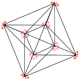
  Figure 3: Intersection of a generic orbit of $\mathcal{V}_{\emptyset}$ with the subspace of normal forms.

• In $\mathcal{V}_{L}$, each generic orbit contains also $192$ normal forms which are the permutations of the same vector $(0,a,b,c)$. The set of the normal forms splits into $32$ subsets which are constituted of $6$ points, belonging to the same space of dimension $2$, centered on one of the points $(\alpha,\alpha,\alpha,0)$, $(\alpha,\alpha,0,\alpha)$, $(\alpha,0,\alpha,\alpha)$ or $(0,\alpha,\alpha,\alpha)$ with $\alpha={\pm a\pm b\pm c\over 3}$, that are middles of the edges of a tesseract (see Figure 4).

  

  

  Figure 4: Intersection of a generic orbit of $\mathcal{V}_{L}$ with the subspace of normal forms and the tesseract.

• A generic orbit in $\mathcal{V}_{\Delta}$ is a special orbit in $\mathcal{V}_{\emptyset}$ with $96$ normal forms splitting into $8$ subsets of $12$ points.
  

• A generic orbit in $\mathcal{V}_{\Delta,L}$ is a special orbit in $\mathcal{V}_{L}$ with $96$ normal forms splitting into $32$ subsets of $3$ points centered on the middle of the edges of a tesseract (see Figure 5).
  

  

  Figure 5: Intersection of a generic orbit of $\mathcal{V}_{\Delta,L}$ with the subspace of normal forms.

• A generic orbit in $\mathcal{V}_{I_{2},I_{3}}$ is a special orbit in $\mathcal{V}_{\Delta}$ with $24$ normal forms splitting into $8$ subsets of $4$ points.

• A generic orbit in $\mathcal{V}_{L,P}$ is a special orbit in $\mathcal{V}_{L,\Delta}$ with $48$ normal forms splitting into $24$ pairs of points whose the middles are the vertices of a $24$-cell polytope (see Figure 6). These vertices are also the centers of the faces of a tesseract. Notice that such an orbit can degenerate and have only $24$ normal forms, which are exactly the vertices of the $24$-cell. In this case, one has $T(Q_{1})=0$ (because $Q_{1}$ has two double roots). From Appendix B, it follows that $L=M=0$ and, since this case has already been investigated in one of our previous papers, we will not examine it here.

  

  

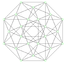
  Figure 6: Intersection of a generic orbit of $\mathcal{V}_{L,P}$ with the subspace of normal forms and a $24$-cell polytope.

• A generic orbit in $\mathcal{V}_{L,P,S_{1}}$ is a special orbit in $\mathcal{V}_{L,P}$ with $16$ normal forms, which are the vertices of a $16$-cell polytope (see Figure 7).

  

  

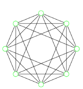
  Figure 7: Intersection of a generic orbit of $\mathcal{V}_{L,P,S_{1}}$ with the subspace of normal forms and a $16$-cell polytope.

Hence, one can interpret the diagram of Figure 1 in terms of normal forms in Figure 8.

Figure 8: Diagram of normal forms.

Let us end the discussion by an illustration of the fact that the quartics $Q_{1}$, $Q_{2}$ and $Q_{3}$ have an interchangeable role: we first remark that one can choose a degenerate orbit in $\mathcal{V}_{\emptyset}$ by setting $a=b=c=d$. In this case, the normal forms are the vertices of the demitesseract and so of a $16$-cell. It is similar (up to a rotation) to a generic orbit in $\mathcal{V}_{L,\Delta,P,Q}$. In terms of quartics, this is interpreted by the fact that $Q_{1}$ has a quadruple root and $Q_{2}$ has a zero triple root (compare to the variety $\mathcal{V}_{L,\Delta,P,Q}$, where $Q_{1}$ has a zero triple root and $Q_{2}$ has a quadruple root).

IV Classification based on geometric stratification

We now investigate the SLOCC structure of the four-qubit Hilbert space from a geometrical point of view. Because a quantum state is well-defined up to a phase factor we will consider the projective Hilbert space $\mathbb{P}(\mathcal{H})=\mathbb{P}(\mathbb{C}^{2}\otimes\mathbb{C}^{2}\otimes\mathbb{C}^{2}\otimes\mathbb{C}^{2})$ and we recall that $X=\mathbb{P}^{1}\times\mathbb{P}^{1}\times\mathbb{P}^{1}\times\mathbb{P}^{1}$, the Segre embedding of four projective lines, is the variety of separable statesHLT . We begin the section by defining the auxiliary varieties already used in our previous workHLT ; HLT2 to describe SLOCC invariant varieties built from the knowledge of $X$. Then we look at various stratifications of the ambient space induced by the singular locus of the four hypersurfaces corresponding to the zero locus of $L,M,N$ and $\Delta$. When combined, we recover the stratification induced by the three quartics $Q_{1},Q_{2}$ and $Q_{3}$.

IV.1 Secant, tangent and dual varieties

The basic geometric tool introduced in our previous papersHLT ; HLT2 was the concept of auxiliary varieties. An auxiliary variety is an algebraic variety built by elementary geometric constructions from a given variety. An example of such is the so called secant varietyZ2 ; Lan3 . If $Y\subset\mathbb{P}(V)$ is a projective variety, the secant variety of $Y$ is the algebraic closure of the union of secant lines:

$$\sigma(Y)=\overline{\bigcup_{x,y\in Y}\mathbb{P}^{1}_{xy}}.$$ (32)

If $Y=X$, the set of separable states, then $\sigma(X)$ is the algebraic closure of quantum states which are sums of two separable states. This algebraic variety is SLOCC invariant because so is $X$ and it can be shown, for any multipartite system, that $\sigma(X)=\overline{\text{SLOCC}\ket{GHZ}}$ where $\ket{GHZ}$ is the usual generalization of the GHZ-state and $X$ still denotes the variety of separable states.

In the same spirit, higher dimensional secant varieties can be defined by

$$\sigma_{k}(Y)=\overline{\bigcup_{x_{1},\dots,x_{k}\in Y}\mathbb{P}^{k-1}_{x_{1},\dots,x_{k}}}.$$ (33)

The secant varieties naturally provides a stratification of the ambient space and states belonging to different secant varieties can not be SLOCC equivalent. The interest of secant varieties in the context of quantum entanglement was first pointed out by Heydarihey .

Another auxiliary variety of importance is the so-called tangential variety which corresponds to the union of tangent lines. If $Y$ is a smooth variety and $\tilde{T}_{y}Y$ denotes the embedded tangent space of $Y$ at $y$ we have.

$$\tau(Y)=\bigcup_{y\in Y}\tilde{T}_{y}Y.$$ (34)

This variety has also a nice quantum information theory interpretation. For any multipartite system we have, if $X$ still denotes the variety of separable states, $\tau(X)=\overline{\text{SLOCC}\ket{W}}$ where $\ket{W}$ is the generalization of the W-states. Those are well-known fact from algebraic geometryZ2 ; Lan3 and have been restated in the language of quantum information theory in RefHL .

In our geometric description of the stratification of the ambient space by algebraic varieties we will also use the concept of dual variety. Let us remind what the dual variety of a projective algebraic variety is, and why this concept has been already introduced in the study of entanglement of multipartite systemsMy ; HLT .

Consider $X\subset\mathbb{P}(V)$ a nondegenerate projective variety (i.e. not contained in a hyperplane). The dual variety of $X$ is the closure of the set of tangent hyperplanes, i.e. is defined by

$$X^{*}=\overline{\{H\in\mathbb{P}(V^{*}),\exists x\in X_{\text{smooth}},\tilde{T}_{x}X\subset H\}}$$ (35)

where $\tilde{T}_{x}X$ denote the embedded tangent space of $X$ at $x$ (see RefLan ).

If $X$ is a $G$-invariant variety for a $G$-action on $V$ and $X^{*}$ is a hypersurface, then the defining equation of $X^{*}$ is a $G$-invariant polynomial. In the case of $X=\mathbb{P}^{k_{1}}\times\dots\times\mathbb{P}^{k_{r}}$ with $k_{1}\leq k_{2}+\dots+k_{r}$ (assuming $k_{1}\geq k_{i}$) the dual variety is always a hypersurface called the hyperdeterminant of format $(k_{1}+1)\times(k_{2}+1)\times\dots\times(k_{r}+1)$ and it is a $G=GL_{k_{1}+1}\times\dots\times GL_{k_{r}+1}$-invariant polynomial. Hyperdeterminants have been deeply studied by Gelfand Kapranov and ZelevinskyGKZ1 ; GKZ .

In the case where $X=\mathbb{P}^{1}\times\mathbb{P}^{1}\times\mathbb{P}^{1}$, the hyperdeterminant of format $2\times 2\times 2$ is the so-called Cayley hyperdeterminant and when $X=\mathbb{P}^{1}\times\mathbb{P}^{1}\times\mathbb{P}^{1}\times\mathbb{P}^{1}$, the hyperdeterminant is the invariant polynomial $\Delta$ introduced in Section III.

Other SLOCC invariant polynomials, or SLOCC invariant algebraic varieties of the Hilbert space of four qubits can be interpreted in terms of dual varieties as we now show.

IV.2 The hypersufaces $\{L=0\}$, $\{M=0\}$ and $\{N=0\}$

The three hypersurfaces defined by the vanishing of one of the quartic invariant polynomials $L$, $M$ or $N$ are isomorphic and correspond to the dual varieties of three different types of embeddings of $\mathbb{P}^{3}\times\mathbb{P}^{3}$ in $\mathbb{P}^{15}=\mathbb{P}(\mathbb{C}^{2}\otimes\mathbb{C}^{2}\otimes\mathbb{C}^{2}\otimes\mathbb{C}^{2})$.

Indeed, let $A,B\in\mathbb{C}^{2}\otimes\mathbb{C}^{2}$ be two $2\times 2$ matrices which are tensors of rank at most two, i.e. $A=t_{1}\otimes u_{1}+t_{2}\otimes u_{2}$ and $B=v_{1}\otimes w_{1}+v_{2}\otimes w_{2}$. Then we have the following three embeddings:

$$\begin{array}[]{cccc}&\mathbb{P}^{3}\times\mathbb{P}^{3}&\hookrightarrow&\mathbb{P}^{15}\\ \phi_{1}:&([A],[B])&\hookrightarrow&[t_{1}\otimes u_{1}\otimes v_{1}\otimes w_{1}+t_{1}\otimes u_{1}\otimes v_{2}\otimes w_{2}\\ &&&+t_{2}\otimes u_{2}\otimes v_{1}\otimes w_{1}+t_{2}\otimes u_{2}\otimes v_{2}\otimes w_{2}]\\ \phi_{2}:&([A],[B])&\hookrightarrow&[w_{1}\otimes u_{1}\otimes v_{1}\otimes t_{1}+w_{1}\otimes u_{1}\otimes v_{2}\otimes t_{2}\\ &&&+w_{2}\otimes u_{2}\otimes v_{1}\otimes t_{1}+w_{2}\otimes u_{2}\otimes v_{2}\otimes t_{2}]\\ \phi_{3}:&([A],[B])&\hookrightarrow&[t_{1}\otimes v_{1}\otimes u_{1}\otimes w_{1}+t_{1}\otimes v_{1}\otimes u_{2}\otimes w_{2}\\ &&&+t_{2}\otimes v_{2}\otimes u_{1}\otimes w_{1}+t_{2}\otimes v_{2}\otimes u_{2}\otimes w_{2}]\\ \end{array}$$

Remark IV.1.

There are no other $\phi_{i}$ to consider. Indeed, more permutations will not give any new varieties. For instance exchanging the vectors $t$ and $u$ in $\phi_{1}$ to construct an other map $\tilde{\phi}_{1}$ will not give anything new because $\phi_{1}([A],[B])=\tilde{\phi}_{1}([^{t}A],[B])$.

We will denote by $Seg_{i}(\mathbb{P}^{3}\times\mathbb{P}^{3})\subset\mathbb{P}(\mathcal{H})$, for $i=1,2,3$, the three Segre embeddings of $\mathbb{P}^{3}\times\mathbb{P}^{3}$. From a QIT perspective, it should be pointed out that the Segre embedding of $\mathbb{P}^{3}\times\mathbb{P}^{3}\subset\mathbb{P}^{15}$ corresponds to the algebraic closure of the product of two $|EPR\rangle$ states, i.e. for $\phi_{1}$ we have

$$\mathbb{P}^{3}\times\mathbb{P}^{3}=\overline{\text{SLOCC}(|00\rangle+|11\rangle)\otimes(|00\rangle+|11\rangle)}=\overline{\text{SLOCC}(|EPR\rangle\otimes|EPR\rangle)}\subset\mathbb{P}^{15}.$$ (36)

In other words the Segre embedding of $\mathbb{P}^{3}\times\mathbb{P}^{3}$ by $\phi_{1}$ corresponds to the orbit closure of

$$|\varphi_{1}\rangle=|0000\rangle+|0011\rangle+|1100\rangle+|1111\rangle.$$ (37)

Similarly, the embeddings provided by $\phi_{2}$ and $\phi_{3}$ are the orbit closures of $|\varphi_{2}\rangle$ and $|\varphi_{3}\rangle$, with

$$|\varphi_{2}\rangle=|0000\rangle+|0101\rangle+|1010\rangle+|1111\rangle$$ (38)

and

$$|\varphi_{3}\rangle=|0000\rangle+|0110\rangle+|1001\rangle+|1111\rangle.$$ (39)

Let us denote by $\ket{\varphi^{\sigma}}$ the state obtained from $\ket{\varphi}$ by permuting the qubits by $\sigma$. Then, it is clear that $\ket{\varphi_{2}}=\ket{\varphi^{1324}}$ and $\ket{\varphi_{3}}=\ket{\varphi^{1432}}$. It is well known that the “usual“ Segre product of two projective spaces $\mathbb{P}^{m}\times\mathbb{P}^{n}\subset\mathbb{P}(\mathbb{C}^{m+1}\otimes\mathbb{C}^{n+1})$ corresponds to the projectivization of the variety of rank one matrices in the projectivization of the space of $(m+1)\times(n+1)$ matrices. Taking the sum of two matrices of rank one, one gets a matrix of rank at most two and therefore the secant variety $\sigma(\mathbb{P}^{m}\times\mathbb{P}^{n})\subset\mathbb{P}(\mathbb{C}^{m+1}\otimes\mathbb{C}^{n+1})$ can be interpreted as the projectivization of the locus of rank at most two matrices. When taking higher secants we get the well known stratification of bipartite systems by their rankhey ; HLT

$$\mathbb{P}^{m}\times\mathbb{P}^{n}\subset\sigma_{2}(\mathbb{P}^{m}\times\mathbb{P}^{n})\subset\dots\subset\sigma_{min(m,n)-1}(\mathbb{P}^{m}\times\mathbb{P}^{n})\subset\mathbb{P}(\mathbb{C}^{m+1}\otimes\mathbb{C}^{n+1}).$$

In $\mathbb{P}^{15}=\mathbb{P}(\mathcal{H})$ the presence of the three varieties $Seg_{i}(\mathbb{P}^{3}\times\mathbb{P}^{3})$ will induce a first stratification of the ambient space. Recall the binary shortened notation $|\varphi\rangle=\sum_{i,j,k,l}a_{ijkl}|ijkl\rangle=\sum_{m=0}^{15}a_{m}|ijkl\rangle$ where $m=1^{i}+2^{j}+4^{k}+8^{l}$. As mentioned in Section II, we can represent a four-qubit state $|\varphi\rangle=(a_{0},a_{1}\dots,a_{15})$ by a $4\times 4$ matrix

$$\mathcal{M}_{1}=\begin{pmatrix}a_{0}&a_{1}&a_{2}&a_{3}\\ a_{4}&a_{5}&a_{6}&a_{7}\\ a_{8}&a_{9}&a_{10}&a_{11}\\ a_{12}&a_{13}&a_{14}&a_{15}\end{pmatrix}\in\mathcal{H}$$ (40)

Similarly we have two alternative embeddings.

$$\mathcal{M}_{2}=\begin{pmatrix}a_{0}&a_{8}&a_{2}&a_{10}\\ a_{1}&a_{9}&a_{3}&a_{11}\\ a_{4}&a_{12}&a_{6}&a_{14}\\ a_{5}&a_{13}&a_{7}&a_{15}\end{pmatrix},\mathcal{M}_{3}=\begin{pmatrix}a_{0}&a_{1}&a_{8}&a_{9}\\ a_{2}&a_{3}&a_{10}&a_{11}\\ a_{4}&a_{5}&a_{12}&a_{13}\\ a_{6}&a_{7}&a_{14}&a_{15}\end{pmatrix}$$ (41)

If we think in terms of matrix rank, it is clear that the variety $Seg_{i}(\mathbb{P}^{3}\times\mathbb{P}^{3})$ is defined by the zero locus of the two by two minors of the matrix $\mathcal{M}_{i}$, the secant variety $\sigma(Seg_{i}(\mathbb{P}^{3}\times\mathbb{P}^{3}))$ is defined by the zero locus of the $3\times 3$ minors of $\mathcal{M}_{i}$ and the third secant variety $\sigma_{3}(Seg_{i}(\mathbb{P}^{3}\times\mathbb{P}^{3}))$ is defined by the vanishing of $\text{det}(\mathcal{M}_{i})$ (Figure 9).

Figure 9: Inclusion diagram of $X$ within the stratification defined by $\phi_{1}$

Table 3 shows how the normal forms, following Verstraete et al.’s notation, fit in this stratification.

Varieties	Forms	rank
$\mathbb{P}^{15}\smallsetminus\sigma_{3}(\mathbb{P}^{3}\times\mathbb{P}^{3})$	$G_{abcd}$, $L_{abc_{2}}$, $L_{ab_{2}}$	$4$
	$L_{ab_{3}}$, $L_{a_{4}}$
$\sigma_{3}(\mathbb{P}^{3}\times\mathbb{P}^{3})$	$L_{a_{2}0_{3\oplus\overline{1}}}$, $L_{0_{5\oplus\overline{3}}}$, $L_{0_{7\oplus\overline{1}}}$	$3$
	$G_{0bcd},G_{a0cd},G_{ab0d},G_{abc0}$
	$L_{0bc_{2}}$, $L_{a0c_{2}}$, $L_{ab0_{2}}$
	$L_{0b_{2}}$, $L_{a0_{2}}$
	$L_{0b_{3}}$, $L_{a0_{3}}$
	$L_{0_{4}}$
$\sigma_{2}(\mathbb{P}^{3}\times\mathbb{P}^{3})$	$L_{0_{3\oplus\overline{1}}0_{3\oplus\overline{1}}}$	$2$
	$G_{00cd},G_{0b0d},G_{0bc0},G_{a00d},G_{a0c0},G_{ab00}$
	$L_{00c_{2}}$, $L_{a00_{2}}$, $L_{0b0_{2}}$
	$L_{00_{2}}$
	$L_{00_{3}}$
$\mathbb{P}^{3}\times\mathbb{P}^{3}$	$G_{a000},G_{0b00},G_{00c0},G_{000d}$	$1$
	$L_{000_{2}}$

Table 2: Stratification of the ambient space by rank of $S_{1}$

One can obtain similar tables for the stratification by rank of $\mathcal{M}_{2}$ and $\mathcal{M}_{3}$. The corresponding forms are obtained by permuting the qubits by the permutations $1324$ and $1432$.

We can do a little bit better by using simultaneously the strafication by rank of the three embeddings of $\mathbb{P}^{3}\times\mathbb{P}^{3}$. It leads to a stratification by multirank (Figure 10, Table 3).

Figure 10: Inclusion diagram of $X$ within the stratification defined by multirank

Varieties	Forms	mutli-rank
$\mathbb{P}^{15}\smallsetminus\cup_{i\in\{1,2,3\}}\sigma_{3}(Seg_{i}(\mathbb{P}^{3}\times\mathbb{P}^{3}))$	$G_{abcd}$	$[4,4,4]$
	$L_{abc_{2}}$
	$L_{ab_{3}}$
$\sigma_{3}(Seg_{1}(\mathbb{P}^{3}\times\mathbb{P}^{3}))$	$L_{a_{2}b_{2}}^{4231}$, $L_{a_{4}}^{4231}$	$[3,4,4]$
$\sigma_{3}(Seg_{2}(\mathbb{P}^{3}\times\mathbb{P}^{3}))$	$L_{a_{2}b_{2}}$, $L_{a_{4}}$	$[4,3,4]$
$\sigma_{3}(Seg_{2}(\mathbb{P}^{3}\times\mathbb{P}^{3}))$	$L_{a_{2}b_{2}}^{2134}$, $L_{a_{4}}^{2134}$	$[4,4,3]$
$\cap_{i\in\{1,2,3\}}\sigma_{3}(Seg_{i}(\mathbb{P}^{3}\times\mathbb{P}^{3}))$	$L_{a_{2}0_{3\oplus 1}},L_{0_{7\oplus\overline{1}}}$	$[3,3,3]$
$=\sigma_{3}(X)$
$\cap_{i\in\{1,2,3\}}\sigma_{2}(Seg_{i}(\mathbb{P}^{3}\times\mathbb{P}^{3}))$	$L_{0_{3\oplus\overline{1}}0_{3\oplus\overline{1}}}$	$[2,2,2]$

Table 3: Stratification of the ambient space by multi-rank (only general values of the parameters are taken into account).

Let us point out that the variety $\cap_{i\in\{1,2,3\}}\sigma_{3}(Seg_{i}(\mathbb{P}^{3}\times\mathbb{P}^{3}))$ is nothing but $\sigma_{3}(\mathbb{P}^{1}\times\mathbb{P}^{1}\times\mathbb{P}^{1}\times\mathbb{P}^{1})$ the third secant variety of the set of separable states $X$ which was described in our previous articleHLT2 .

The stratification of entanglement classes of four-qubit states by multirank has been already studied in RefCao but without the geometric interpretation in terms of secants of Segre varieties. Table 3 is identical to Table 4 of RefCao .

Finally let us point out that the stratification by rank of the hypersurface $\{L=0\}$ (respectively $\{M=0\}$ and $\{N=0\}$) corresponds to a stratification by singular locus of the hypersurface. In the next section we will see that the study of the singular locus of the hypersurface $\Delta=0$ is more challenging.

IV.3 Singularities of the dual variety $X^{*}$

In this section we consider the dual variety of $X$ denoted by $X^{*}$ and given by the zero locus of the hyperdeterminant $\Delta$ of format $2\times 2\times 2\times 2$. This invariant polynomial of four qubits is of fundamental importance in the study of four-qubit states. Its importance was first emphazised by MiyakeMy and recently Gour and WallachGW used $|\Delta|$ as an entanglement measure of genuine four-qubit entanglement. It is well-known that the nonvanishing of $\Delta$ characterizes semi-simple elements for the $\mathrm{SLOCC}$-action on $\mathcal{H}$. The SLOCC stratification of $X^{*}=\{|\varphi\rangle\in\mathbb{P}(\mathcal{H}):\Delta(|\varphi\rangle)=0\}$ by invariant subvarieties has been regarded in RefMy in the context of QIT based on the earlier work of Weyman and ZelevinskyWZ . The purpose of the section is to complete the picture by a finer grained stratification of $X^{*}$ based on the study of the hyperplane sections of $X$ and the understanding of this stratification in terms of normal forms and vanishing of invariants.

A hyperplane $H$ belongs to $X^{*}$ if the corresponding $H$ is tangent to $X$ at some smooth point $x\in X$, i.e. $\tilde{T}_{x}X\subset H$. In other words the hyperplane section $X\cap H$ defines a singular hypersurface of $X$ with a singular point at $x$. The singularity, i.e. the hyperplane section with a singular point $x$, will be denoted by $(X\cap H,x)$. When $X^{*}$ is a hypersurface and $H$ a smooth point of $X^{*}$, it is well-known that the singular hypersurface $X\cap H$ has a unique singular point and the Hessian matrix at this unique singular point is nondegenerateGKZ . For a hyperplane section $X\cap H$ we will denote by $f_{X\cap H}$ the polynomial defining $X\cap H$ as a hypersurface of $X$. Therefore $H$ is a smooth point of $X^{*}$ reads as there exists a unique $x\in X$ such that $f_{X\cap H}(x)=0$, $\partial_{i}f_{X\cap H}(x)=0$ and $Hess(f_{X\cap H},x)$ is of full rank. Such singular point is called a Morse singularity or a $A_{1}$ singularity in Arnold’s classification of simple singular germsA . Thus if $H$ is a smooth point of $X^{*}$, there exists a unique $x\in X$ such that $(X\cap H,x)\sim A_{1}$. When $X^{*}$ is a hypersurface, a singular point of $X^{*}$ is a hyperplane whose corresponding hyperplane section $X\cap H$ does not have a unique $A_{1}$ singularity. Therefore there are two possibilities to not satisfy this condition:

• Either $X\cap H$ has more than one singular point,

• or $X\cap H$ has a unique singular point and $Hess(f_{X\cap H},x)$ is not of maximal rank.

This leads to the notion of node and cusp components of the singular locus of $X^{*}$ as defined in RefWZ .

Definition IV.1.

Let $X\subset\mathbb{P}(V)$ a nondegenerate projective variety and $X^{*}$ its dual variety which is assumed to be a hypersurface. The singular locus $\text{Sing}(X^{*})$ of $X^{*}$ is given by

$$\text{Sing}(X^{*})=X^{*}_{node}\cup X^{*}_{cusp}$$ (42)

where the node component, $X^{*}_{node}$ is defined by

$$X^{*}_{node}=\overline{\{H\in X^{*}:\exists(x,y)\in X\times X,x\neq y,\tilde{T}_{x}X\subset H,\tilde{T}_{y}X\subset H\}}$$ (43)

and the cusp component, $X^{*}_{cusp}$ is

$$X^{*}_{cusp}=\overline{\{H\in X^{*}:\exists x\in X,\tilde{T}_{x}X\subset H,(X\cap H,x)\not\sim A_{1}\}}.$$ (44)

As pointed out in RefWZ , in the case where $X$ is a Segre product, the node component may be further decomposed. We need to introduce the notion of $J$-node component. We give the definition in the case of a product of projective spaces but it can easily be extended to a Segre product of algebraic varieties.

Definition IV.2.

Let $X=\mathbb{P}^{k_{1}}\times\dots\times\mathbb{P}^{k_{r}}\subset\mathbb{P}^{(k_{1}+1)\dots(k_{r}+1)-1}$ be the Segre product of $r$ projective spaces. Let $J=\{j_{1},\dots,j_{s}\}\subset\^{A}~\{1,\dots,r\}$. We say that $(x,y)\in X\times X$ is a $J$-pair of points when $x=x_{1}\otimes x_{2}\^{A}~\otimes\dots\otimes x_{j_{1}}\otimes\dots\otimes x_{j_{r}}\otimes\dots\otimes x_{r}$ and $y=y_{1}\otimes y_{2}\^{A}~\otimes\dots\otimes x_{j_{1}}\otimes\dots\otimes x_{j_{r}}\otimes\dots\otimes y_{r}$. Then the $X^{*}_{node}(J)$ singular locus is defined by

$$X^{*}_{node}(J)=\overline{\{H\in X^{*}:\exists(x,y)\text{ a }J\text{-pair of points of }X\times X,\tilde{T}_{x}X\subset H,\tilde{T}_{y}X\subset H\}}.$$ (45)

In Ref WZ it is proven that for $X=\mathbb{P}^{1}\times\mathbb{P}^{1}\times\mathbb{P}^{1}\times\mathbb{P}^{1}$, the irreducible components of $\text{Sing}(X^{*})$ are

$$\text{Sing}((\mathbb{P}^{1}\times\mathbb{P}^{1}\times\mathbb{P}^{1}\times\mathbb{P}^{1})^{*}=X^{*}_{cusp}\cup X^{*}_{node}(\emptyset)\cup\bigcup_{1\leq i\leq j\leq 4}X^{*}_{node}(\{i,j\})$$ (46)

Cusp and node components have interpretation in terms of duals of auxiliary varieties of $X$. In the case of four-qubit systems one has the following proposition.

Proposition IV.1.

Let $X=\mathbb{P}^{1}\times\mathbb{P}^{1}\times\mathbb{P}^{1}\times\mathbb{P}^{1}$, then

1. $X^{*}_{node}=\sigma(\mathbb{P}^{1}\times\mathbb{P}^{1}\times\mathbb{P}^{1}\times\mathbb{P}^{1})^{*}$

2. $X^{*}_{node}(\{i,j\})=\sigma_{\{i,j\}}(\mathbb{P}^{1}\times\mathbb{P}^{1}\times\mathbb{P}^{1}\times\mathbb{P}^{1})^{*}$,

3. $X^{*}_{cusp}=\tau(\mathbb{P}^{1}\times\mathbb{P}^{1}\times\mathbb{P}^{1}\times\mathbb{P}^{1})^{*}$

where $\sigma_{\{J\}}(\mathbb{P}^{1}\times\mathbb{P}^{1}\times\mathbb{P}^{1}\times\mathbb{P}^{1})$ is the secant variety of $J$-pairs of points, i.e. $\sigma_{\{J\}}(\mathbb{P}^{1}\times\mathbb{P}^{1}\times\mathbb{P}^{1}\times\mathbb{P}^{1})=\displaystyle\overline{\bigcup_{(x,y)J\text{-pair}}\mathbb{P}_{xy}}$ .

Proof.

The points 1 and 2 are already particular cases of Proposition 4.1 of our previous paperHLT where we establish that the node component is always the dual variety of some $J$-secant variety of the original Segre product. The $J$-secant variety is the variety of secant lines where the lines are defined by $J$-pairs of points. The proof of this general statement follows from the application of the Terracini’s lemma (see RefHLT ).

Point 3 is more subtle. First it should be noticed that $\tau(X)^{*}\subset X^{*}_{cusp}$. This can be understood from the fact that a hyperplane $H$ tangent to $\tau(X)$ is also tangent to $X$. Moreover the fact that $H$ is tangent to $\tau(X)$ at $v$ implies that $H$ is tangent to $X$ along the direction $v$. Therefore the matrix $Hess(f_{X\cap H},x)$ is degenerate in the direction $v$. This implies that $\tau(X)^{*}\subset X^{*}_{cusp}$. The equality will follow if we prove equality of dimension. Thus one has to calculate the dimension of $\tau(\mathbb{P}^{1}\times\mathbb{P}^{1}\times\mathbb{P}^{1}\times\mathbb{P}^{1})^{*}$. The dimension of a dual variety can be calculated by Katz’s formula (see RefGKZ ) which states that for a projective variety $Y\subset\mathbb{P}(V)=\mathbb{P}^{N}$, the dimension of $Y^{*}$ is obtained from

$$\text{dim}(Y^{*})=N-\text{min}_{H\in X^{*}}(\text{corank}(Hess(f_{Y\cap H},x))-1$$ (47)

where $x$ is the point where $f_{Y\cap H}$ is singular. In particular this formula says that in general, the dual variety is a hypersurface, because we expect $\text{min}_{H\in X^{*}}(\text{corank}(Hess(f_{Y\cap H},x))$ to be zero (when it is not, it means that all tangent hyperplanes are tangent to $Y$ not to a point but to a subspsace of positive dimension). This formula can be used to compute the dimension of $\tau(X)^{*}$. For this purpose, one needs to compute the general form of $Hess(f_{\tau(X)\cap H},x)$. Assuming $\text{dim}\sigma(X)=2n+1$ (and thus $\text{dim}\,(\tau(X))=2n$ see RefZ2 ), it can be shown using moving frames techniques that

$$Hess(f_{\tau(X)\cap H},v)=\begin{pmatrix}A&Hess(f_{X\cap H},x)\\ Hess(f_{X\cap H},x)&0\\ \end{pmatrix}$$ (48)

where $v$ is a general point of $\tau(X)$ (i.e. a general element of $\tilde{T}_{x}X$) and $A$ is a $n\times n$ full rank block built from the cubic invariants of the Taylor expansion of $f_{X\cap H}$ at $x$. Because $H$ belongs to $\tau(X)^{*}$ it is tangent to $X$ along the direction $v$ and necessarly $\text{rank}(Hess(f_{X\cap H},x)\leq n-1$ confirming the fact that $\tau(X)^{*}$ is at most of codimension $2$ in the ambient space. To prove that $\tau(X)^{*}$ is, in our case, of codimension $2$, one needs to show that we can find a matrix $Hess(f_{X\cap H},x)$ which is of rank $n-1$ for a generic tangent vector $v$. In our situation $X=\mathbb{P}^{1}\times\mathbb{P}^{1}\times\mathbb{P}^{1}\times\mathbb{P}^{1}$ and let us assume $x=|0000\rangle$. Let $v=|1000\rangle+|0100\rangle+|0010\rangle+|0001\rangle$ be a generic tangent vector to $X$ at $x$, and consider a general curve $t\to\gamma(t)$, such that $\gamma(0)=x$ and $\gamma^{\prime}(0)=v$. Then we have

$$\begin{split}\gamma(t)=|0000\rangle+t(|1000\rangle+|0100\rangle+|0010\rangle+|0001\rangle)\\ +\dfrac{t^{2}}{2!}(|1100\rangle+|1010\rangle+|1001\rangle+|0110\rangle+|0101\rangle+|0011\rangle)+O(t^{3}).\end{split}$$ (49)

For the hyperplane $a\langle 1100|+b\langle 1010|+c\langle 1001|+d\langle 0110|+e\langle 0101|+f\langle 0011|$, we obtain

$$Hess(f_{X\cap H},x)=\begin{pmatrix}0&a&b&c\\ a&0&d&e\\ b&d&0&f\\ c&e&f&0\\ \end{pmatrix}.$$ (50)

One can check that for $a=f$, $b=e$, $d=c=-e-f$, then $v$ is a singular direction of $Hess(f_{X\cap H},x))$ and $\text{rank}(Hess(f_{X\cap H},x))=3$. Therefore $\text{dim}(\tau(X)^{*})=13$ and the equality follows by irreducibility of $X^{*}_{cusp}$. $\Box$

Proposition IV.1 gives a description of the singular locus of the hyperdeterminants in terms of the dual varieties of (the orbit closure) of GHZ and W states for the four-qubit systems. Combining the description of $\text{Sing}(X^{*})$ established in RefWZ and our interpretation of the singular components in terms of tangential and secant varieties we get,

Theorem 1.

Let $\mathcal{H}=(\mathbb{C}^{2})^{\otimes n}$ the Hilbert space of a $n$-qubit system with $n\geq 3$. Let $X=\mathbb{P}^{1}\times\dots\times\mathbb{P}^{1}$ be the set of separable states and $X^{*}$ its dual variety given by the vanishing of the $2\times\dots\times 2$ hyperdeterminant. Then we have

1. $\text{Sing}(X^{*})=\sigma_{\{1\}}(X)^{*}\cup\sigma_{\{2\}}(X)^{*}\cup\sigma_{\{2\}}(X)^{*}$ for $n=3$,

2. $\text{Sing}(X^{*})=\tau(X)^{*}\cup\sigma(X)^{*}\cup_{1\leq i<j\leq 4}\sigma_{\{i,j\}}(X)^{*}$ for $n=4$,

3. $\text{Sing}(X^{*})=\tau(X)^{*}\cup\sigma(X)^{*}$ for $n\geq 5$.

Proof.

Point 1 is already proved in our paper RefHLT where the $3$-qubits case is studied in details. Point 2 is Proposition IV.1. Now to prove point 3 we use the result of Weyman and Zelevinsky which states that in this case $\text{Sing}X^{*}=X^{*}_{cusp}\cup X^{*}_{node}(\emptyset)$. Weyman and Zelevinsky also proved that both components are irreducible and of codimension $1$ in $X^{*}$. The identification $\sigma(X)^{*}=X^{*}_{node}(\emptyset)$ follows from Terracini’s lemma. The inclusion $\tau(X)^{*}\subset X^{*}_{cusp}$ is clear from the description of $\tau(X)$ but to prove the equality one needs to calculate the dimension of $\tau(X)^{*}$. The same argument as Proposition IV.1 shows that it is equivalent to find a $n\times n$ symmetric matrix $Q$ of rank $n-1$, with $0$ on the diagonal, such that $\ker\ Q=<(1,\dots,1)>$. Such a matrix can be constructed as follow:

• If $n=2k$ we consider the matrix $Q$ defined by $q_{ii}=0,q_{i,n+1-i}=-2(k-1)$ and $q_{i,j}=1$ if $(i,j)\notin\{(i,i),(i,n+1-i)\}$.

• If $n=2k+1$ we consider the matrix $Q$ defined by $q_{ii}=0,q_{i,n+1-i}=-2k+1$ for $1\leq i\leq k$ and $k+2\leq i\leq n$, $q_{k+1,k}=q_{k+1,k+2}=-k$ and $q_{i,j}=1$ for $(i,j)\notin\{(i,i),(i,n+1-i),(k+1,k),(k+1,k+2)\}$.

In both cases the matrix $Q$ is symmetric with rank $n-1$ and $\ker\ Q_{n}=<(1,\dots,1)>$. Therefore one can construct a hyperplane section of $\tau(X)$ such that the corresponding Hessian is of rank $2n-1$, which implies that $\tau(X)^{*}$ is of codimension $1$ in $X^{*}$. $\Box$.

Remark IV.2.

It is interesting to point out that the two main stratas of $\text{Sing}(X^{*})$ are dual varieties of the orbit closure of GHZ and W-states.

The cusp and node components can be further decomposed by their multiplicity. Let us consider

$$X^{*}_{n}=\overline{\{H\in X^{*}:\text{mult}_{H}X^{*}=n\}},\text{ i.e }H\text{ is a root of multiplicity }n\text{ of }\Delta$$ (51)

Then we have a filtration of $X^{*}$ by mutliplicities: $X^{*}\supset X^{*}_{1}\supset X^{*}_{2}\supset\dots\supset\dots$.

We can define

$$X^{*}_{node,k}(J)=X^{*}_{node}(J)\cap X^{*}_{k}$$ (52)

and similarly

$$X^{*}_{cusp,k}=X^{*}_{cusp}\cap X^{*}_{k}.$$ (53)

A result of DimcaDimca , generalized by ParusinskiParu , shows that the multiplicity of a hyperplane $H\in X^{*}$ is equal to the Milnor number of the hyperplane section $X\cap H$. The Milnor number of an isolated singularity $(f_{X\cap H},x)$ is a topological invariant defined by

$$\mu=\dim_{\mathbb{C}}\mathcal{O}_{k}/(\nabla f)$$ (54)

where $\mathcal{O}_{k}$ is ring of all germs $g:(\mathbb{C}^{k},x)\to(\mathbb{C},0)$ and $(\nabla f)=(\dfrac{\partial f}{\partial x_{1}}(x),\dots,\dfrac{\partial f}{\partial x_{k}}(x))$ is the gradient ideal. If $X\cap H$ has only isolated singularities, the Milnor number of the hyperplane section $X\cap H$, denoted by $\mu(X\cap H)$, will be the sum of the Milnor number of each singularity. Under this assuption, the result of Dimca says

$$mult_{H}(X^{*})=\mu(X\cap H).$$ (55)

Which, geometrically, leads to the following observation of F. ZakZ3

$$\sigma_{n}(X)^{*}\subset X_{n}^{*}.$$ (56)

In RefHLP we have calculated the isolated singular types of the hyperplane sections of the set of separable states of four qubits, $X=\mathbb{P}^{1}\times\mathbb{P}^{1}\times\mathbb{P}^{1}\times\mathbb{P}^{1}$, for all possible linear forms (hyperplane) obtained by Verstraete et al.. The construction we employed was the following, let $|\varphi\rangle$ be a state given by Verstraete et al. classification and let us consider the linear form $\langle\varphi|$. Then the hyperplane section $H_{\langle\varphi|}\cap X$ defines a hypersurface of $X=\mathbb{P}^{1}\times\mathbb{P}^{1}\times\mathbb{P}^{1}\times\mathbb{P}^{1}$ which may be smooth or have singularities. When the singularities are isolated, we have tools coming from the classification of simple singularities A to discriminate the corresponding hyperplane sections. The type of the hypersurface $X\cap H\subset X$ is SLOCC invariant (because $X$ is a homogeneous SLOCC orbit) and so is the singularity type attached to $X\cap H$.

IV.4 Geometric stratification of the Hilbert space of four-qubit states

The singular type of a hyperplane section $X\cap H$ can be used to discuss the different stratas of the hyperdeterminant $\Delta$ as we now explain. For instance it is well known that, for generic $a,b,c,d$, the states $G_{abcd}$ are such that $\Delta(G_{abcd})\neq 0$, which means that $H_{G_{abcd}}\cap X$ is a smooth hypersurface. By calculatingHLP for each Verstraete et al. normal forms, the different types of the isolated singularities, we identify which forms belong to which components of the singular locus of $\Delta$. If the form gives a hypersurface with only one isolated singularity of type $A_{1}$ then the tested form is a smooth point of the hyperdeterminant. If the form gives several $A_{1}$ singularities it is a point of the node locus. If the singularity is not of type $A_{1}$ it is a point of the cusp locus. Moreover the Milnor number of the singularity gives information on the multiplicity of the component.

Once the normal forms are interpreted as components of some specific singular locus then we can test the normal forms on the invariant obtainted in Figure 1 to identify geometrically the varieties obtained from the analysis of the three quartics. For instance if we consider the Verstraete form $L_{ab_{2}}$, the corresponding hyperplane section $H_{\langle L_{ab_{2}}|}$ has a unique $A_{2}$ singularity. It is the only form to have this property (for a generic choice of parameters) and thus the states $|L_{ab_{2}}\rangle$ form an open subset of $\tau(X)^{*}$. We easly check that $\ket{L_{ab_{2}}}$ corresponds to the vanishing of $I_{2}$ and $I_{3}$, i.e. following the notations of Figure 1 we have $\mathcal{V}_{I_{2},I_{3}}=\tau(X)^{*}$.

The singular type of the hyperplane section $H_{\bra{\varphi}}\cap X$ being invariant under permutation of the qubits, the forms are given up to a permutation, i.e. $\ket{L_{ab_{2}}^{\sigma}}\in\tau(X)^{*}$. Analysing similarly all forms of the $9$ families we obtain:

Theorem 2.

The Hilbert space of four-qubit states can be stratified under SLOCC according to the hyperdeterminant as shown in Figure 11

Figure 11: Stratification of the dual variety of the separable states

with the varieties of the stratification being described in terms of forms and invariants by Tables 4, 5, 6.

The stratification can be completed by the stratification of the varieties $Seg_{i}(\mathbb{P}^{3}\times\mathbb{P}^{3})^{*}$ (Figure 12).

Figure 12: Stratification of the ambient space by SLOCC varieties

Varieties	Forms	Invariants	Singularities
$\mathbb{P}^{15}\smallsetminus X^{*}$	$G_{abcd}$	$\Delta\neq 0$	smooth hyperplane section
$X^{*}$	$L_{abc_{2}}$	$\Delta=0$	hyperplane sections
			with a unique $A_{1}$

Table 4: Stratification by $\Delta=0$ (smooth points)

Varieties	Forms	Invariants	Singularities
$X^{*}_{cusp}=\tau(X)^{*}$	$L_{ab_{3}}$	$I_{2}=I_{3}=0$	hyperplane sections
			with a unique $A_{2}$
$X^{*}_{cusp,3}$	$L_{a_{4}}$	$L=P=S_{1}=0$	hyperplane sections
		or $M=D_{xy}=S_{2}=0$ or $N=D_{xy}=S_{3}$	with a unique $A_{3}$
$X^{*}_{cusp,4}$	$L_{0_{7\oplus\overline{1}}}$	$B=L=M=D=0$	hyperplane sections
			with a unique $D_{4}$

Table 5: Stratification by $\Delta=0$ (cusp components)

Varieties	Forms	Invariants	Singularities
$X^{*}_{node}(\emptyset)=\sigma(X)^{*}$	$G_{abcc}$	see Remark IV.5	hyperplane sections
			with two $A_{1}$ singularities
$\cup_{1\leq i<j\leq 4}\sigma_{\{i,j\}}(X)^{*}$	$L_{a_{2}b_{2}}$	$M=D_{xy}=0$	hyperplane sections
		or $N=D_{xy}=0$	with two $A_{1}$
		or $L=P=0$
$X^{*}_{node,3}$	$L_{a_{2}0_{3\oplus\overline{1}}},L_{aac_{2}}$	$L=M=D_{xy}=0$	hyperplane sections
			with three $A_{1}$

Table 6: Stratification by $\Delta=0$ (node components)

Remark IV.3.

The study of the singularities of $\Delta$ enables us to caracterize the Verstraete normal forms as general points of specific stratas. It was well known that $\ket{G_{abcd}}$, for a generic choice of parameters, will be a state on which $\Delta$ does not vanish. Now, one can see that the other forms, for a generic choice of parameters and up to permutation, are general points of specific stratas of the singular locus. The two nilpotent states $L_{0_{5\oplus\overline{3}}}$ and $L_{0_{3\oplus\overline{1}}0_{3\oplus\overline{1}}}$ which do not appear in Theorem 2 belong to the nullcone $\mathcal{N}$.

Remark IV.4.

The varieties, as denoted in the Theorem, are not all irreducible. For instance $X^{*}_{cusp,3}$ is not irreducible and neither is $X_{cusp,4}^{*}$ which corresponds to the nullcone $\mathcal{N}$.

Remark IV.5.

All varieties of Figure 12 correspond to varieties detected in Figure 1 by the invariants of the three quartics, except $\sigma(X)^{*}$ which does not appear in Figure 1 but which can be detected by computing the hyperplane sections of $\ket{G_{abcc}}$. The defining equations of $\sigma(X)^{*}$ have been computed by Lin and StrumfelsLS . This component corresponds to the projective closure of the image of the principal minor map for $4\times 4$ matrices.

Remark IV.6.

It is interesting to point out that most of the SLOCC varieties exhibited in Figure 12 have a quantum information theory interpretation in terms of the duals of well-known quantum states orbit closures. In Figure 13, which is a translation of part of Figure 12, we denote by $\overline{|\varphi\rangle}$ the SLOCC orbit closure of the state $|\varphi\rangle$. We also denote by $Sep$ any separable state and thus $\overline{|Sep\rangle}=X$. We also denote by $|GHZ_{3}\rangle$ the family of states which can be written as a sum of three separable states (tensor of rank $3$).

Figure 13: Stratification of the ambient space by duals of state orbit closures

V Verstraete type of a form

Let $\mathbb{A}$ be a set of variables and $|\varphi(\mathbb{A})\rangle$ be a family of parametrized forms where each variable of $\mathbb{A}$ ranges over $\mathbb{C}$. A specialization of $\mathbb{A}$ is a system $S$ of algebraic equations in the variables of $\mathbb{A}$. We denote by $|\varphi(\mathbb{A})\rangle|_{S}$ the subfamilies of $|\varphi(\mathbb{A})\rangle$ such that the values of $\mathbb{A}$ satisfy $S$. For instance, the four-parameter family $G_{abcd}$ together with $S=\{a^{2}=d^{2},b^{2}=c^{2}\}$ is union of the two dimensional spaces generated by one of the four basis states $\{|0000\rangle+|1111\rangle,|0101\rangle+|1010\rangle\}$, $\{|0000\rangle+|1111\rangle,|0110\rangle+|1001\rangle\}$, $\{|1100\rangle+|0011\rangle,|0101\rangle+|1010\rangle\}$, or $\{|1100\rangle+|0011\rangle,|0110\rangle+|1001\rangle\}$.

A form $\varphi$ has a Verstraete type $[F,S]$, where $F$ is one of the nine Verstraete generic forms and $S$ a specialization of the parameters, if there exists a permutation $\sigma\in{\mathfrak{S}}_{4}$ of the qubits such that $\varphi$ is SLOCC-equivalent to an element of $(F|_{S})^{\sigma}$.

In this section, we describe an algorithm allowing to compute the Verstraete type for any given form. First note that if the form is nilpotent it is easy to find a Verstraete equivalent form from our previous paper HLT2 and Table 8. Now suppose that the form $|\varphi\rangle$ is not nilpotent. We use the 170 covariants computed in our previous paper HLT2 in order to discriminate between the Verstraete forms. In particular, we define:

$$\mathcal{L}=L_{6000}+L_{0600}+L_{0060}+L_{0006}$$

$$\mathcal{K}_{5}=K_{5111}+K_{1511}+K_{1151}+K_{1115},\ \mathcal{K}_{3}=K_{3311}+K_{3131}+K_{3113}+K_{1331}+K_{1313}+K_{1133},$$

$$\overline{\mathcal{G}}=G_{3111}^{1}G_{1311}^{1}G_{1131}^{1}G_{1113}^{1},\ \mathcal{G}=G_{3111}^{2}+G_{1311}^{2}+G_{1131}^{2}+G_{1113}^{2},$$

$$\mathcal{D}=D_{4000}+D_{0400}+D_{0040}+D_{0004},$$

$$\mathcal{H}=H_{2220}+H_{2202}+H_{2022}+H_{0222}$$

and $\mathcal{C}=C_{1111}^{2}$. We proceed as follows: first we classify the forms with respect to the roots of the three quartics $Q_{1}$, $Q_{2}$ and $Q_{3}$ according to the discussion in Appendix B. For each of the cases considered in Appendix B, we determine which Verstraete forms can occur and, when there are several possibilities we use one of the covariants previously defined to discriminate between them. Let $V$ be a vector, we denote by $ev(V)$ the vector such that $ev(V)[i]=0$ if $V[i]=0$ and $ev(V)[i]=1$ if $V[i]\neq 0$.

1. If the quartics have only nonzero roots

   1. If all the roots are simple then this is the generic case and the Verstaete type is $[G_{abcd};\emptyset]$.

   2. If each quartic has double root and two simple roots (equivalently $T_{1}=T_{2}=T_{3}=0$ and $I_{2},I_{3}\neq 0$ then two cases can occur. Either the Verstraete type is $[G_{abcd};{c=d}]$ or it is $[L_{abcc};\emptyset]$. We determine the forms remarking that $\mathcal{L}(L_{abc_{2}})\neq 0$ and $\mathcal{L}(G_{abcc})=0$.

   3. If each quartic has a single simple root and a triple root (equivalently $I_{2}=I_{3}=0$) then three cases can occur: $[G_{abcd};b=c=d]$, $[L_{abc_{2}};b=c]$ and $[L_{ab_{3}};\emptyset]$. In order to determine the type, we evaluate the vector $V=[\mathcal{K}_{5},\mathcal{L}]$ on each forms. We can decide the type of the form according to the values

      $$ev(V(G_{abbb}))=[0,0],\ ev(V(L_{abb_{2}}))=[1,0],\mbox{ and }ev(V(L_{ab_{3}}))=[1,1]$$

2. If only one of the quartics $Q_{i}$ has a zero root then

   1. If $Q_{i}$ has only simple roots then the only possibility is $[G_{abcd};d=0]$

   2. If $Q_{i}$ has a double zero root and two simple roots then we have three possibilities $[G_{abcd};c=d=0]$, $[L_{abc_{2}};c=0]$ or $[L_{a_{2}b_{2}};\emptyset]$. We evaluate the form on the vector $V=[\mathcal{K}_{3},\mathcal{L}]$ and compare with

      $$ev\left(V(G_{ab00})\right)=[0,0],\ ev\left(V(L_{ab0_{2}})\right)=[1,0],\mbox{ and }ev\left(V(L_{a_{2}b_{2}})\right)=[1,1]$$

   3. If $Q_{i}$ has triple zero root and a simple root then we have the five possibilities $[G_{abcd};c=b=d=0]$, $[L_{abc_{2}};b=c=0]$, $[L_{ab_{3}};a=0]$, $[L_{a_{2}b_{2}};a=b]$ and $[L_{a_{4}};\emptyset]$. We evaluate the form on the vector $V=[\mathcal{C},\mathcal{D},\mathcal{K}_{5},\mathcal{L}]$ and compare to the identities

      $$ev\left(V(G_{a000})\right)=[0,0,0,0],\ ev\left(V(L_{a00_{2}})\right)=[1,0,0,0],$$

      $$ev\left(V(L_{0b_{3}})\right)=[1,1,1,0],\ ev\left(V(L_{a_{2}a_{2}})\right)=[1,1,0,0]$$

      and $ev\left(V(L_{a_{4}})\right)=[1,1,1,1]$.

   4. If $Q_{i}$ has a double nonzero root and two simple roots then there are two possibilitites $[G_{abcd};b=c,d=0]$ and $[L_{abc_{2}};b=0]$ which can be identified by remarking that $\mathcal{L}(G_{abb0})=0$ and $\mathcal{L}(L_{a0c_{2}})\neq 0$.

   5. If $Q_{i}$ has a triple nonzero root then one has to examine 3 possibilities: $[G_{abcd};a=b=c,d=0]$, $[L_{abcc};b=c,a=0]$ and $L_{abbb};b=0]$. It suffices to consider the vector $V=[\mathcal{D},\mathcal{L}]$ and remark that

      $$ev(V(G_{aaa0}))=[0,0],\ ev(V(L_{0cc_{2}}))=[1,0],\mbox{ and }ev(V(L_{a0_{3}}))=[1,1].$$

3. If each quartic has at least a zero root then

   1. If all the roots are simple then the type is $[G_{abcd};d=0]$.

   2. If all the zero roots are simple and there is a nonzero double root then we have 2 possibilities $[G_{abcd};b=a,c=-2a,d=0]$, $[L_{ab_{2}};a=0,c=\frac{b}{2}]$. We can discriminate between these two cases by remarking $\mathcal{L}(G_{aa(-2a)0})=0$ and $\mathcal{L}(L_{0(2b)b_{2}})\neq 0$.

   3. If all the zero roots are double then we have to consider 5 cases: $[G_{abcd};a=b=0,c=d]$, $[L_{abc_{2}};a=b,c=0]$, $[L_{abc_{2}};a=b=0]$, $[L_{a_{2}b_{2}};a=0]$, and $[L_{a_{2}0_{3\oplus\overline{1}}};\emptyset]$. We consider the vector $V=[\overline{\mathcal{G}},\mathcal{G},\mathcal{H},\mathcal{L}]$. The evaluation of this vector on the different cases gives

      $$ev(V(G_{00aa}))=[0,0,0,0],\,ev(V(L_{aa0_{2}}))=[0,1,1,0],$$

      $$ev(V(L_{00c_{2}}))=[0,0,1,0],ev(L_{0_{2}a_{2}})=[1,1,1,0],\mbox{ and }ev(L_{a_{2}0_{3\oplus\overline{1}}})=[1,1,1,1].$$

Example V.1.

Consider the form $|\varphi\rangle=2|0100\rangle+|1101\rangle+4|1111\rangle+3|0010\rangle$. All the quartics are equal $Q_{1}(|\varphi\rangle)=Q_{2}(|\varphi\rangle)=Q_{3}(|\varphi\rangle)=x^{2}(x+3y)^{2}$. Hence, we are in the case (3.c) of the algorithm. We compute $ev([\overline{\mathcal{G}}(|\varphi\rangle),\mathcal{G}(|\varphi\rangle),\mathcal{H}(|\varphi\rangle),\mathcal{L}(|\varphi\rangle)])=[0,1,1,0]$. So the type of $|\varphi\rangle$ is $L_{aa0_{2}}$.

Example V.2.

Consider the form $|GHZ\rangle=|0000\rangle+|1111\rangle$. All the quartics are equal $Q_{1}(|\varphi\rangle)=Q_{2}(|\varphi\rangle)=Q_{3}(|\varphi\rangle)=x^{2}(x-y)^{2}$. Hence, we are also in the case (3.c) of the algorithm. We compute $ev([\overline{\mathcal{G}}(|GHZ\rangle),\mathcal{G}(|GHZ\rangle),\mathcal{H}(|GHZ\rangle),\mathcal{L}(|GHZ\rangle)])=[0,0,0,0]$. So the type of $|\varphi\rangle$ is $G_{00aa}$. Indeed, from the definition $|GHZ\rangle=G_{1001}$.
In the same way, the product of two EPR states $|\varphi_{1}\rangle=|0000\rangle+|0011\rangle+|1100\rangle+|1111\rangle$ gives $Q_{1}=Q_{3}=(x-y)^{4}$, and $Q_{2}=x^{3}(x-4y)$. Hence, we are in the case (2.c) and since $ev([\mathcal{C},\mathcal{D},\mathcal{K}_{5,\mathcal{L}}])=[0,0,0,0]$, this implies that $\varphi_{1}$ has the type $G_{a000}$, as expected. Indeed, it is exactly $2G_{1000}$.

Example V.3.

In Table 7, we summarize the type of the forms used to describe the inclusion diagram of the third secant variety HLT2 .

$$\begin{array}[]{|c|c|}\hline\cr|\varphi\rangle&\mbox{ Type}\\ \hline\cr 65257&G_{abc0}\\ 6014&L_{0(2a)b_{2}}\\ 65261,65513,65273,65259&L_{a_{2}0_{3\oplus\overline{1}}}\\ 59777&G_{abc0}\\ 59510&G_{aa(-2a)0}\\ 65267,65509,65507,65269,65510,65231&L_{0_{2}a_{2}}\\ \hline\cr\end{array}$$

Table 7: Verstraete type of forms in the third secant variety

Remark V.1.

Our algorithm is based on a discussion on the roots of the quartics $\mathcal{Q}_{1},\mathcal{Q}_{2}$ and $\mathcal{Q}_{3}$. It can also be seen using the geometrical approach of Section IV:

1. If $\ket{\varphi}$ do not vanish the hyperdeterminant $\Delta$ then we are in cases 1.(a), 2.(a) and 3.(a).

2. If $\ket{\varphi}$ is a smooth point of $\Delta$, then we are in cases 1.(b), 2.(d) and 3.(b).

3. If $\ket{\varphi}$ is a smooth point of the cusp component ($\tau(X)^{*})$ then we are in cases 1.(c) and 2.(e).

4. If $\ket{\varphi}$ is a smooth point of the cusp component of multiplicity $3$ ($X_{cusp,3}$), then we are in case 2.(c).

5. If $\ket{\varphi}$ is a smooth point of the node compotents, then we are in the case 2.(b).

6. If $\ket{\varphi}$ is a smooth point of the node component of multiplicity $3$ ($X_{node,3}$), then we are in the case 3.(c).

7. Otherwise $\ket{\varphi}$ belongs to the nullcone.

Remark V.2.

As shown in RefCDGZ two states of the same Verstraete form are SLOCC equivalent (up to a qubit permutation) if they take the same values on the four-qubit invariants. Thus the algorithm can be used to decide whether two given states are equivalent.

VI Conclusion

In our previous papersHLT ; HLT2 we have proposed algorithmic methods based on invariants and covariants to identify the entanglement class of a given state when the number of orbits is finite. This approach remains efficient for studying the nilpotent four-qubit states because the nullcone $\mathcal{N}\subset\mathbb{P}(\mathcal{H})$ contains a finite number of SLOCC orbits. However a covariant classification of $\mathbb{P}(\mathcal{H})\diagdown\mathcal{N}$ is hopeless as we know that the parametrization of $\mathbb{P}(\mathcal{H})$ by SLOCC orbits depends on parameters. Nevertheless the three quartics $\mathcal{Q}_{1},\mathcal{Q}_{2}$ and $\mathcal{Q}_{3}$ obtained by the three natural embeddings of $\mathcal{H}$ in $\mathfrak{so}(8)$ lead to a stratification of the ambient space according to the configuration of their roots. This discussion has a natural geometric counterpart through the concept of dual variety: The existence of a zero root means the state belongs to the dual of one of the three embedding of $\mathbb{P}^{3}\times\mathbb{P}^{3}$ while the existence of a multiple root means that the state belongs to some singular locus of the hyperdeterminant. In the spirit of the earlier work of MiyakeMy we pushed forward the investigation of the singular stratas of the hyperdeterminant. We showed the existence of six stratas whose general points correspond (up to a qubit permutation) to the six families of Verstraete et al. classification depending on parameters. The three families which do not depend on parameters correspond to stratas of the nullcone and were studied in RefHLT2 . Thus, identifying the Verstraete form of a state is similar to finding to which strata this state belongs. This can be achieved by the use of invariants (of the three quartics) and covariants as explained in Section V. This algorithm, thanks to the result of Chen et al.CDGZ , can be used to determine whether two given four-qubit states are SLOCC equivalent up to a permutation of qubits.

Appendix A Demitesseract

The study of the higher-dimensional regular polytopes was pioneered by the Swiss mathematician Ludwig Schäfli in the middle of the 19th century, introducing Schäfli symbols which describe all tesselations of an $n$-sphere. The list of regular polytopes was extended to complex polytopes by Shephard in 1952. Readers interested in the subject may refer to an impressive series of books and papers written by Coxeter CoxBook ; CoxComplex . Regular and semiregular polytopes form a family of geometrical objects whose symmetries are generated by mirrors. In dimension 4, the list of the (real) regular polytopes contains $6$ Figures: the $5$-cell (also called the $4$-simplex) which is the $4$-dimensional analogue of the tetrahedron, the tesseract (hypercube in dimension $4$), the hexadecachoron (also called $16$-cell) which is the $4$-dimensional analogue of the octahedron, the icositetrachoron (also called $24$-cell), the $120$-cell and the $600$-cell. In the paper, we use only three of them : the tesseract ($16$ vertices, $32$ edges, $24$ faces, and $8$ cells), the $16$-cell ($8$ vertices, $24$ edges, $32$ faces, and $16$ cells) and the $24$-cell ($24$ vertices, $96$ edges, $96$ faces, and $24$ cells), see Figure 14. To each polytope, one can associate a dual polytope whose vertices are constructed from the center of its cells. The tesseract and the $16$-cell are dual to each other (see Figure 16) and the $24$-cell is self dual. The middle of the edges of a $16$-cell or the center of the faces of a tesseract are the vertices of a $24$-cell. The finite reflection groups associated with their respective mirrors are $B_{4}$ for the tesseract and the hypercube, and $F_{4}$ for the $24$-cell. Notice that $B_{4}$ is a subgroup of $F_{4}$.

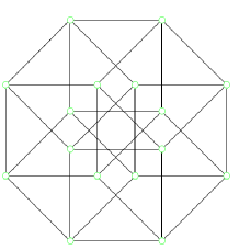
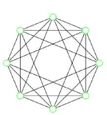
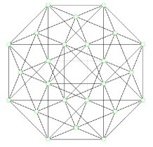
Figure 14: OctogonalCox24cell projection of the tesseract, the 16-cell and the 24-cellCoxBook .

The demitesseract belongs to the family of demihypercubes, also called half measure polytopes and denoted by $h\gamma_{n}$, which are constructed from hypercubes by deleting half of the vertices and forming new facets in place of the deleted vertices CoxIII (see Figure 15).

Figure 15: Projection of a demitesseract (in red) constructed on the vertices of a tesseract.

The demitesseract is the demihypercube in dimension $4$. As a polytope, the demitesseract is identical to the regular hexadecachoron.

Figure 16: A hexadecachoron (in red) whose vertices are the centers of the cells of a tesseract.

Whilst the hexadecachoron and the demitesseract are identical as polytopes, their associated symmetries are different. Indeed, the reflection group of the hexadecachoron is $B_{4}$ that is the same of the tesseract. The reflections of the demitesseract generates a subgroup of index $2$ of $B_{4}$ whose associated mirrors are

$$x_{1}=x_{2},\ x_{2}=x_{3},\ x_{3}=x_{4},\mbox{ and }x_{1}+x_{2}=0.$$ (57)

This group is generated by the transpositions $x_{1}\leftrightarrow x_{2}$, $x_{2}\leftrightarrow x_{3}$, and $x_{3}\leftrightarrow x_{4}$ together with an additional generator which transposes $x_{1}$ and $x_{2}$ while reversing the sign of both. So, clearly these reflections generate a group isomorphic to $D_{4}$. The normalized demitesseract has $8$ vertices, whose coordinates are $(1,1,1,1)$, $(1,1,-1,-1)$, $(1,-1,1,-1)$, $(-1,1,1,-1)$, $(1,-1,-1,1)$, $(-1,1,-1,1)$, $(-1,-1,1,1)$, and $(-1,-1,-1,-1)$, $24$ edges, $32$ triangular faces and $16$ tetrahedral cells.

Appendix B Discussion on the quartics $Q_{1}$, $Q_{2}$ and $Q_{3}$

First we focus the discussion on the number of zero roots of the quartic. We have to treat several cases.

B.1 The three quartics have at least a zero root

This implies that $L=M=0$ and this has been completely investigated in our previous paperHLT2 . The quartics are

$$Q_{1}=Q_{2}=Q_{3}=x^{4}-2Bx^{3}y+B^{2}x^{2}y^{2}+4D_{xy}xy^{3}.$$ (58)

If $D_{xy}=0$, the quartics have at least two zero roots and we obtain

$$Q_{1}=Q_{2}=Q_{3}=x^{2}(By-x)^{2}.$$ (59)

So the only special case occurs when $B=0$ and corresponds to the nilpotent forms. The classification of nilpotent forms is well-known and is due to Djokovic et al. CD ; DLS (see also the previous paper of the authors HLT2 for the geometrical interpretation). Note also that the case when $B\neq 0$ has been already algebraically and geometrically described HLT2 .
If $D_{xy}\neq 0$ then the discriminant is

$$\Delta=D_{xy}(27D_{xy}-B^{3}).$$ (60)

One has first to examine the case when the roots of each quartic are distinct. This corresponds to $\Delta\neq 0$ and has been investigated in our previous paperHLT2 (no other cases appear in the present discussion).
If the quartics have nonzero multiple roots then the forms belong to the variety defined by

$$27D_{xy}-B^{3}=0.$$ (61)

This variety have been also investigated in our previous paperHLT2 . Nevertheless the present discussion may refine the classification by regarding the other covariants of the quartics:

$$\begin{array}[]{rcl}T&=&1152(D_{xy}x^{6}+D_{xy}Bx^{5}y+10D_{xy}^{2}x^{3}y^{2}-5D_{xy}^{2}Bx^{2}y^{4}+B^{2}D_{xy}^{2}xy^{5}+2D_{xy}^{3}y^{6})\\ Hess&=&-12(B^{2}x^{4}-2(12D_{xy}+B^{3})x^{3}y+B(12D_{xy}+B^{3})x^{2}y^{2}+4B^{2}D_{xy}xy^{3}+12D_{xy}^{2}y^{4})\\ I_{2}&=&2BD_{xy}+\frac{1}{12}H^{4}\\ I_{3}&=&-(D_{xy}^{2}+\frac{1}{216}B^{6}+\frac{1}{6}B^{3}D_{xy}).\end{array}$$ (62)

Since $D_{xy}\neq 0$ the covariants $T$ and $Hess$ are clearly nonzero. According to Table 1 the only case to investigate is $I_{2}=I_{3}=0$. But this implies $B=D_{xy}=0$ and this case has already been dealt with. It follows that all the interesting cases have been already investigated in our previous article HLT2 .

B.2 Only one of the quartics has a zero roots

B.2.1 The quartic $Q_{1}$ has a zero root

In this case, one has $L=0$ and $M=-N$ (we will see that the other two cases are symmetrical). The quartics are

$$Q_{1}=x^{4}-2Bx^{3}y+(B^{2}+4M)x^{2}y^{2}+4(D_{xy}-BM)xy^{3},$$ (63)

$$Q_{2}=Q_{3}=x^{4}-2Bx^{3}y+(B^{2}-2M)x^{2}y^{2}-2(BM-2D_{xy})xy^{3}+M^{2}y^{4}.$$ (64)

The covariants reads

$$I_{2}=2B(D_{xy}-BM)+\frac{1}{12}(B^{2}+4M)^{2},$$ (65)

$$I_{3}=-(D_{xy}-BM)^{2}-\frac{1}{216}(B^{2}+4M)^{3}-\frac{1}{6}B(B^{2}+4M)(D_{xy}-BM),$$ (66)

$$\begin{array}[]{rcl}Hess(Q_{1})&=&-12\,({{\it B}}^{2}-8\,{\it M}){x}^{4}+24\,({{\it B}}^{3}-8\,{\it B}\,{\it M}+12\,{\it D_{xy}}){x}^{3}y-12\,(12\,{\it B}\,{\it D_{xy}}-4\,{{\it B}}^{2}{\it M}\\ &&+{{\it B}}^{4}+16\,{{\it M}}^{2})x^{2}{y}^{2}+48\,({{\it B}}^{2}+4\,{\it M})(-{\it D_{xy}}+{\it B}\,{\it M})x{y}^{3}-144\,(-{\it D_{xy}}+{\it B}\,{\it M})^{2}{y}^{4},\end{array}$$ (67)

$$\begin{array}[]{rcl}Hess(Q_{2})&=&-12\,\left({{\it B}}^{2}+4\,{\it M}\right){x}^{4}+24\,({{\it B}}^{3}-8\,{\it B}\,{\it M}+12\,{\it D_{xy}}){x}^{3}y-12\,(-10\,{{\it B}}^{2}{\it M}+12\,{\it B}\,{\it D_{xy}}\\ &&+{{\it B}}^{4}-8\,{{\it M}}^{2})x^{2}{y}^{2}+24\,({{\it B}}^{3}{\it M}-2\,{{\it B}}^{2}{\it D_{xy}}-8\,{\it B}\,{{\it M}}^{2}+4\,{\it M}\,{\it D_{xy}})x{y}^{3}\\ &&-12\,({{\it B}}^{2}{{\it M}}^{2}+4\,{{\it M}}^{3}-12\,{\it D_{xy}}\,{\it B}\,{\it M}+12\,{{\it D_{xy}}}^{2}){y}^{4},\end{array}$$ (68)

$$\begin{array}[]{rcl}T(Q_{1})&=&-1152(\,{\it D_{xy}}\,{x}^{6}-({\it B}\,{\it D_{xy}}+4\,{{\it M}}^{2}){x}^{5}y+10\,{\it M}\,(-{\it D_{xy}}+{\it B}\,{\it M})x^{4}{y}^{2}\\ &&-10\,(-{\it D_{xy}}+{\it B}\,{\it M})^{2}{x}^{3}{y}^{3}+5\,{\it B}\,(-{\it D_{xy}}+{\it B}\,{\it M})^{2}x^{2}{y}^{4}\\ &&-\,({{\it B}}^{2}+4\,{\it M})(-{\it D_{xy}}+{\it B}\,{\it M})^{2}x{y}^{5}+2\,(-{\it D_{xy}}+{\it B}\,{\it M})^{3}{y}^{6}),\end{array}$$ (69)

and

$$\begin{array}[]{rcl}T(Q_{2})&=&-1152\,({\it D_{xy}}-{\it B}\,{\it M})({x}^{6}-{\it B}\,{x}^{5}y+5\,{\it M}\,x^{4}{y}^{2}-10\,{\it D_{xy}}\,x^{3}{y}^{3}\\ &&+5(\,{\it B}\,{\it D_{xy}}-\,{{\it M}}^{2})x^{2}{y}^{4}-({{\it B}}^{2}{\it D_{xy}}-{\it B}\,{{\it M}}^{2}-2\,{\it M}\,{\it D_{xy}})x{y}^{5}\\ &&+({\it D_{xy}}\,{\it B}\,{\it M}-{{\it M}}^{3}+2\,{{\it D_{xy}}}^{2}){y}^{6}).\end{array}$$ (70)

According to Table 1, we have to investigate several cases.
$\bullet$ The quartic $Q_{1}$ has a double zero root
This case is identified by the equation $D_{xy}=BM$ and implies automatically $\Delta=0$. The quartics are

$$Q_{1}=x^{4}-2Bx^{3}y+(B^{2}+4M)x^{2}y^{2},$$ (71)

$$Q_{2}=Q_{3}=(-x^{2}+Bxy+y^{2})^{2}.$$ (72)

The covariants simplify as

$$I_{2}=\frac{1}{2}(B^{2}+4M)^{2},$$ (73)

$$I_{3}=\frac{1}{216}(B^{2}+4M)^{3},$$ (74)

$$T(Q_{1})=-1152(BMx^{6}-M(B^{2}+4M)x^{5}y),$$ (75)

$$Hess(Q_{1})=-12(B^{2}-8M)x^{4}+24(B^{2}+4M)Bx^{3}y-12(B^{2}+4M)^{2}x^{2}y^{2},$$ (76)

$$Hess(Q_{2})=Hess(Q_{3})=-12(B^{2}+4M)(Bxy+My^{2}-x^{2})^{2}.$$ (77)

Since $Q_{2}$ has two double roots, one has $T(Q_{2})=0$. It remains to examine the following cases

1. If $Q_{1}$ has two simple distinct nonzero roots then $B^{2}+4M\neq 0$. It follows that $I_{2},I_{3}\neq 0$ and $Q_{2}$ has no triple root. The only remaining case to consider is the case when $Q_{2}$ has a quadruple root. But this implies $B^{2}+4M=0$ and so it is not possible.

2. If $Q_{1}$ has a nonzero double root then $T(Q_{1})=0$ and this implies $M=D_{xy}=0$. This configuration cannot occur since it implies that $Q_{2}$ has a zero root.

3. If $Q_{1}$ has a triple zero root then $B^{2}+4M=0$ and $Hess(Q_{2})=0$. Hence, $Q_{2}$ has a quadruple root.

4. If $Q_{1}$ has a quadruple zero root then $M=0$. So this configuration is not possible.

In conclusion, when $L=0$ and $M\neq 0$, we have only to investigate the variety given by $B^{2}+4M=0$.

$\bullet$ $Q_{1}$ has a nonzero double root and two simple roots
Since the zero roots of $Q_{1}$ is not double, one has $D_{xy}\neq BM$ and then $T(Q_{1}),T(Q_{2})\neq 0$. This prove that $Q_{2}$ has exactly one double root.
$\bullet$ $Q_{1}$ has a triple nonzero root
We have $D_{xy}\neq BM$ and $I_{2}=I_{3}=0$. The equation $I_{2}=I_{3}=0$ admits two solutions: $\{M=-\frac{1}{4}B^{2},D_{xy}=-\frac{1}{4}B^{3}\}$ and $\{M=\frac{1}{12}B^{2},D_{xy}=\frac{1}{108}B^{3}\}$. The first solution implies $D_{xy}=BM$, so it must be excluded. From the second solution, we deduce

$$T(Q_{1})=-\frac{32}{2187}B^{3}(2By-3x)^{6},$$ (78)

$$T(Q_{2})=\frac{4}{2187}B^{3}(By-6x)^{6},Hess(Q_{1})=-\frac{4}{81}B^{2}(2By-3x)^{4},$$ (79)

$$Hess(Q_{2})=-\frac{1}{81}B^{2}(By-6x)^{4}.$$ (80)

The only special case is $B=0$ and that the form is nilpotent.
$\bullet$ $Q_{1}$ has only simple roots
In this case $Q_{2}$ has also only simple roots. This case corresponds to

$$\Delta=(B^{3}D_{xy}-B^{2}M^{2}-18D_{xy}BM+16M^{3}+27D_{xy})(BM-D_{xy})^{2}\neq 0.$$ (81)

B.2.2 $Q_{2}$ has a zero root

In this case, one has $M=0$ and $L=-N$. The quartics are

$$Q_{2}=x^{4}-2Bx^{3}y+(B^{2}-4L)x^{2}y^{2}+4D_{xy}xy^{3},$$ (82)

$$Q_{1}=Q_{3}=x^{4}-2Bx^{3}y+(B^{2}+2L)x^{2}y^{2}-2(BL-2D_{xy})xy^{3}+L^{2}y^{4}.$$ (83)

The covariants read

$$I_{2}=3\left(\frac{1}{6}B^{2}-\frac{2}{3}L\right)^{2}+2BD_{xy},$$ (84)

$$I_{3}=-D_{xy}^{2}-\left(\frac{1}{6}B^{2}-\frac{2}{3}L\right)^{3}-B\left(\frac{1}{6}B^{2}-\frac{2}{3}L\right)D_{xy},$$ (85)

$$\begin{array}[]{rcl}Hess(Q_{2})&=&-12\,\left({{\it B}}^{2}+8\,{\it L}\right){x}^{4}+24\,({{\it B}}^{3}-4\,{\it B}\,{\it L}+12\,{\it D_{xy}}){x}^{3}y-12\,(-8\,{{\it B}}^{2}{\it L}+12\,{\it B}\,{\it D_{xy}}\\ &&+{{\it B}}^{4}+16\,{{\it L}}^{2})x^{2}{y}^{2}-48(B^{2}-4L)x{y}^{3}-144\,{{\it D_{xy}}}^{2}){y}^{4},\end{array}$$ (86)

$$\begin{array}[]{rcl}Hess(Q_{1})&=&-12\,\left({{\it B}}^{2}-4\,{\it L}\right){x}^{4}+24\,({{\it B}}^{3}-4\,{\it B}\,{\it L}+12\,{\it D_{xy}}){x}^{3}y-12\,(-2\,{{\it B}}^{2}{\it M}+12\,{\it B}\,{\it D_{xy}}\\ &&+{{\it B}}^{4}-8\,{{\it L}}^{2})x^{2}{y}^{2}-24\,(-{{\it B}}^{3}{\it L}+2\,{{\it B}}^{2}{\it D_{xy}}+4\,{\it B}\,{{\it L}}^{2}+4\,{\it L}\,{\it D_{xy}})x{y}^{3}\\ &&-12\,({{\it B}}^{2}{{\it L}}^{2}-4\,{{\it L}}^{3}-12\,{\it D_{xy}}\,{\it B}\,{\it L}+12\,{{\it D_{xy}}}^{2}){y}^{4},\end{array}$$ (87)

$$\begin{array}[]{rcl}T(Q_{2})&=&-1152(\,{\it D_{xy}}-BL)\,{x}^{6}-({\it B}\,{\it D_{xy}}+4\,{{\it L}}^{2}-B^{2}L){x}^{5}y+10\,{\it L}{\it D_{xy}}x^{4}{y}^{2}\\ &&-10\,D_{xy}^{2}{x}^{3}{y}^{3}+5\,{\it B}D_{xy}^{2}x^{2}{y}^{4}-\,({{\it B}}^{2}-4\,{\it L})D_{xy}^{2}x{y}^{5}-2\,D_{xy}^{3}{y}^{6}),\end{array}$$ (88)

and

$$\begin{array}[]{rcl}T(Q_{1})&=&-1152\,{\it D_{xy}}({x}^{6}-{\it B}\,{x}^{5}y-5\,{\it L}\,x^{4}{y}^{2}-10\,({\it D_{xy}}-BL)\,x^{3}{y}^{3}\\ &&+5(\,{\it B}\,{\it D_{xy}}-B^{2}L-\,{{\it L}}^{2})x^{2}{y}^{4}-({{\it B}}^{2}{\it D_{xy}}-B^{3}L+2LD_{xy}-3BL^{2})x{y}^{5}\\ &&-(B^{2}L^{2}-L^{3}+2D_{xy}^{2}-3BLD_{xy}){y}^{6}).\end{array}$$ (89)

Hence, the reasoning is very similar to the case $L=0$. Let us summarize it below.
According to table 1, we have to investigate several cases.
$\bullet$ The quartic $Q_{2}$ has a double zero root
The case is identified by the equation $D_{xy}=0$ and implies $\Delta=0$, $Q_{1}=Q_{3}=(x^{2}-Bxy+L^{2}y^{2})^{2}$, $Q_{2}=x^{2}(x^{2}-2Bxy+(B^{2}-4L)y^{2})$, $I_{2}=\frac{1}{12}(B^{2}-4L)^{2}$ and $I_{3}=-\frac{1}{216}(B^{2}-4L)^{3}$. Hence, when $L\neq 0$ and $M=0$, we have only to investigate the variety given by $B^{2}-4L=0$. This corresponds the case when $Q_{1}$ has a quadruple root and $Q_{2}$ has a triple zero root.
$\bullet$ $Q_{2}$ has a nonzero double root and two simple roots
In this case, $D_{xy}\neq 0$ and so $T(Q_{1}),T(Q_{2})\neq 0$. So $Q_{1}$ has exactly one double root.
$\bullet$ $Q_{2}$ has a triple nonzero root
The only solution of $I_{2}=I_{3}=M=0$ satisfying $D_{xy}\neq 0$ is $D_{xy}=-\frac{2}{27}B^{3}$ and $L=-\frac{1}{12}B^{2}$. The only special case is $B=0$ and implies the nilpotence of the form.
$\bullet$ $Q_{2}$ has only simple roots
In this case $Q_{1}$ has also four distinct roots. Furthermore, the hyperdeterminant factorizes as

$$\Delta=D_{xy}^{2}(36BLD_{xy}+B^{4}L-B^{3}D_{xy}-27D_{xy}^{2}+16L^{3}-8B^{2}L^{2}).$$

B.2.3 $Q_{3}$ has a zero root

In this case, one has $N=0$ and $L=-M$. The quartics are

$$Q_{3}=x^{4}-2Bx^{3}y+(B^{2}-4M)x^{2}y^{2}+4D_{xy}xy^{3},$$ (90)

$$Q_{1}=Q_{2}=x^{4}-2Bx^{3}y+(B^{2}+2M)x^{2}y^{2}-2(BM-2D_{xy})xy^{3}+M^{2}y^{4}.$$ (91)

So it is deduced by substituting $L\leftrightarrow M$ and $Q_{2}\leftrightarrow Q_{3}$ in the previous discussion ($M=0$).

B.3 The quartics have no zero root

We have to investigate three cases.

B.3.1 $Q_{1}$ has four simple roots

This means that $\Delta\neq 0$ and then $Q_{2}$ and $Q_{3}$ have both four simple roots.

B.3.2 $T(Q_{1})=0$

The equation $T(Q_{1})=0$ a has two solutions: $M=D_{xy}=0$ and $N=D_{xy}=0$. In this two cases, one of the quartic has a zero root. In the same way, if $T(Q_{2})=0$ or $T(Q_{3})=0$ then one of the quartic has a zero root.

B.3.3 $T(Q_{1}),T(Q_{2}),T(Q_{3})\neq 0$

Since $Hess=0$ implies $T=0$ (if a form has a quadruple root then it has two double roots which are equal), one has two cases to consider:

1. $I_{2},I_{3}\neq 0$,

2. $I_{2}=I_{3}=0$.

Appendix C Symmetries of the Verstraete forms

C.1 Permutations of the qubits

Versraete et al.VDMV gave nine inequivalent normal forms for the four qubic forms. These forms were defined up to a permutation of qubits. One of these forms $G_{abcd}$ has $4$ parameters and the set of all the $G_{abcd}$ defines a $4$-dimension subspace of the ambient space. The five other forms, $L_{abc_{2}},L_{a_{2}b_{2}},L_{ab_{3}},L_{a_{4}}$ and $L_{a_{2}0_{3\oplus\overline{1}}}$ have one to three parameters and define five affine subspaces. The remaining three forms, $L_{0_{5\oplus\overline{3}}},L_{0_{7\oplus\overline{1}}}$ and $L_{0_{3\oplus\overline{1}}0_{3\oplus\overline{1}}}$ are nilpotent. For a given form $\varphi$, we will denote by $\varphi^{\sigma}$ the form obtained by applying the permutation $\sigma$ on the qubits. For the more generic form $G_{abcd}$, we obtain $5$ other non equivalent forms $G_{abcd}^{1423}$, $G_{abcd}^{1324}$, $G_{abcd}^{1243}$, $G_{abcd}^{1324}$ and $G_{abcd}^{1432}$. Each of them is equivalent to a $G_{a^{\prime}b^{\prime}c^{\prime}d^{\prime}}$ for one of the following specializations (which are involutions):

• $(a,b,-c,d)$,

• $(\frac{a+b-c+d}{2},\frac{a+b+c-d}{2},\frac{-a+b+c+d}{2},\frac{a-b+c+d}{2})$,

• $(\frac{a+b-c+d}{2},\frac{a+b+c-d}{2},\frac{a-b-c-d}{2},\frac{-a+b-c-d}{2})$,

• $(\frac{a+b+c+d}{2},\frac{a+b-c-d}{2},\frac{a-b-c+d}{2},\frac{-a+b-c+d}{2})$,

• and $(\frac{a+b+c+d}{2},\frac{a+b-c-d}{2},\frac{a-b+c-d}{2},\frac{a-b-c+d}{2})$.

The permutations of $L_{abc_{2}}$ split into $6$ families with representatives $L_{abc_{2}}$,$L^{1342}_{abc_{2}}$,$L_{abc_{2}}^{2431}$,$L_{abc_{2}}^{1432}$,$L_{abc_{2}}^{2341}$,and $L_{abc_{2}}^{2143}$.Furthermore, we have

$$L^{1324}_{\left(\frac{a+b}{2}+c,\frac{a+b}{2}-c,\frac{a-b}{2}\right)}\sim L^{1243}_{abcc},\ L^{2431}_{\left(\frac{a+b}{2}+c,\frac{a+b}{2}-c,\frac{a-b}{2}\right)}\sim L^{2134}_{abcc},$$

$$L^{1432}_{\left(\frac{a+b}{2}+c,\frac{a+b}{2}-c,\frac{a-b}{2}\right)}\sim L^{1423}_{abcc},\ L^{1234}_{\left(\frac{a+b}{2}+c,\frac{a+b}{2}-c,\frac{a-b}{2}\right)}\sim L^{1324}_{abcc},$$

$$L^{2341}_{\left(\frac{a+b}{2}+c,\frac{a+b}{2}-c,\frac{a-b}{2}\right)}\sim L^{2314}_{abcc},\ L^{2143}_{\left(\frac{a+b}{2}+c,\frac{a+b}{2}-c,\frac{a-b}{2}\right)}\sim L^{2413}_{abcc}.$$

There are also $6$ different families of permutations of $L_{ab_{3}}$ whose representatives are $L^{\sigma}_{ab_{3}}$ for $\sigma\in\{1234,1423,3421,1342,3412\}$. The permutations of $L_{a_{2}b_{2}}$ generate $12$ non equivalent families $L^{\sigma}_{a_{2}b_{2}}$ for $\sigma\in\{1234,2314,2413,1324,1243,2134,2431,2143,3241,3124,3214\}$. The permutations $L_{a_{4}}^{\sigma}$ for $\sigma\in{\mathfrak{S}}_{4}$ are pairwise nonequivalent. Finally, the permutations of $L_{a_{2}0_{3\oplus\overline{1}}}$ give $4$ nonequivalent families $L_{a_{2}0_{3\oplus\overline{1}}}^{1234}$, $L_{a_{2}0_{3\oplus\overline{1}}}^{2134}$, $L_{a_{2}0_{3\oplus\overline{1}}}^{2341}$, and $L_{a_{2}0_{3\oplus\overline{1}}}^{2314}$.

If we send each parameter to zero, the permutations of the Verstraete forms specialize to nilpotent orbits. To each form corresponds one of the strata defined in our previous paper HLT2 see Table 8.

Forms	Strata
$G_{abcd}$	$Gr_{0}$
$L_{abc_{2}}$	$Gr_{1}$
$L_{a_{2}b_{2}}$	$Gr_{2}$
$L_{a_{2}0_{3\oplus\overline{1}}}$	$Gr_{3}$
$L_{0_{3\oplus\overline{1}}0_{3\oplus\overline{1}}}$	$Gr_{4}$
$L_{ab_{3}}$	$Gr_{5}$
$L_{a_{4}}$	$Gr_{6}$
$L_{0_{5\oplus\overline{3}}}$	$Gr_{7}$
$L_{0_{7\oplus\overline{1}}}$	$Gr_{8}$

Table 8: Correspondence between Verstraete forms and nilpotent strata

C.2 Quadrics again

In a general setting, permuting the qubits in a form induces a permutations on the quadrics $Q_{1},Q_{2},Q_{3}$. Let us denote $\mathcal{Q}(\varphi)=\{Q_{1}(\varphi),Q_{2}(\varphi),Q_{3}(\varphi)\}$. We notice also that any of the quadrics in the Verstraete forms can be written as $Q_{1}(G_{abcd})$ for some specialization of the parameters $a$, $b$ and $c$. Indeed we have

$$\mathcal{Q}(G_{abcd})=\left\{Q_{1}\left(G_{abcd}\right),Q_{1}\left(G_{\frac{a+c-d-b}{2}\frac{a+d-b-c}{2}\frac{a+b-c-d}{2}\frac{a+b+c+d}{2}}\right){}Q_{1}\left(G_{\frac{a+b+c-d}{2}\frac{a+b-c+d}{2}\frac{a-b+c+d}{2}\frac{-a+b+c+d}{2}}\right)\right\}.$$

The remaining values are summarized in Table 9.

$$\begin{array}[]{|c|c|c|c|c|c|c|}\hline\cr\mbox{Forms}&\mathcal{Q}(G_{abcd})&\mathcal{Q}(L_{abc_{2}})&\mathcal{Q}(L_{ab_{3}})&\mathcal{Q}(L_{a_{2}b_{2}})&\mathcal{Q}(L_{a_{4}})&\mathcal{Q}(L_{a_{2}0_{3\oplus\overline{1}}})\\ \hline\cr G_{abcd}&\mathcal{Q}(G_{abcd})&&&&&\\ L_{abc_{2}}&\mathcal{Q}\left(G_{abcc}\right)&&&&&\\ L_{ab_{3}}&\mathcal{Q}\left(G_{aaab}\right)&\mathcal{Q}(L_{aba})&&&&\\ L_{a_{2}b_{2}}&\mathcal{Q}\left(G_{aabb}\right)&\mathcal{Q}(L_{aab})&&&&\\ L_{a_{4}}&\mathcal{Q}\left(G_{aaaa}\right)&\mathcal{Q}(L_{aaa})&\mathcal{Q}(L_{aa_{3}})&&&\\ L_{a_{2}0_{3\oplus\overline{1}}}&\mathcal{Q}\left(G_{aa00}\right)&\mathcal{Q}(L_{aa0})&\mathcal{Q}(L_{a_{2}0_{2}})&&&\\ \hline\cr L_{0_{5\oplus\overline{3}}}&\mathcal{Q}\left(G_{0000}\right)&\mathcal{Q}(L_{000})&\mathcal{Q}(L_{0_{2}0_{2}})&\mathcal{Q}(L_{00_{3}})&\mathcal{Q}(L_{0_{4}})&\mathcal{Q}(L_{0_{2}0_{3\oplus\overline{1}}})\\ L_{0_{7\oplus\overline{1}}}&\mathcal{Q}\left(G_{0000}\right)&\mathcal{Q}(L_{000})&\mathcal{Q}(L_{0_{2}0_{2}})&\mathcal{Q}(L_{00_{3}})&\mathcal{Q}(L_{0_{4}})&\mathcal{Q}(L_{0_{2}0_{3\oplus\overline{1}}})\\ L_{0_{3\oplus\overline{1}}0_{3\oplus\overline{1}}}&\mathcal{Q}\left(G_{0000}\right)&\mathcal{Q}(L_{000})&\mathcal{Q}(L_{0_{2}0_{2}})&\mathcal{Q}(L_{00_{3}})&\mathcal{Q}(L_{0_{4}})&\mathcal{Q}(L_{0_{2}0_{3\oplus\overline{1}}})\\ \hline\cr\end{array}$$

Table 9: Values of $\mathcal{Q}$ for Verstraete forms

References

- (1) Arnol’d V., “Normal forms for functions near degenerate critical points, the Weyl groups of A k, D k, E k and Lagrangian singularities.” Functional Analysis and its applications 6.4 (1972): 254-272.
- (2) Borsten L., Dahanayake D., Duff M. J., Marrani A. and Rubens W., “Four-Qubit Entanglement Classification from String Theory”, Phys. Rev. Lett. 105, 100507 (2010).
- (3) Borsten L., Duff M. J., and Levay P., “The black-hole/qubit correspondence: an up-to-date review.”, arXiv preprint arXiv:1206.3166 (2012).
- (4) Briand E., Luque J.-G., Thibon J.-Y., “A complete set of covariants of the four-qubit system” Journal of Physics A: mathematical and general. 36.38 (2003): 9915.
- (5) Cao Y., and Wang. A. M. "Discussion of the entanglement classification of a 4-qubit pure state." The European Physical Journal D 44, no. 1 (2007): 159-166.
- (6) Chen L. Doković D., Grassl M and Zeng B. "Four-qubit pure states as fermionic states." Physical Review A 88, no. 5 (2013): 052309.
- (7) Chterental O. and Djokovic D., “Normal forms and tensor ranks of pure states of four-qubit”, arXiv preprint quant-ph/0612184 (2006).
- (8) Coxeter H.S.M., Regular polytopes, Dover publications, inc. New York (1973).
- (9) Coxeter H.S.M., “Two aspects of the regular -cell in four dimensions”, in Kaleidoscopes, selected writing of H.S. Coxeter, Wiley-Interscience publication (1995).
- (10) Coxeter H.S.M., “ Regular and semiregular polytopes.III”, in Kaleidoscopes, selected writing of H.S. Coxeter, Wiley-Interscience publication (1995).
- (11) Coxeter H.S.M., Complex regular polytopes. Cambridge University Press; 2 edition (April 26, 1991)
- (12) Dimca, A. (1986). “Milnor numbers and multiplicities of dual varieties”. Revue Roumaine de Mathématiques Pures et Appliquées, 31(6), 535-538.
- (13) Djokovic D., Lemire N. and Sekiguchi J., “The closure ordering of adjoint nilpotent orbits in ”, Tohoku Mathematical Journal 53.3 (2001): 395-442.
- (14) Eltschka C., and Siewert. "Quantifying entanglement resources." Journal of Physics A: Mathematical and Theoretical 47, no. 42 (2014): 424005.
- (15) W. Fulton, J. Harris, Representation Theory, Graduate Text in Mathematics, Springer 1991.
- (16) Gour G. and Wallach N., “On symmetric SL-invariant polynomials in four-qubit.” In Symmetry: Representation Theory and Its Applications, pp. 259-267. Springer New York, 2014.
- (17) Gelfand I.M., Kapranov M.M., Zelevinsky A.V., “Hyperdeterminants”, Advances in Mathematics 96, vol 2 (1992).
- (18) I.M Gelfand M.M Kapranov A.V. Zelevinsky, Discriminants, Resultants and Multidimensional Determinants, Birkhäuser 1994.
- (19) Grassl, M., Beth, T., and Pellizzari, T. (1997). “Codes for the quantum erasure channel”. Physical Review A, 56(1), 33.
- (20) Gühne, O., Jungnitsch, B., Moroder, T. and Weinstein, Y. S. (2011). “Multiparticle entanglement in graph-diagonal states: Necessary and sufficient conditions for four qubits”. Physical Review A, 84(5), 052319.
- (21) J. Harris, Algebraic Geometry: a first course, Graduate Texts in Mathematics 133 Springer 1992.
- (22) Heydari H., “Geometrical Structure of Entangled States and the Secant Variety”, Quantum Information Processing 7 (1), 3-32 (2008).
- (23) Holweck, F. and Lévay, P., 2016. “Classification of multipartite systems featuring only and genuine entangled states”. Journal of Physics A: Mathematical and Theoretical, 49(8), (2016) p.085201.
- (24) Holweck F., Luque J.-G., and Planat M. "Singularity of type D4 arising from four-qubit systems." Journal of Physics A: Mathematical and Theoretical 47.13 (2014): 135301.
- (25) Holweck F., Luque J.-G., Thibon J.-Y., “Geometric descriptions of entangled states by auxiliary varieties”, Journal of Mathematical Physics 53, 102203 (2012).
- (26) Holweck F., Luque J.-G., Thibon J.-Y., “Entanglement of four-qubit systems: a geometric atlas with polynomial compass I (the finite world)”. a completer.
- (27) Horodecki R., Horodecki P., Horodecki M., Horodecki K., “Quantum entanglement“, Reviews of Modern Physics, 81(2), 865 (2009).
- (28) T. Ivey, J.M. Landsberg, Cartan for beginners: Differential Geometry via Moving Frames and Exterior Differential Systems, Graduate Studies in Mathematics 61 2003.
- (29) Lamata L., León J., Salgado D. and Solano E., “Inductive entanglement classification of four-qubit under stochastic local operations and classical communication”, Phys. Rev. A. 72, 022318 (2007).
- (30) Landsberg J. M., Tensors: Geometry and applications, Vol. 128. Amer Mathematical Society, 2011.
- (31) Lévay, P., "On the geometry of four-qubit invariants." Journal of Physics A: Mathematical and General 39.30 (2006): 9533.
- (32) Lévay P., “STU black holes as four-qubit systems”, Pys. Rev. D 82, 026003 (2010).
- (33) Lévay P. and Holweck F., "Embedding qubits into fermionic Fock space: Peculiarities of the four-qubit case." Physical Review D 91.12 (2015): 125029.
- (34) Li D., Li X., and Huang H., "SLOCC classification for nine families of four-qubits." arXiv preprint arXiv:0712.1876 (2007).
- (35) Lin S. and Sturmfels B. "Polynomial relations among principal minors of a -matrix." Journal of Algebra 322, no. 11 (2009): 4121-4131.
- (36) Luque J.-G. and Thibon J.-Y, “The polynomial invariants of four-qubit”, Phys. Rev. A 67, 042303 (2003).
- (37) Luque, J.-G., and Thibon J.-Y, “Algebraic invariants of five qubits” Journal of physics A: mathematical and general 39, no. 2 (2005): 371.
- (38) Miyake A., “Classification of multipartite entangled states by multidimensional determinants”, Phys. Rev. A 67, 012108 (2003).
- (39) Olver P., Classical Invariant Theory, Cambridge University Press, Cambridge UK, 1999.
- (40) Parusiński, A. “Multiplicity of the dual variety”. Bulletin of the London Mathematical Society, 23(5), 429-436. (1991).
- (41) Popov V., Vinberg E., "Invariant theory." Algebraic geometry IV. Springer Berlin Heidelberg, 1994. 123-278.
- (42) Tevelev E. A., “Projectively Dual Varieties”, Journal of Mathematical Sciences 117 (6), 4585-4732 (2003).
- (43) Verstraete F., Dehaene F., De Moor B. and Verschelde H., “Four qubits can be entangled in nine different ways”, Phys. Rev.. A 65, 052112 (2002).
- (44) Weyman J. and Zelevinsky A., “Singularities of Hyperdeterminants”, Annales de l’Institut Fourier 46, 591-644 (1996).
- (45) F. Zak, Tangents and Secants of Algebraic Varieties, AMS Translations of mathematical monographs 127 1993.
- (46) F. Zak, Determinants of projective varieties and their degrees, Algebraic Transformation Groups and Algebraic Varieties, Encyclopaedia of Mathematical Sciences, vol. 132, Subseries Invariant Theory and Algebraic Transformation Groups, vol. III, Springer-Verlag, Berlin-Heidelberg-New York, 2004.